Abstract
An objective classification scheme by Jenkinson and Collison is applied to the period 1961–2010 to statistically model the temperatures over Serbia. The originally identified 26 weather types (WTs) are reorganised into 10 basic types. This discussion includes the synoptic characteristics, frequency and trends of the 10 WTs as well as the trends of seasonal mean, maximum and minimum temperatures in Serbia. In this area, the anticyclonic weather type is predominant throughout the year, and its negative trend is significant in summer and autumn. The relationship between air temperature and atmospheric circulation types is investigated by analysing the mean and anomalies of mean, maximum and minimum temperatures for each individual atmospheric circulation type and by stepwise regression. The multiple regression models developed for six stations using circulation WTs as predictors showed the best performance in modelling winter mean temperatures for Zlatibor and Loznica compared to the other stations, while the models for other seasons proved to be inadequate.
1. Introduction
Atmospheric circulation is of fundamental importance for determining climatic and meteorological conditions. Therefore, the relationships between large-scale circulation and local meteorological conditions, including the occurrence of extreme phenomena and events, are frequently studied [1]. Classifications of atmospheric circulation are usually operationalized.
The Lamb weather types, developed by climatologist Hubert Lamb in the mid-20th century, are a classification system used to categorize and describe the various atmospheric circulation patterns that influence European weather [2]. The original development of this manual (subjective) scheme was intended for the British Isles [3,4]. In 1977, Jenkinson and Collison introduced an objective classification of WT using mean sea level pressure (MSLP) data on a relatively coarse grid, intended to fulfil the same purpose as the Lamb classification [5]. The application of this classification to regions outside the British Isles requires an adaptation of the grid point arrangement to the particular area of interest. Over the last 30 years, interest in automatic classification methods has increased. In addition to objective systems based on existing catalogues of circulation types, there are also systems that use statistical grouping methods [6,7,8]. In recent years, new automated methods for classifying circulation types using deep learning have been introduced [9].
Air temperature is one of the most important climatological variables, as it directly influences energy flows in the atmosphere, evaporation, the moisture balance of the soil and the occurrence of extreme weather events. Daily maximum and minimum temperatures are of particular importance as they enable the detection of temperature extremes and the monitoring of climate trends [10]. Their analysis plays a key role in understanding climate change at both local and global scales. Various authors in the field of synoptic climatology have documented how daily circulation patterns influence temperatures in different parts of the world. For example, there is a close relationship between extreme temperatures and changes in the frequency of Hess–Brezowsky circulation patterns over Central Europe [11,12]. In addition, the relationship between surface temperature and the large-scale circulation over the eastern Mediterranean, including Greece, is the subject of extensive research [13,14,15,16,17]. Peña-Angulo et al. [18] and Pérez and García [19] have identified weather types and associated temperatures in the Iberian Peninsula. Other authors have investigated classifications of daily circulation in southern South America and their relationships to the austral winter surface temperature in Argentina [20,21,22,23].
Several articles have discussed air temperatures over Serbia and the effects of atmospheric circulation on temperature in extreme cases. For example, Unkašević and Tošić [24] analysed the circulation conditions that led to extreme temperatures and heat waves in Serbia in the summer of 2007. In addition, the relationship between the large-scale circulation and the temperature in Serbia was analysed using teleconnection indices [25,26]. In their study, Tošić et al. [27] analysed extreme temperature events and possible connections between these events and the corresponding synoptic circulation patterns.
The aim of this study is to evaluate the ability of the method to describe the atmospheric circulation over the observed area, as well as to improve the understanding of the relationship between atmospheric circulation and air temperature in Serbia. This is approached in a novel way by using the weather types introduced by [28,29], which were analysed for the first time in these studies. The paper is organised as follows: Section 2 describes the data and methods used to achieve the objectives of the study; Section 3 presents the results; Section 4 provides a discussion of these results; and Section 5 provides brief conclusions.
2. Materials and Methods
2.1. Temperature in Serbia
The focus of this work is on Serbia, which is located in the central part of the Balkan Peninsula and partly in the Pannonian Basin in Central Europe (Figure 1). The country has a temperate continental climate with cold winters and hot summers, with varying degrees of local characteristics. The highest temperatures occur in July or August, while the lowest temperatures occur in December or January [30]. The spatial distribution of climate parameters is related to the geographical location, topography and local factors resulting from the combination of factors such as relief, distribution of atmospheric pressure in the large region, exposure of the terrain, presence of river systems, vegetation, urbanisation, etc. According to the Köppen climate classification, the predominant climate zone is Cfwbx″, while the hilly and mountainous parts are Dfwbx″ [31].
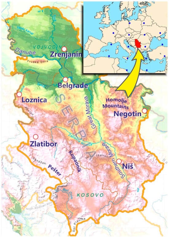
Figure 1.
Map of Serbia and stations used (list of stations with their abbreviations, latitudes, longitudes and altitudes) and grid points (blue dots) used to compute the vorticity and flow indices.
The daily mean, maximum and minimum temperatures (T, and , respectively) from 1961 to 2010 at six stations in Serbia (Figure 1) were provided by the Hydrometeorological Service of the Republic of Serbia. The stations were selected to represent the diversity and complexity of the Serbian terrain. A list of stations with their location and altitude is presented in Table 1. Only stations with complete data sets were included in the analysis. The Serbian Meteorological Service carried out both a technical and a professional validation of the measurements. The quality of the air temperature data was assessed using two quality control methods: (1) cases where the daily minimum temperature () exceeded the daily maximum temperature () and (2) values where the daily temperature was not between and and observations that deviated by ±4 standard deviations from T, , or , were flagged as potential outliers. No such anomalies were detected. The time series were then subjected to a quality control and homogeneity check according to the methodology described in [32]. All temperature series showed homogeneity.

Table 1.
Abbreviation of meteorological stations with their longitude, latitude and altitude (m).
2.2. Circulation Types
The classification according to Jenkinson and Collison is based on three main variables, which are derived exclusively from the mean air pressure at sea level. These variables are the wind direction (azimuth degree) (D), the wind speed (F) and the vorticity (Z) [28,33]. To determine the daily WTs, a certain resolution is used, with a set of 16 points centred over the designated area of interest. Once the atmospheric pressure is determined at 16 points, the three variables mentioned above are calculated using analytical expressions. Finally, 26 distinct circulation types are defined according to a set of rules [28,34]. Taking into account the set of rules, a total of 26 WTs are defined: 10 pure types (NE, E, SE, S, SW, W, NW, N, C and A) and 16 hybrid types (eight for each C or A hybrid). The eight pure types that are assigned to a specific wind direction are referred to as directional types.
In this work, the objective Jenkinson and Collison method of large-scale circulation patterns was applied to the atmospheric flow over Serbia. The geographical distribution for the 16-point grid with a resolution of latitude and longitude is shown in Figure 1. The selected location (32.5 to 52.5° N and 5 to 35° E) and a resolution of 5° latitude × 10° longitude were chosen because they best capture the characteristics of WTs over Serbia [28]. In order to develop a practical yet reliable statistical analysis scheme, the 26 circulation types were regrouped into ten basic types. The reduction was achieved by eliminating hybrid types. When encountering a hybrid type, 0.5 was incrementally added to the frequency series of cyclonic (C) or anticyclonic (A) types, and an additional 0.5 to the corresponding directional types series.
The daily mean sea level pressure (MSLP) data used in this study to calculate daily circulation WTs were obtained from the National Centre for Environmental Prediction/National Centre for Atmospheric Research (NCEP/NCAR) project for the period 1961–2010. The NCEP reanalysis data [35] have a spatial resolution of 2.5° in both latitude and longitude.
2.3. Statistical Approaches
The linear regression analysis was used to determine possible trends in temperatures and circulation types for all seasons at the six stations. In addition, the widely used non-parametric Mann–Kendall test with a significance level of 5% was carried out for this study.
The seasonal temperatures were predicted using multiple regression, whereby a stepwise procedure was applied for the WT classes. Multiple stepwise regression is usually used to select influencing factors and to create a statistical prediction model. The main focus of stepwise regression is to determine the optimal combination of independent (predictor) variables to predict the dependent (predicted) variable [29]. In this regression, each potential predictor (circulation type) is tested for its individual significance level before being included in the regression equation. Then, after each inclusion, each variable within the equation is tested for significance within the model. A variable is retained in the equation if its corresponding significance level exceeds 5% [29,36,37]. The models were calibrated for the first 30 years and validated for the remaining 20 years. A total of twenty-four logistic regression models (LRMs) corresponding to each station and season were assessed using two fit indices: correlation coefficient and NSE.
The effectiveness of the regression model is assessed using the Nash–Sutcliffe model efficiency coefficient (NSE) and correlation coefficient (Pearson’s r). The NSE is defined as:
In the given equation, denotes the observed temperature at time step i, for the modelled temperature at time step i, the mean observed temperature over the entire period of 20 years and the total number of time steps. The Nash–Sutcliffe efficiencies range from −∞ to 1, with a value closer to 1 indicating a more accurate model.
3. Results
3.1. Atmospheric Circulation Types for the Serbian Region
Composite maps of each circulation WT were created for all seasons in the period 1961–2010. Figure 2 illustrates the visualisation of each WT for the winter season (December, January, February). The results for the other seasons are shown in Figure S1 for spring, Figure S2 for summer and Figure S3 for autumn. In this paper, we provide a brief overview of the winter circulation types. A comprehensive seasonal analysis for 26 types was presented by [28,29]. Each circulation type is characterised by a unique synoptic pattern that produces the expected flow type and direction over the study area.
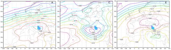
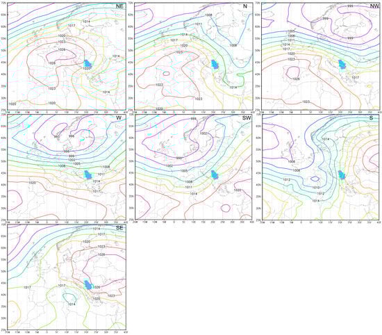
Figure 2.
Long-term mean of sea level pressure of each of the circulation types, two vorticity and eight pure directional types that affected Serbia in winter during the period 1961–2010.
In the anticyclonic (A) type, the centre lies over Serbia, while the cyclonic (C) type includes days with the lowest pressure southwest of Serbia. In the eastern (E) type, high pressure settled over Central Europe, with low pressure over the Greek islands. The north-eastern (NE) type is characterised by high pressure, which extends from the Atlantic across western and central Europe to the east. The northern (N) type is characterised by a low over Eastern Europe and high pressure over south-western Europe with a centre over Spain. The northwestern (NW) type is characterised by a low over north-eastern Europe with a large area of high pressure over south-western Europe. The western (W) type is characterised by very low pressure that settles over northern Europe. In the southwestern (SW) type, the synoptic situation is characterised by a low over north-western Europe in the south. The southern (S) cases are characterised by low pressure west of Serbia and high pressure in the east. The centre of the southeastern (SE) type cyclone is located over the centre of the Mediterranean, while the high pressure is located northeast of Serbia.
3.1.1. Frequencies of Circulation Types
After categorising the 18,262 days of the study period using the method of Jenkinson and Collison, the seasonal (Table 2) frequencies of the various WTs were calculated.
Table 2.
Seasonal relative frequencies (%) of 10 circulation types.
Of the 10 circulation types, the A types were the most common in all seasons (Table 2), with the highest frequency of 31.54% in autumn. The C type reached its highest frequency of 18.67% in spring, followed by 16.64% in winter. The NE type had the highest frequency (21.33%) of all pure directional types in summer. The E type had the highest frequencies of 15.11%, 13.12% and 12.55% in summer, winter and autumn, respectively. In spring, the NE type (9.87%) was the most common of all pure directional types.
3.1.2. Trend of Circulation Weather Types
Table 3 shows the results of the trend analysis performed for the 10 circuit WTs. The trend coefficients for the A type were significant at the 5% level and showed a negative trend in summer and autumn. The trend coefficients for the C, NE and SE types were not significant at the 5% level, while the E and SW types showed a positive and negative trend in summer, respectively. Both the N and S types showed a decreasing trend in winter and summer. The frequency of the NW type showed a negative trend in spring, summer and autumn. A significant negative trend was observed for the W type in summer and autumn.
Table 3.
Trend coefficient of the circulation types during the period 1961–2010 in Serbia.
3.2. Relationship Between Circulation Types and Temperature in Serbia
3.2.1. Trends of Mean, Maximum and Minimum Temperatures
The results of the trend analysis for the temperatures at six stations are shown in Table 4. The trend coefficients for mean temperature were significant at the 5% level and showed a positive trend for summer and spring (except Niš) and in winter in Negotin, Zlatibor and Zrenjanin. showed a significant positive trend for winter (except Negotin), summer (except Loznica) and spring at all stations. showed a significant positive trend for summer in Niš, Loznica and Negotin and for spring in Negotin. In autumn, the trend coefficients for all temperatures (T, and ) were not significant at the 5% level.
Table 4.
Trend coefficient of the mean, maximum and minimum temperatures during the period 1961–2010 in Serbia.
3.2.2. Mean, Maximum and Minimum Temperatures for Circulation Types
The T, and for six stations for all types in winter are shown in Table 5. The lowest temperatures were recorded for all stations when the E type prevailed over Serbia, except for Negotin, where the lowest temperatures were recorded when the SE type prevailed over Serbia. In addition to the E and SE types, the NE type was associated with “cold” conditions, while the highest temperatures were recorded for the SW, W and NW types. The differences between the A and C types for T and were negligible. In Zrenjanin, for example, the difference was −0.4 °C for T and 0.2 °C for . The during the A type was on average 2 °C or 3 °C lower than during the C type.
Table 5.
Mean (T), maximum () and minimum () temperatures for 10 circulation types and 6 stations for period 1961–2010 for winter.
T and reached their highest values in Belgrade (8.6 °C and 4.1 °C, respectively), while was highest in Loznica (13.5 °C), during the presence of the SW type over Serbia. Conversely, T, and were lowest in Zlatibor (−6.6 °C, −3.7 °C and −8.3 °C, respectively) when the E type occurred. These results were not surprising, as Zlatibor is the highest. However, it should be noted that it is colder in Negotin during the S and SW types than in Zlatibor, even though it is at a much lower altitude.
T and showed maximum values for all stations during the SW type, except in Negotin (maximum values during the NW and N type) in spring (Table S1). The highest was recorded during W type over Serbia. Minimum temperatures were associated with E type, except in Negotin. Temperatures were lowest in Negotin when the SE type was over Serbia.
Temperatures were highest when the S and SW types dominated over Serbia in summer (Table 6), except in Negotin. The weather was warmest during the E type in Negotin. The N type had the coldest conditions at almost all stations, except in Loznica, where it was coldest during the C type. The highest T and in Belgrade were 24.1 °C (for the S type) and 18.3 °C (for the S type), respectively. The highest was 30.9 °C in Niš. The lowest temperatures were recorded in Zlatibor.
Table 6.
Mean (T), maximum () and minimum () temperatures for 10 circulation types and 6 stations for period 1961–2010 for summer.
The temperature values were highest when the SW type was over Serbia in autumn (Table S2). Again, Negotin showed unique results, with temperatures peaking during the NW or N types. The lowest values varied depending on the station and the specific types. Similar to the winter months, temperatures in Negotin were lower than in Zlatibor during the S and SW types.
3.2.3. Temperature Anomalies
The temperature anomalies were calculated for all seasons and six stations for the period 1961–2010. Table 7 shows the anomalies for winter, while Tables S3–S5 show the anomalies for spring, summer and autumn, respectively. The largest positive anomalies of air temperature were observed during the SW type at all stations in winter, spring (T and ) and autumn (T and ), except in Negotin for all seasons, in Niš and Loznica for in autumn and in Niš, Zlatibor and Loznica for in spring. The anomalies of T, and showed the highest values in Negotin during the W, NW or N types, depending on the three seasons mentioned above. Conversely, the largest negative temperature anomalies occurred in winter and spring for the E or SE types at all stations. In autumn, the largest negative anomalies of T and were observed when C or E types were over Serbia, and for during the SE type. In summer, the largest positive temperature anomalies were found during the S or SW types, while the largest negative anomalies were generally observed during the N type.
Table 7.
Anomalies of mean (T), maximum () and minimum () temperatures for 10 circulation types and 6 stations for period 1961–2010 for winter.
3.2.4. Stepwise Regression
The results for the multilinear regression with stepwise procedure are shown in Table 8. The best results were obtained for winter, with several stations in other seasons having predictors excluded from the LRM (indicated by the symbol “/” in the table) due to significance levels exceeding 0.05. The models for T and were better than the models for . The highest correlation coefficients and NSE were found for Loznica (0.65 and 0.3) and Zlatibor (0.64 and 0.28) for mean temperatures in winter (Table 8). Figure 3 presents scatter plots between observed and modelled mean temperatures for these stations to provide a clearer illustration of the model’s performance. The plots indicate a moderate positive correlation between the observed and modelled temperatures. The predictors accepted in the winter models for T, and are shown in Figure 4 for each station.
Table 8.
Results from stepwise regression models.
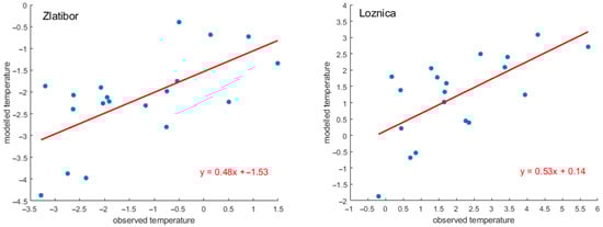
Figure 3.
Comparison between observed and modelled mean winter temperatures for the 1991–2010 period, derived using stepwise regression, for Zlatibor (left) and Loznica (right). The linear regression line is shown on each plot.
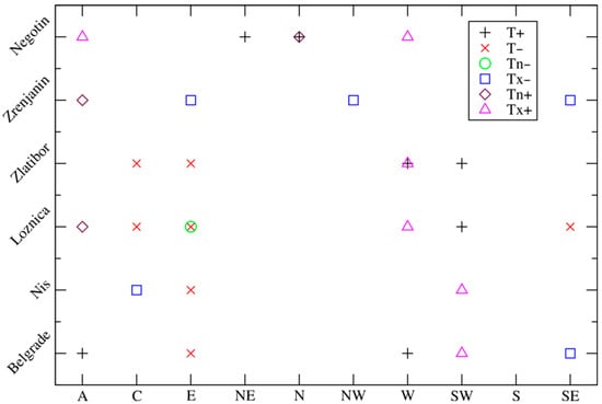
Figure 4.
Predictors accepted in the models for six stations: (+) CTs have positive coefficients in stepwise models for T, (×) CTs have negative coefficients for T, (○) CTs have negative coefficients for , (□) CTs have negative coefficients for , (◊) CTs have positive coefficients for and (Δ) CTs have positive coefficients for .
The E type frequently appeared in models with negative coefficients, followed by the A and W types with positive coefficients. The SW type had a positive coefficient and appeared four times in equations. The C and SE types had negative coefficients and were accepted three times each. The N and NW types had positive and negative coefficients, respectively, while the S type did not appear in any of the equations. The LRMs with the most predictors (four) were accepted for Zlatibor and Loznica for the mean temperature.
4. Discussion
In this study, 10 circulating WTs were analysed over Serbia in the period 1961–2010 according to the method of Jenkinson and Collison. In addition, the study analysed the relationships between atmospheric circulation WTs and seasonal mean, maximum and minimum temperatures.
As far as the frequency of the 10 circulation types is concerned, a high percentage of type A was found for all seasons. The second most frequent type was C for winter and spring and NE/E for summer/autumn. The A type was found to be the most common for different regions in Europe [38,39,40].
The decreasing trend in the frequency of A types corresponded with the increasing trend in daily minimum temperature, a result consistent with the findings of [41]. The temperature trends were highest in summer. With the exception of autumn, the trend coefficients for maximum temperatures exceeded those for minimum temperatures in all seasons. These results indicate that the mean temperature is more strongly influenced by the maximum temperature than by the minimum temperature. Unkašević et al. [42] have already found that the increase in mean summer temperatures in Belgrade in the period 1975–2003 was associated with a significant increase in the occurrence of extreme maximum temperatures. The decreasing trend in the frequency of type A circulations confirms that changes in atmospheric circulation in the middle troposphere, especially those affecting anticyclones, are one of the main causes of the increasingly warmer summer nights in Serbia in recent decades. Tošić et al. [43] recorded an increase in minimum temperature-based indices (daily minimum temperature, coldest nights, warm nights, tropical nights) for Serbia. The highest increase was observed for warm nights during the summer season.
The relationship between temperatures and types of atmospheric circulation was studied by analysing the mean values and anomalies of temperature for each type of atmospheric circulation. This study showed that temperatures in winter were highest in the SW circulation and lowest in the E circulation over Serbia. Mean temperatures were significantly higher in Belgrade, most likely due to the phenomenon of the urban heat island effect, which explains higher air temperatures in cities compared to their immediate surroundings. Negotin had both the highest and lowest temperatures to differentiate the types from the rest of Serbia. The geographical location and the characteristics of the relief led to certain climatic peculiarities in Negotin. This station is located in a basin surrounded by higher mountain ranges (Figure 1), which reduces the influence of air masses from other parts of the country. In addition, the influence of the oceanic and Mediterranean climate, which is typical for a large part of Serbia, is significantly weaker in this area. Winter temperatures in Negotin may differ from those at other stations due to temperature inversions that occur during anticyclones and affect local temperature conditions. Although Negotin is at the lowest altitude and Zlatibor at the highest, temperatures in Negotin during SW and S types were lower than in Zlatibor. This is due to the fact that the whole of Serbia is under the influence of cyclonic circulation, which brings warm air from the south, with the exception of eastern Serbia (Negotin), which is influenced by the back of the anticyclone over Eastern Europe.
In winter, the largest positive anomalies in air temperatures (T, and ) occurred during the southwestern zonal circulation for all stations except in Negotin (during the NW type). The SW type leads to positive anomalies because warm air masses are transported from the Mediterranean region to Serbia in winter. The positive temperature anomalies were higher in winter than in the other seasons. Przybylak and Maszewski [44] found that atmospheric circulation exerts the greatest influence on air temperature in the cold half of the year, when the solar factor is significantly weakened. During this period, the air temperature changes are mainly caused by the advection of air masses with different physical properties. In this study, the largest negative air temperature anomalies were observed during the eastern zonal circulation type. These anomalies are attributed to the anticyclonic thermal situation north of Serbia.
In this study, stepwise regression was applied to validate the potential predictors and to establish links between the predictors (circulation types) and the predictands (air temperatures). The validation results for the period 1991–2010 using stepwise regression indicated that the statistical prediction model was appropriate for the mean temperature for Zlatibor and Loznica and for the maximum temperature for Belgrade, Niš and Negotin in winter. For other seasons and stations, however, this model did not prove to be equally reliable. Our results are in agreement with the observations of [18]. They found that the results of the stepwise regression model provide more accurate estimates in the winter months than in the summer. Nonetheless, although the winter models for mean temperature in Zlatibor and Loznica demonstrated a reasonable ability to capture observed temperature variability, the regression slope being less than one suggests a systematic bias—namely, the underestimation of higher temperatures and the overestimation of lower ones. This indicates a need for further model refinement, particularly with regard to the representation of extreme temperature values. Buishand and Brandsma [45] have also emphasised that Jenkinson and Collison’s method performs relatively poorly for temperature. This could be due to the non-use of data from the upper air layer in this scheme. While changes in observed temperature cannot always be explained by changes in large-scale atmospheric circulation patterns alone, investigating the relationship between temperature and circulation is crucial for understanding temperature variability and developing circulation-based downscaling methods [46]. It is important to recognise that stepwise regression methods tend to produce biased coefficient estimates, underestimated standard errors, multicollinearity among predictors, and spuriously low p-values because the variables are selected from the same data set used for model fitting [47]. The exclusive use of surface-level circulation types without including information from the upper air layer (e.g., geopotential height at 500 hPa) ignores critical vertical atmospheric structures that modulate temperature, such as persistent anticyclonic patterns and thermal advection. In addition, the influence of surface circulation types can vary significantly over the seasons; therefore, models that do not account for seasonal interactions risk producing biased or misleading results. These methodological limitations emphasise the importance of integrating upper-air variables, SST, moisture indices and large-scale teleconnection patterns (e.g., NAO, EA, EA/WR) to improve the meteorological relevance and predictive performance of circulation-based temperature models.
5. Conclusions
To summarise, this study elucidates the effects of circulation WTs on temperatures in Serbia. From the results, it can be deduced that the A type occurs most frequently in Serbia. The warmest weather occurs when the SW type is over Serbia, in all seasons. Types C, E and N caused the lowest temperatures depending on the season. The WTs were successfully used as potential predictors for some winter temperatures, while the models proved inadequate for other seasons.
The results of this study can be used to improve the seasonal forecasting models and for predicting extreme events in Serbia. More accurate results could possibly be obtained by including additional predictors, such as pressure at different altitudes, wind patterns and teleconnection indices. These predictors could also be integrated into alternative statistical or machine learning methods (e.g., LASSO and Random Forest), which could be explored in future research.
Supplementary Materials
The following supporting information can be downloaded at: https://www.mdpi.com/article/10.3390/atmos16080969/s1, Figure S1: Long-term mean of sea level pressure of each of the then circulation types, two vorticity and eight pure directional types that affected Serbia in spring during the period 1961–2010; Figure S2: Long-term mean of sea level pressure of each of the then circulation types, two vorticity and eight pure directional types that affected Serbia in summer during the period 1961–2010; Figure S3: Long-term mean of sea level pressure of each of the then circulation types, two vorticity and eight pure directional types that affected Serbia in autumn during the period 1961–2010; Table S1: Mean (T), maximum () and minimum () temperatures for 10 circulation types and 6 stations for period 1961–2010 for spring; Table S2: Mean (T), maximum () and minimum () temperatures for 10 circulation types and 6 stations for period 1961–2010 for autumn; Table S3: Anomalies of mean (T), maximum () and minimum () temperatures for 10 circulation types and 6 stations for period 1961–2010 for spring; Table S4: Anomalies of mean (T), maximum () and minimum () temperatures for 10 circulation types and 6 stations for period 1961–2010 for summer; Table S5: Anomalies of mean (T), maximum () and minimum () temperatures for 10 circulation types and 6 stations for period 1961–2010 for autumn.
Funding
This research was supported by the Science Fund of the Republic of Serbia, No. 7389, Project: “Extreme weather events in Serbia—analysis, modelling and impacts”—EXTREMES.
Institutional Review Board Statement
Not applicable.
Informed Consent Statement
Not applicable.
Data Availability Statement
Data is contained within the article and Supplementary Materials.
Acknowledgments
The author would like to thank the Hydrometeorological Service of Serbia, which provided the data necessary for this study.
Conflicts of Interest
The author declares no conflicts of interest.
References
- Ustrnul, Z.; Wypych, A.; Winkler, A.J.; Czekierda, D. Late spring freezes in Poland in relation to atmospheric circulation. Quaest. Geogr. 2014, 33, 165–172. [Google Scholar] [CrossRef][Green Version]
- Lamb, H.H. British Isles Weather Types and a Register of Daily Sequence of Circulation Patterns, 1861–1971; Stationery Office Books: London, UK, 1972; p. 88. [Google Scholar]
- Jenkinson, A.F.; Collison, F.P. An initial climatology of gales over the North Sea. Synop. Climatol. Branch Memo. 1977, 62, 18. [Google Scholar]
- Jones, P.D.; Hulme, M.; Briffa, K.R. A comparison of Lamb circulation types with an objective classification scheme. Int. J. Climatol. 1993, 13, 655–663. [Google Scholar]
- Fernández-Granja, J.A.; Brands, S.; Bedia, J.; Casanueva, A.; Fernández, J. Exploring the limits of the Jenkinson–Collison weather types classification scheme: A global assessment based on various reanalyses. Clim. Dyn. 2023, 61, 1829–1845. [Google Scholar] [CrossRef]
- Huth, R.; Beck, C.; Philipp, A.; Demuzere, M.; Ustrnul, Y.; Cahynová, M.; Kyselý, J.; Tveito, O.E. Classifications of atmospheric circulation patterns: Recent advances and applications. Ann. N. Y. Acad. Sci. 2008, 1146, 105–152. [Google Scholar] [PubMed]
- Sheridan, C.S.; Lee, C.C. The self-organizing map in synoptic climatological research. Prog. Phys. Geog. 2011, 35, 109–119. [Google Scholar]
- Jiang, N.; Cheung, K.; Luo, K.; Beggs, P.J.; Zhou, W. On two different objective procedures for classifying synoptic weather types over east Australia. Int. J. Climatol. 2012, 32, 1475–1494. [Google Scholar]
- Mittermeier, M.; Weigert, M.; Rügamer, D.; Küchenhoff, H.; Ludwig, R. A deep learning based classification of atmospheric circulation types over Europe: Projection of future changes in a CMIP6 large ensemble. Environ. Res. Lett. 2022, 17, 084021. [Google Scholar] [CrossRef]
- IPCC. Climate Change 2021: The Physical Science Basis. Contribution of Working Group I to the Sixth Assessment Report of the Intergovernmental Panel on Climate Change; Masson-Delmotte, V., Zhai, P., Pirani, A., Connors, S.L., Péan, C., Berger, S., Caud, N., Chen, Y., Goldfarb, L., Gomis, M.I., et al., Eds.; Cambridge University Press: Cambridge, UK; New York, NY, USA, 2021; 2391p. [Google Scholar]
- Kyselý, J. Temporal fluctuations in heat waves at Prague–Klementinum, the Czech Republic, from 1901–1997, and their relationships to atmospheric circulation. Int. J. Climatol. 2002, 22, 33–50. [Google Scholar]
- Domonkos, P.; Kyselý, J.; Piotrowicz, K.; Petrovic, P.; Likso, T. Variability of extreme temperature events in south-central Europe during the 20th century and its relationship with large scale circulation. Int. J. Climatol. 2003, 23, 987–1010. [Google Scholar]
- Corte-Real, J.; Zhang, X.; Wang, X. Large-scale circulation regimes and surface climatic anomalies over the Mediterranean. Int. J. Climatol. 1995, 15, 1135–1150. [Google Scholar] [CrossRef]
- Kutiel, H.; Maheras, P. Variations in the Temperature Regime Across the Mediterranean During the Last Century and their Relationship with Circulation Indices. Theor. Appl. Climatol. 1998, 61, 39–53. [Google Scholar] [CrossRef]
- Maheras, P.; Kutiel, H. Spatial and temporal variations in the themerature regime in the Mediterranean and their relationship with circulation during the last century. Int. J. Climatol. 1999, 19, 745–764. [Google Scholar] [CrossRef]
- Maheras, P.; Xoplaki, E.; Kutiel, H. Wet and dry monthly anomalies across the Mediterranean basin and their relationship with circulation, 1860–1990. Theor. Appl. Climatol. 1999, 64, 189–199. [Google Scholar] [CrossRef]
- Feidas, H.; Makrogiannis, T.; Bora-Senta, E. Trend analysis of air temperature time series in Greece and their relationship with circulation using surface and satellite data: 1955–2001. Theor. Appl. Climatol. 2004, 79, 185–208. [Google Scholar] [CrossRef]
- Peña-Angulo, D.; Trigo, R.M.; Cortesi, N.; González-Hidalgo, J.C. The influence of weather types on the monthly average maximum and minimum temperatures in the Iberian Peninsula. Atmos. Res. 2016, 178-179, 217–230. [Google Scholar] [CrossRef]
- Pérez, I.A.; García, Á. Climate change in the Iberian Peninsula by weather types and temperature. Atmos. Res. 2023, 284, 106596. [Google Scholar] [CrossRef]
- Vera, C.; Vigliarolo, K.P. A Diagnostic Study of Cold-Air Outbreaks over South America. Mon. Weather Rev. 2000, 128, 3–24. [Google Scholar] [CrossRef]
- Vera, C.; Vigliarolo, K.P.; Berbery, H.E. Cold season synoptic-scale waves over subtropical South America. Mon. Weather Rev. 2002, 130, 684–699. [Google Scholar] [CrossRef]
- Solman, S.A.; Menéndez, C.G. Weather regimes in the South American sector and neighbouring oceans during winter. Clim. Dyn. 2003, 21, 91–104. [Google Scholar] [CrossRef]
- Espinoza, C.J.; Ronchail, J.; Lengaigne, M.; Quispe, N.; Silva, Y.; Bettolli, L.M.; Avalos, G.; Llacza, A. Revisiting wintertime cold air intrusions at the east of the Andes: Propagating features from subtropical Argentina to Peruvian Amazon and relationship with large-scale circulation patterns. Clim. Dyn. 2013, 41, 1983–2002. [Google Scholar] [CrossRef]
- Unkašević, M.; Tošić, I. The maximum temperatures and heat waves in Serbia during the summer of 2007. Clim. Change 2011, 108, 207–223. [Google Scholar] [CrossRef]
- Unkašević, M.; Tošić, I. Trends in temperature indices over Serbia: Relationships to large-scale circulation patterns. Int. J. Climatol. 2013, 33, 3152–3161. [Google Scholar] [CrossRef]
- Ruml, M.; Gregorić, E.; Vujadinović, M.; Radovanović, S.; Matović, G.; Vuković, A.; Počuča, V.; Stojičić, Đ. Observed changes of temperature extremes in Serbia over the period 1961−2010. Atmos. Res. 2017, 183, 26–41. [Google Scholar] [CrossRef]
- Tošić, I.; Putniković, S.; Tošić, M.; Lazić, I. Extreme Temperature Events in Serbia in Relation to Atmospheric Circulation. Atmosphere 2021, 12, 1584. [Google Scholar] [CrossRef]
- Putniković, S.; Tošić, I.; Ðurđević, V. Circulation weather types and their influence on precipitation in Serbia. Meteorol. Atmos. Phys. 2016, 128, 649–662. [Google Scholar] [CrossRef]
- Putniković, S.; Tošić, I. Relationship between atmospheric circulation weather types and seasonal precipitation in Serbia. Meteorol. Atmos. Phys. 2018, 130, 393–403. [Google Scholar] [CrossRef]
- Unkašević, M.; Tošić, I. Changes in extreme daily winter and summer temperatures in Belgrade. Theor. Appl. Clim. 2009, 95, 27–38. [Google Scholar] [CrossRef]
- Mihailović, D.T.; Lalić, B.; Drešković, N.; Mimić, G.; Djurdjević, V.; Jančić, M. Climate change effects on crop yields in Serbia and related shifts of Köppen climate zones under the SRES-A1B and SRES-A2. Int. J. Clim. 2015, 35, 3320–3334. [Google Scholar] [CrossRef]
- Alexandersson, H. A homogeneity test applied to precipitation data. J. Climatol. 1986, 6, 661–675. [Google Scholar] [CrossRef]
- Jones, P.D.; Harpham, C.; Briffa, K.R. Lamb weather types derived from Reanalysis products. Int. J. Climatol. 2013, 33, 1129–1139. [Google Scholar] [CrossRef]
- Ramos, A.; Sprenger, M.; Wernli, H.; Duran-Quesada, A.; Lorenzo, M.; Gimeno, L. A new circulation type classification based upon Lagrangian air trajectories. Front. Earth Sci. 2014, 2, 29. [Google Scholar] [CrossRef]
- Kalnay, E.; Kanamitsu, M.; Collins, W.; Deaven, D.; Gandin, L.; Iredell, M.; Sahs, S.; White, G.; Woollen, J.; Leetmaa, Z.A.; et al. The NCEP/NCAR 40-year reanalysis project. Bull. Am. Meteorol. Soc. 1996, 77, 437–470. [Google Scholar] [CrossRef]
- Huth, R. Statistical downscaling in central Europe: Evaluation of methods and potential predictors. Clim. Res. 1999, 13, 91–101. [Google Scholar] [CrossRef]
- Goyal, M.R.; Ojha, C.S.P. Evaluation of various linear regression methods for downscaling of mean monthly precipitation in arid Pichola watershed. Nat. Resour. 2010, 1, 11–18. [Google Scholar] [CrossRef]
- Trigo, R.M.; DaCamara, C.C. Circulation weather types and their influence on the precipitation regime in Portugal. Int. J. Climatol. 2000, 20, 1559–1581. [Google Scholar] [CrossRef]
- Linderson, M.L. Objective classification of atmospheric circulation over southern Scandinavia. Int. J. Climatol. 2001, 21, 155–169. [Google Scholar] [CrossRef]
- Spellman, G. An assessment of the Jenkinson and Collison synoptic classification to a continental mid-latitude location. Theor. Appl. Climatol. 2017, 128, 731–744. [Google Scholar] [CrossRef]
- Radinović, Ð. Weather and climate in Yugoslavia; IRO Građevinska knjiga: Belgrade, Serbia, 1981; p. 423. (In Serbian) [Google Scholar]
- Unkašević, M.; Vujović, D.; Tošić, I. Trends in extreme summer temperatures at Belgrade. Theor. Appl. Climatol. 2005, 82, 99–205. [Google Scholar] [CrossRef]
- Tošić, I.; Tošić, M.; Lazić, I.; Aleksandrov, N.; Putniković, S.; Djurdjević, V. Spatio-temporal changes in the mean and extreme temperature indices for Serbia. Int. J. Climatol. 2023, 43, 2391–2410. [Google Scholar] [CrossRef]
- Przybylak, R.; Maszewski, R. Influence of atmospheric circulation on air temperature and precipitation in the Bydgoszcz–Toruń region in the period from 1921 to 2000. Bull. Geog. Phys. Geog. Ser. 2009, 1, 19–37. [Google Scholar] [CrossRef][Green Version]
- Buishand, A.; Brandsma, T. Comparison of circulation classification schemes for predicting temperature and precipitation in the Netherlands. Int. J. Climatol. 1997, 17, 875–889. [Google Scholar] [CrossRef]
- Xoplaki, E.; González-Rouco, J.; Luterbacher, J.; Wanner, H. Mediterranean summer air temperature variability and its connection to the large-scale atmospheric circulation and SSTs. Clim. Dyn. 2003, 20, 723–739. [Google Scholar] [CrossRef]
- Wilks, D.S. Statistical Methods in the Atmospheric Sciences, 3rd ed.; Academic Press: San Diego, CA, USA, 2011; p. 676. [Google Scholar]
Disclaimer/Publisher’s Note: The statements, opinions and data contained in all publications are solely those of the individual author(s) and contributor(s) and not of MDPI and/or the editor(s). MDPI and/or the editor(s) disclaim responsibility for any injury to people or property resulting from any ideas, methods, instructions or products referred to in the content. |
© 2025 by the author. Licensee MDPI, Basel, Switzerland. This article is an open access article distributed under the terms and conditions of the Creative Commons Attribution (CC BY) license (https://creativecommons.org/licenses/by/4.0/).