Unveiling PM_2.5 Transport Pathways: A Trajectory-Channel Model Framework for Spatiotemporally Quantitative Source Apportionment

Abstract

In this study, we introduced a novel Trajectory-Channel Transport Model (TCTM) to unravel spatiotemporal dynamics of PM_2.5 pollution. By integrating high-resolution simulations from the Weather Research and Forecasting (WRF) model with the Nested Air-Quality Prediction Modeling System (WRF-NAQPMS) and 72 h backward-trajectory analysis, TCTM enables the precise identification of source regions, the delineation of key transport corridors, and a quantitative assessment of regional contributions to receptor sites. Focusing on four Yangtze River Delta cities (Hangzhou, Shanghai, Nanjing, Hefei) during a January 2020 pollution event, the results demonstrate that TCTM’s Weighted Concentration Source (WCS) and Source Pollution Characteristic Index (SPCI) outperform traditional PSCF and CWT methods in source-attribution accuracy and resolution. Unlike receptor-based statistical approaches, TCTM reconstructs pollutant transport processes, quantifies spatial decay, and assigns contributions via physically interpretable metrics. This innovative framework offers actionable insights for targeted air-quality management strategies, highlighting its potential as a robust tool for pollution mitigation planning.

1. Introduction

Air pollution remains a critical environmental challenge worldwide [1], with frequent severe episodes [2,3] that inflict significant harm on human health and ecosystems [4,5,6]. China’s rapid industrialization and urbanization over recent decades have exacerbated air-quality problems across the country [7,8,9]. In response, Chinese authorities have enacted stringent air-quality regulations and implemented aggressive emission-control measures at national, provincial, and municipal levels. Against this backdrop, the precise identification of pollution source regions and transport pathways is indispensable for devising effective prevention and mitigation strategies.

Currently, numerical air-quality models, such as AERMOD [10], CMAQ [11], CAMx [12], WRF-Chem [13], and NAQPMS [14], have achieved high-resolution simulations with multi-scale, multi-process, and multi-pollutant characteristics. These models generate gridded concentration datasets with high spatiotemporal resolution, enabling detailed analyses of pollutant formation, transport, transformation, and deposition processes [15]. As a result, they have seen widespread application in both academic research and operational forecasting [16,17,18]. For example, Zhang et al. [19] conducted AERMOD to quantify the average concentrations of PM_2.5 and CO attributable to primary vehicle emissions in Macau. Cheng et al. [20] used CAMx to evaluate the impact of emission-control policies on Beijing’s PM_2.5 levels; Wang et al. [21] combined CMAQ and CAMx to characterize regional PM_2.5 transport into Taizhou; Liu et al. [22] applied WRF-Chem to investigate the vertical profile of PM_2.5 during a severe Nanjing pollution event; and Hu et al. [23] examined basin-scale PM_2.5 transport in the Twai-Hu region. Similarly, Wang et al. [24] and Liu et al. [25] leveraged NAQPMS to simulate and apportion winter PM_2.5 in Beijing. Within these models, tracer-based source-apportionment modules—such as SOEM [26], ISAM [27], OSAM [28], and PSAT [29]—track specified emissions through atmospheric processes by embedding virtual tracers and solving mass-balance equations to quantify each source’s contribution to ambient concentrations [30]. While highly accurate, these techniques entail substantial computational cost, lengthy runtime, and specialized expertise, limiting their utility for rapid, operational air-quality management [31].

In contrast, HYSPLIT [32] is a Lagrangian atmospheric dispersion model that employs gridded meteorological data to simulate and trace atmospheric pollutant transport. It has been widely applied in source-region analysis and air-mass trajectory tracking [33,34]. HYSPLIT incorporated two receptor-oriented diagnostic tools—namely the Potential Source Contribution Function (PSCF) and the Concentration-Weighted Trajectory (CWT) methods—offer expedient, user-friendly means to infer potential source regions and transport pathways using backward trajectories and observed receptor concentrations [35,36,37]. PSCF computes, for each grid cell, the conditional probability that trajectories passing through that cell arrive at the receptor above a chosen concentration threshold [38], whereas CWT estimates the mean receptor concentration associated with air masses traversing each cell, weighted by residence time [39]. Although widely applied [40,41], these approaches remain inherently qualitative: they neither reconstruct the detailed transport process nor yield quantitative source contributions, and they can struggle to distinguish source importance when cells exhibit similar values [42,43,44,45]. Furthermore, the PSCF and CWT receptor models establish connections by assigning values based on the concentrations at the receptor site in conjunction with backward trajectories, rather than reconstructing the atmospheric transport processes, and only performing a qualitative identification of potential sources and directions through statistical analysis [42]. Specifically, the PSCF [43] calculated the probability of pollution trajectories, qualitatively identifying the main potential sources and directions; it does not reflect the magnitude of impact or the quantitative contribution to the receptor site. Similarly, the CWT [44] qualitatively assessed potential sources and was highly dependent on receptor concentrations, and could not accurately reflect regional pollution levels.

Therefore, to overcome the limitations existing methods, we developed a Trajectory-Channel Transport Model (TCTM), by integrating concentration fields with a trajectory analysis method. First, backward trajectories can be calculated using multi-source meteorological data (including meteorological reanalysis data or numerical simulations), while simultaneously extracting meteorological parameters at trajectory points. Concurrently, pollutant concentrations are obtained through the spatiotemporal matching of historical observations, reanalysis data, or numerical simulations along the trajectory points. By leveraging multi-source data integration, TCTM provides a flexible and robust solution for pollutant source tracing. Consequently, the TCTM demonstrates strong universality and facilitates widespread application, serving as a standardized post-processing analysis tool for atmospheric transport analysis. The primary objectives of TCTM are to rapidly and accurately identify potential source regions, determine key pollution transport pathways, and quantitatively assess the potential contributions of different source regions.

To validate the feasibility, reliability, and accuracy of TCTM, we simulated a representative PM_2.5 pollution transport event from the Beijing–Tianjin–Hebei regions towards the Yangtze River Delta (YRD) during 26–29 January 2020. Four major cities—Hangzhou, Shanghai, Nanjing, and Hefei—serve as receptor sites. For 29 January, we computed 72 h backwards trajectories (00:00–23:00 LST), applied PSCF and CWT for benchmarking, and compared their source-attribution results against TCTM’s WCS (Weighted Concentration Source) and SPCI (Source Pollution Characteristic Index) metrics. The remainder of this paper is organized as follows: Section 2.1 details the configuration and execution of the WRF-NAQPMS simulations; Section 2.2 describes the TCTM framework and derivation of WCS and SPCI; Section 3.1 analyzes the PM_2.5 pollution event and backward-trajectory origins; Section 3.2 presents the potential-source identification results and validates TCTM against PSCF/CWT; Section 3.3 quantifies transport contributions from the identified source regions.

2. Materials and Methods

2.1. Model Setup and Databases

The WRF model was driven by the global final analysis (FNL) data provided by the National Centers for Environmental Prediction (NCEP), with a 1° × 1° spatial resolution and 6 h temporal resolution (http://rda.ucar.edu/datasets/ds083.2/ (accessed on 23 to 31 January 2020)). In the WRF atmospheric process simulation, the physical parameterization schemes included the WSM3 microphysics scheme, Dudhia shortwave radiation scheme, Rapid Radiative Transfer Model (RRTM) for longwave radiations, Monin–Obukhov surface-layer scheme, Noah-MP land-surface process scheme, Yonsei University planetary-boundary-layer scheme, and Kain–Fritsch (KF) for the cumulus cloud parameterization scheme.

The NAQPMS model was developed by the Institute of Atmospheric Physics, Chinese Academy of Sciences [46,47,48]. It can simulate emissions, transport, chemical transformations, and the dry/wet deposition of pollutants, incorporating physical transport as well as aqueous-phase, gas-phase, and heterogeneous-phase chemistry processes [49,50]. Gas-phase chemistry follows the Carbon-Bond Mechanism Z (CBM-Z) (71 species and 176 reactions) [51]. While aqueous-phase chemistry and inorganic aerosol processes use enhanced RADM2 and ISORROPIA1.7 mechanisms [52], respectively. Secondary organic aerosol formation follows Odum et al.’s [53] scheme for anthropogenic and biogenic precursors, and natural aerosol emissions (dust, sea salt) follow the mechanisms of Luo et al. [54] and Athanasopoulou et al. [55].

In this study, the model simulation domain covers central and eastern China on a 76 × 97 grids at 27 km horizontal resolution, includes the whole YRD. The coordinate system is Lambert projection, the upper and lower standard latitude lines are 23° N and 43° N, respectively, and the central longitude is (115° E, 33° N). More detailed settings and validation given in previous studies [56,57]. Therefore, the backward-trajectory calculations and PM_2.5 analysis data employed in the subsequent sections of this study were obtained from WRF-NAQPMS model simulations for the period spanning from 23 to 31 January 2020. Given that atmospheric pollutants are primarily distributed in the near-surface layer, the starting height for backward-trajectory calculations in this study was set at near-surface grid height to accurately trace pollution sources and authentically reflect transport processes.

2.2. Research Methods

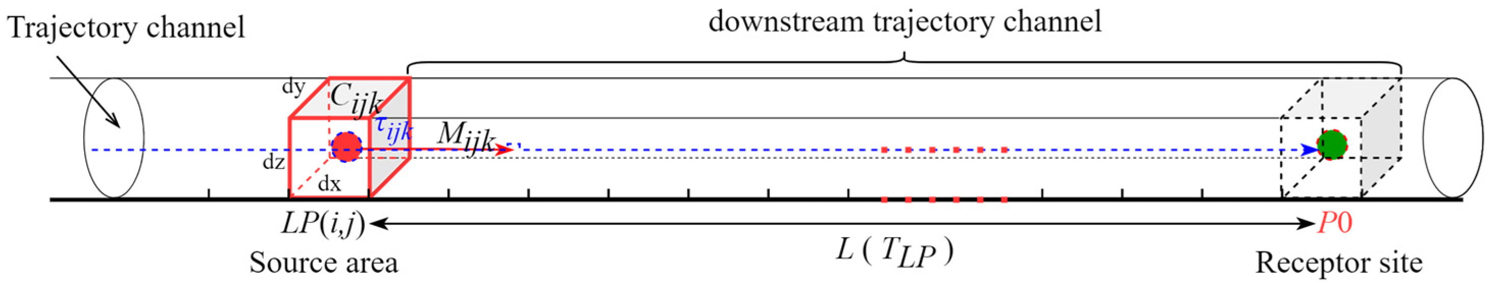
2.2.1. Trajectory-Channel Transport Model (TCTM)

Using the high spatial and temporal resolution meteorological data simulated by the WRF-NAQPMS model, we calculated 72 h backward trajectories and extracted the corresponding PM_2.5 concentrations and meteorological parameters to reconstruct pollutant transport from source regions to the receptor site. This approach established the Trajectory-Channel Transport Model (TCTM), a novel framework integrating trajectory analysis and transport diagnostics. This framework enables us to analyze regional PM_2.5 transport processes across defined pathways and quantified the contributions of regional transport to the receptor site.

Model Construction Principle: TCTM establishes a “trajectory channel” that links each source region to the receptor site via air-mass backward trajectories. It is assumed that all pollutant flux from a given source travels uniformly within this channel to the receptor. By simplifying three-dimensional atmospheric transport process into a one-dimensional Lagrangian transmission channel, TCTM allows for a straightforward quantitative analysis of regional pollutant contributions. Figure 1 illustrates the concept of TCTM, and the following section presents its mathematical derivation and governing Equations.

The total mass of PM_2.5 transported from source grid cell LP (i,j) along trajectory k during its residence time is given by:

$$M_{ijk}={\sum }_{\tau =1}^{{\tau }_{ijk}}{C}_{ijk\tau }·V_{ijk\tau }·S_{ijk\tau }.dt$$

(1)

where C_ijkτ is the PM_2.5 concentration, V_ijkτ is the wind speed, S_ijkτ is the cross-sectional area at grid cell (i,j) along trajectory k, respectively, and τ_ijk corresponds to the residence time (defined by the 1 h temporal resolution) at grid cell (i,j). The total volume of the transport channel from source cell LP (i,j) to receptor point P0 along trajectory k is denoted as:

$${VL}_{LP}={\sum }_{T=1}^{T_{LP}}{V}_{ijkT}·S_{ijkT}.dt$$

(2)

where V_ijkT and S_ijkT represent the wind speed and sectional area, respectively, at each segment T time along the trajectory channel. T_LP denotes the total transport time of trajectory k from source region LP (i,j) to the receptor point P0.

Based on the mass conservation principles between PM_2.5 emission from the source area and its accumulation in the downstream channel, the regional PM_2.5 transport contribution from source grid LP (i,j) to the receptor point P0 is defined as the mean concentration increment within the channel trajectory k, denoted as ∆C_ijk, based on the fundamental Equations (1) and (2):

$${\mathsf{\Delta }C}_{ijk}={\displaystyle \frac{M_{ijk}}{{VL}_{LP}}}$$

(3)

Expanding Equation (3) using Equations (1) and (2) gives us:

$${\mathsf{\Delta }C}_{ijk}={\displaystyle \frac{{\sum }_{\tau =1}^{{\tau }_{ijk}}{C}_{ijk\tau }·V_{ijk\tau }·S_{ijk\tau }}{{\sum }_{T=1}^{T_{LP}}{V}_{ijkT}·S_{ijkT}}}$$

(4)

Assuming uniform cross-sectional areas between source and receptor channels (S_ijkT ≈ S_ijkτ), Equation (4) can be simplified as follows:

$${\mathsf{\Delta }C}_{ijk}={\displaystyle \frac{{\sum }_{\tau =1}^{{\tau }_{ijk}}{C}_{ij\tau k}·V_{ij\tau k}.dt}{{\sum }_{T=1}^{T_{LP}}{V}_{ijkT}.dt}}$$

(5)

In Equation (5), ΣV_ijkτ$dt$ represents the source transmission impact distance l_ijk for grid cell (i,j), and Σ V_ijkT$dt$ corresponds to the total transport distance L from LP (i,j) to P0. Thus, Equation (5) can be rewritten as:

$${\mathsf{\Delta }C}_{ijk}={\displaystyle \frac{l_{ijk}}{L}}·C_{ijk}={\displaystyle \frac{{\tau }_{ijk}·V_{ijk}}{T_{LP}·Va}}·C_{ijk}$$

(6)

Equation (6), V_ijk and C_ijk are the average wind speed and PM_2.5 concentration at source grid cell (i,j) during its residence time τ_ijk, respectively, while V_a is the average transport speed of the air mass along the following channel k. The ratio of l_ijk/L can be interpreted as the Distance Transport Factor, R_ijk, reflecting spatial pollution decay with distance and time:

$$R_{ijk}={\displaystyle \frac{l_{ijk} }{L}}={\displaystyle \frac{{\tau }_{ijk}·V_{ijk}}{T_{LP}·Va}}$$

(7)

With R_ijk defined as in Equation (7), Equation (6) can thus be simplified to:

$${\mathsf{\Delta }C}_{ijk}=R_{ijk}·C_{ijk}$$

(8)

For N air-mass trajectories passing through the source region LP (i,j), the average contribution concentration to the receptor site P0 denoted as CCS_ij, is calculated by summing and averaging the incremental concentration ∆C_ijk (Equation (8)) across all N trajectories:

$${CCS}_{ij}={\displaystyle \frac{\sum _{k=1}^N{\mathsf{\Delta }C}_{ijk}}{N}}={\displaystyle \frac{\sum _{k=1}^N{R}_{ijk}·C_{ijk}}{N}}$$

(9)

The Trajectory-Channel Transport Model could physically capture the spatiotemporal decay of pollutant contributions from the source regions to the receptor site and quantify its contribution. To further assess the long-term transport impacts, we introduce the Weighted Concentration of Source (WCS), an indicator reflecting the potential regional influence to the receptor, which integrates the Distance Transport Factor R_ijk and receptor site concentration, using Equations (8) and (7):

$${WCS}_{ij}={\displaystyle \frac{\sum _{k=1}^N{R}_{ijk}·C_{P0k}·C_{ijk}}{\sum _{k=1}^N{R}_{ijk}·C_{P0k}}}$$

(10)

where C_P0k is the PM_2.5 concentration at receptor P0 for trajectory k. Based on the distribution of WCS values, one can evaluate comprehensive pollution levels and determine the impact of different air masses passing through source regions. To further assess the long-term transport potential from source regions, the Source Pollution Characteristic Index (SPCI) is defined as the ratio of the WCS to a pollution-level threshold, according to Equation (10) and not consider the weighted receptor concentration:

$${SPCI}_{ij}={\displaystyle \frac{{WCS}_{ij}}{{PM}_{lvl}}}={\displaystyle \frac{\sum _{k=1}^N{R}_{ijk}·C_{ijk}}{{PM}_{lvl}\sum _{k=1}^N{R}_{ijk}}}$$

(11)

In Equation (11), PM_lvl represents the threshold PM_2.5 pollution level, set as 75 µg·m⁻³ in this study. If the value of SPCI_ij > 1, it indicates that grid cell (i,j) is heavily polluted and significantly contributes to downstream trajectory channel and receptor site. Conversely, SPCI_ij < 1 suggests minimal or lighter regional transport contribution. Mapping areas with SPCI_ij > 1 enables the identification of major pollution sources and dominant transport pathways.

2.2.2. PSCF and CWT Methods

To validate the feasibility, reliability, and accuracy of the WCS and SPCI approaches for identifying potential source areas, we also applied two well-established receptor-oriented diagnostic tools: PSCF and CWT methods [44,58,59,60]. These classical methods serve to corroborate our trajectory-based source identification and localization. A comprehensive description of both PSCF and CWT can be found in [61]. The PSCF for grid cell (i,j) is defined as:

$${PSCF}_{ij}={\displaystyle \frac{m_{ij}}{n_{ij}}}$$

(12)

where m_ij is the number of pollution trajectories that both pass through the grid (i,j) and arrive at the receptor with PM_2.5 concentration above the chosen threshold (75 µg m⁻³), and n_ij is the total number of trajectories passing through the grid (i,j). The CWT for grid cell (i,j) is calculated by:

$${CWT}_{ij}={\displaystyle \frac{1}{{\sum }_{k=1}^N{\tau }_{ijk}}}\times \sum _{k=1}^N{C}_k{\tau }_{ijk}$$

(13)

where C_k is the observed PM_2.5 concentration upon the arrival of trajectory k at the receptor, τ_ijk is the residence time within the grid (i,j), and N is the total number of trajectories passing through the grid (i,j). Larger CWT_ij values imply that air masses traveling over grid (i,j) carry higher average PM_2.5 concentrations to the receptor, indicating stronger potential influence. By comparing the spatial patterns of PSCF, CWT, WCS, and SPCI, we achieve a robust cross-validation of the regions that are most likely to contribute to PM_2.5 pollution at our receptor sites.

3. Results

3.1. Regional Pollution Transportation Process of PM_2.5

The spatial migration of PM_2.5 concentrations across central and eastern China during 26–29 January 2020, and the air-mass backward trajectories arriving in key cities Hangzhou, Shanghai, Nanjing, and Hefei on 29 January 2020 were shown in Figure 2. There was a notable regional PM_2.5 transport from the Beijing–Tianjin–Hebei (BTH) to the YRD during this pollution episode (Figure 2a). On 26 January, stagnant meteorological conditions led to severe PM_2.5 pollution (>75 µg·m⁻³) in BTH, while the YRD remained unaffected due to clean air masses. By the 27th, the BTH continued to be affected by stable weather, resulting PM_2.5 accumulation increased and gradually slowly transported toward southeastern YRD. On the 28th, with the shift in the wind field in the BTH, the stable weather transitioned to northwesterly winds, facilitating PM_2.5 transport from the BTH through Henan to Anhui under the action of the northwest wind. Concurrently, the PM_2.5 concentrations increased in the YRD’s coastal areas. By the 29th, sustained northwesterly winds carried PM_2.5 pollution into northern Zhejiang, causing regional PM_2.5 pollution across Hangzhou, Shanghai, Nanjing, and Hefei.

Therefore, through analyzing the backward trajectories at different time points and regional transport variations of PM_2.5 (Figure 2a), as well as the vertical PM_2.5 distributions along clustered trajectories (Figure 2b–e), we elucidated the transport characteristics of PM_2.5 pollution in Hangzhou, Shanghai, Nanjing, and Hefei on the 29th.

In Hangzhou, backward-trajectory analysis (Figure 2b, blue trajectory) and associated vertical PM_2.5 distributions on the 29th revealed that air masses arriving in Hangzhou were primarily transported from central and southern Anhui within the 0–24 h period. The altitude of these air masses mostly remained below 500 m, crossing the Zhejiang boundary below 250 m, exhibiting consistent PM_2.5 pollution. On the 28th, the 12–36 h backward trajectory indicated transport from southeastern Henan to central–western Anhui. When the polluted air masses (at 500~600 m above Henan) were advected to Anhui, their altitude descended to 250~500 m, exacerbating PM_2.5 levels. For the 27th, the 36–60 h backward trajectory primarily passed over eastern Henan at height of 600~800 m. Overall, these air masses remained relatively clean, except near the borders with Shandong and Henan, where they were affected by southward diffusion pollution from the BTH region. On the 26th, the 60–72 h backward trajectory originated from Shandong and Bohai Sea, with clean air masses at height of 800~900 m.

In Shanghai, backward-trajectory analysis (Figure 2c, green trajectory) and associated vertical PM_2.5 distributions (on the 29th) indicated that the air-mass height mainly remained below 500 m. The 0–24 h backward trajectory originated from Anhui (Bengbu), traversed Jiangsu (Nanjing), and terminated in Shanghai. Along this route, PM_2.5 concentrations ranged from light to moderate pollution levels between Anhui and Nanjing, but declined to light pollution from Nanjing to Shanghai. The 12–36 h backward trajectory (on the 28th) mainly passed through Fuyang, Bengbu, and Nanjing, experiencing light to moderate pollution. On the 27th, the 36–60 h backward trajectory moved across Puyang, Zhoukou, and Fuyang, maintaining light pollution. Finally, the 60–72 h backward trajectory (on the 26th) mainly originated from cleaner air masses over Shandong.

In Nanjing, the air-mass height was mainly below 250 m (Figure 2d, black trajectory), as shown by the vertical PM_2.5 distributions (on the 29th). The 0–24 h backward trajectory mainly passed through the Henan–Anhui border region, transiting via Bengbu to Nanjing, corresponding to light and moderate PM_2.5 pollution. On the 28th, the 12–36 h backward trajectory demonstrated that the air masses mainly traversed through Henan (Xuchang) and Anhui (Bengbu), with a significant PM_2.5 increase near the Henan–Anhui border. On the 27th, the 36–60 h backward trajectory revealed transport along the Hebei–Henan boundary, passing through Zhengzhou and Xuchang, where PM_2.5 pollution declined from severe to light pollution. Finally, the 60–72 h backward trajectory (on the 26th) identified southern BTH as the primary sources of air masses, influenced by heavy PM_2.5 pollution.

In Hefei, backward-trajectory tracking (Figure 2e, purple trajectory) and vertical PM_2.5 distributions (on the 29th) revealed that 0–24 h air masses was mainly passed over Henan (Xinyang) to Hefei at height below 300 m, with moderate PM_2.5 pollution. On the 28th, the 12–36 h backward trajectory mainly crossed the border of Henan (Nanyang) and Anhui, exhibiting progressively increasing PM_2.5 concentrations that aggravated pollution. The 36–60 h backward trajectory (on the 27th) mainly travelled through central Henan (Zhengzhou–Nanyang) at a height below 400 m, with PM_2.5 levels from moderate to light pollution. For the 26th, the 60–72 h backward trajectory was mainly from Shandong, followed through Henan (Zhengzhou). Despite ground PM_2.5 reaching heavy pollution, the air-mass height was mainly concentrated between 200~500 m, experiencing light and moderate PM_2.5 pollution.

In summary, regional PM_2.5 transport significantly impacted the YRD on 29 January 2020. Hangzhou, Nanjing, and Hefei were mainly influenced by 0–24 h backward polluted air masses, while Shanghai was primarily influenced by the 0–36 h. Consequently, subsequent sections will focus on analyzing and identifying the potential regional sources of Hangzhou, Shanghai, Nanjing, and Hefei, and utilizing the results of PSCF and CWT methods to examine and validate the TCTM.

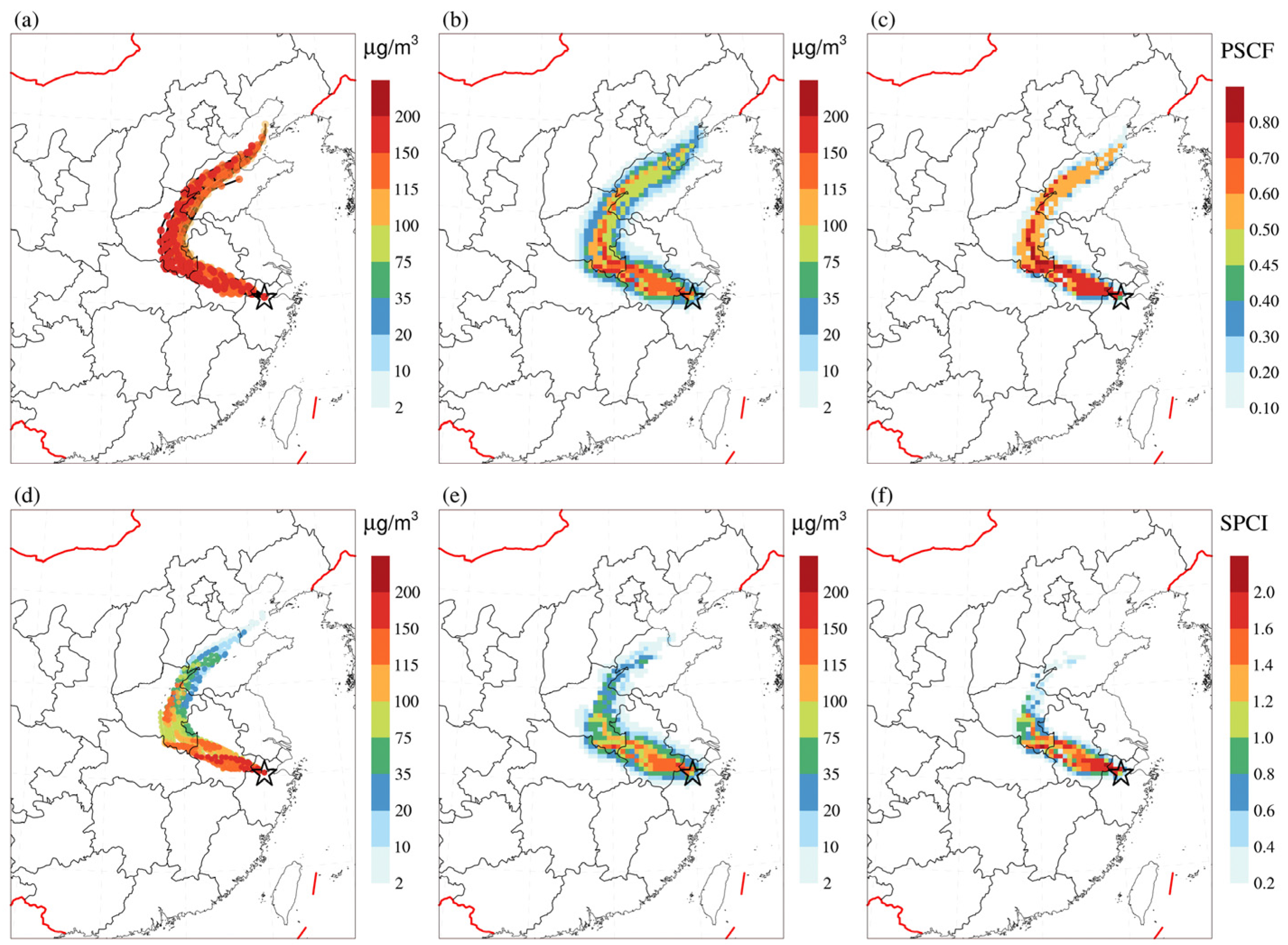
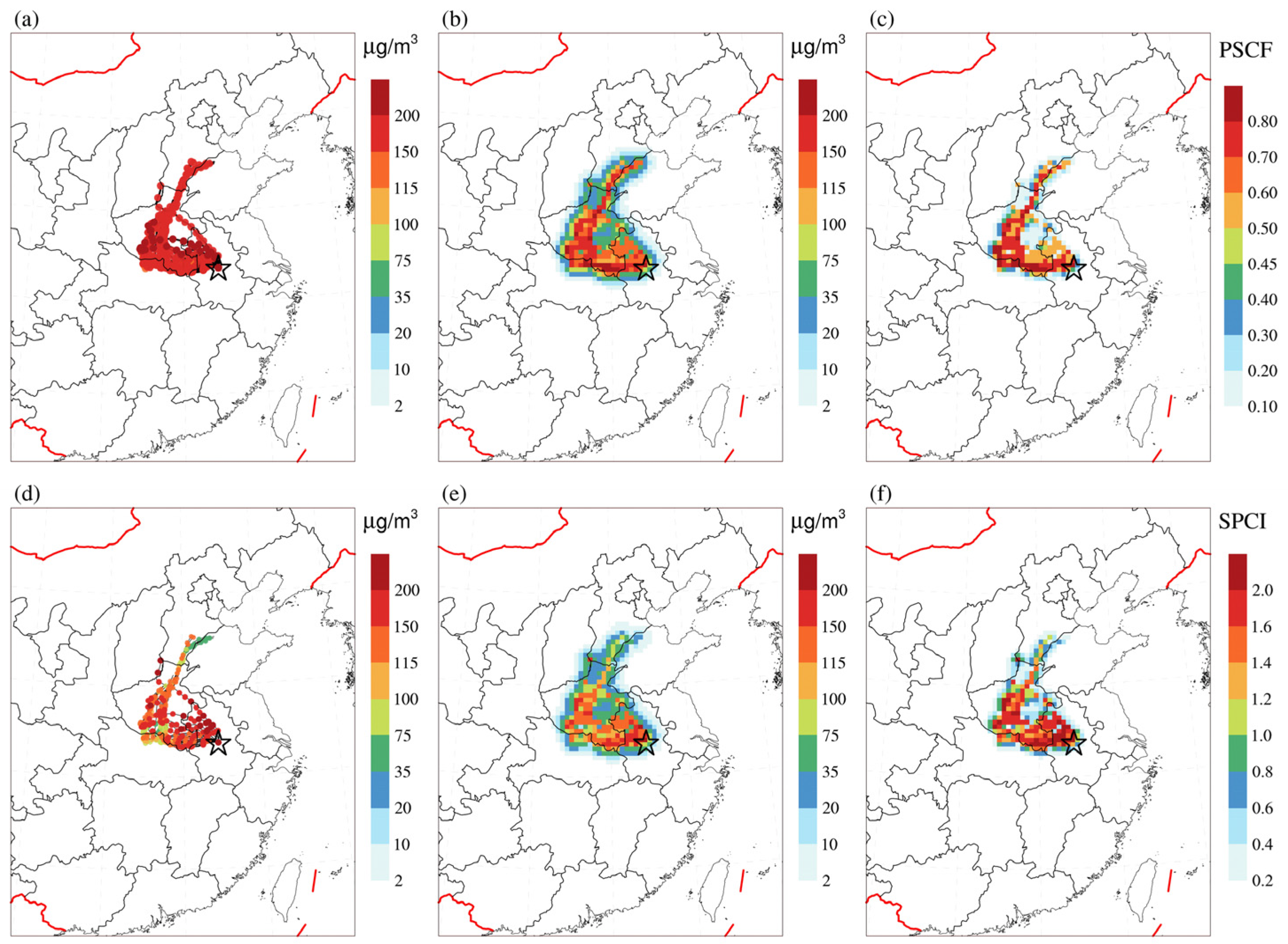
3.2. Identification Potential Sources and Transport Pathway

The potential regional PM_2.5 sources and transport pathways were comparatively analyzed in Hangzhou, Shanghai, Nanjing, and Hefei on 29 January 2020 (Figure 3, Figure 4, Figure 5, Figure 6 and Figure 7). The conventional CWT and PSCF methods were based on PM_2.5 concentrations at receptor sites, where each backward trajectory (Figure 3a, Figure 4a, Figure 5a and Figure 6a) was assigned with the same concentration of receptor for statistical analysis to qualitatively identify potential sources. In contrast, the TCTM utilized the transport flux of backward trajectories, integrating wind fields and spatiotemporal PM_2.5 concentrations to reconstruct the PM_2.5 distributions along backward trajectories (Figure 3d, Figure 4d, Figure 5d and Figure 6d).

There were significant differences in the regional distributions of PM_2.5 concentrations derived from backward trajectories between the two models. Compared to the receptor-assigned trajectory concentrations (Figure 3a, Figure 4a, Figure 5a and Figure 6a), the simulated trajectory concentrations (Figure 3d, Figure 4d, Figure 5d and Figure 6d) more accurately captured reflected the spatiotemporal variations of PM_2.5 along the air-mass trajectories, which was consistent with the PM_2.5 variations in the backward-trajectory channels (Figure 2). Based on the concentration distributions of backward trajectories, we identified and located the major pollution sources affecting the receptor cities. The CWT method calculated trajectory-weighted concentrations (Figure 3b, Figure 4b, Figure 5b and Figure 6b) by weighting the residence time and the assigned trajectory concentrations (Figure 3a, Figure 4a, Figure 5a and Figure 6a). In contrast, the source-receptor WCS method determined the source-region weighted concentrations (Figure 3e, Figure 4e, Figure 5e and Figure 6e) by normalizing the transport decay factors of air masses with the simulated trajectory concentrations (Figure 3d, Figure 4d, Figure 5d and Figure 6d).

The potential sources of high WCS values (>100 µg·m⁻³) in Hangzhou on the 29th were distributed from southeastern Henan to central–southern Anhui and northern Zhejiang along the air trajectory after the wind direction shifted (Figure 3e). Additionally, eastern–central Henan exhibited lower WCS values (<100 µg·m⁻³). The more distant Bohai and Shandong regions had a minimal influence on Hangzhou PM_2.5, consistent with the analysis results in Figure 2b. However, the CWT method identified nearly all regions along the trajectory (>75 µg·m⁻³) as major potential PM_2.5 sources, which differed from the results in Figure 2e. In Shanghai, the potential sources of high WCS values (>100 µg·m⁻³) were primarily distributed in Zhoukou and along the trajectory from Bengbu to Shanghai (Figure 4e). The WCS values were relatively low at the junction between Zhoukou and Anhui, consistent with the analysis results shown in Figure 2b. However, the CWT method revealed that the CWT values in the Shandong and Zhoukou–Fuyang regions were relatively high (>100 µg·m⁻³), identified as important potential sources of PM_2.5. In Nanjing, the high WCS values (>115 µg·m⁻³) primarily distributed from the southern end of BTH to Zhengzhou and from Fuyang to Bengbu along the trajectory (Figure 5e). Additionally, the lower WCS values exhibited in Xuchang were consistent with the analysis in Figure 2d. However, the CWT method revealed that Xuchang had overall higher CWT values (>150 µg·m⁻³), and western Shandong was also identified as a significant PM_2.5 potential source. In Hefei, the potential source areas of high CWS values (>100 µg·m⁻³) were primarily distributed from Zhengzhou to Hefei (Figure 6e). Meanwhile, regions from BTH to Zhengzhou with relatively lower WCS values had a minor impact on Hefei PM_2.5, consistent with the findings in Figure 2e. However, according to the CWT method, the BTH to Zhengzhou regions exhibited generally higher CWT values (>100 µg·m⁻³), identified as major potential source of PM_2.5. Thus, the WCS method not only identified major potential sources but also more accurately reflected the pollution characteristics. Additionally, compared to the CWT method, the WCS method significantly enhanced identification accuracy and better highlighted the key pollution sources.

After identifying major potential sources, pollution transport pathways were analyzed through trajectory concentration distributions. The PSCF values of (Figure 3c, Figure 4c, Figure 5c and Figure 6c) were calculated based on trajectory concentrations (Figure 3a, Figure 4a, Figure 5a, and Figure 6a) associated with receptor sites, with higher values indicating the main potential pollution sources and directions. In the new method, weighted concentrations of source regions (Figure 3e, Figure 4e, Figure 5e and Figure 6e) were calculated using a normalized weighted transport factor derived from the simulated trajectory concentrations (Figure 3d, Figure 4d, Figure 5d and Figure 6d). The ratio of these concentrations to the pollution threshold (PM_2.5 = 75 µg·m⁻³) was defined as the SPCI (Figure 3f, Figure 4f, Figure 5f and Figure 6f), where SPCI > 1 indicated more severe pollution and greater potential influence.

Therefore, in Hangzhou, the main PM_2.5 pollution transport pathways (SPCI > 1) spanned from southeastern Henan to central–southern Anhui and northern Zhejiang (Figure 3f), consistent with the high WCS values (Figure 3e) and high PM_2.5 regions traced by the backward trajectory (Figure 2b). However, all the regions along the trajectories were classified as pollution source regions by PSCF, which differed significantly from the actual simulated PM_2.5 concentrations (Figure 3d) and vertical profile variations (Figure A1). In Shanghai, two transport pathways were identified (Figure 4a,d). The primary pollution transport route (SPCI > 1) extended from central–eastern Henan via Nanjing to Shanghai (Figure 4f), matching high WCS values (Figure 4e) and PM_2.5 levels (Figure 2e). Conversely, the coastal pathway (Shandong–Jiangsu–Shanghai) was erroneously identified as a pollution channel by PSCF, contradicting PM_2.5 distribution (Figure 4d) and backward-trajectory analysis (Figure A2). In Nanjing, the polluted pathway (SPCI > 1) was located along BTH–Zhengzhou–Bengbu–Nanjing (Figure 5f), aligning with high WCS values (Figure 5e) and the PM_2.5 concentrations (Figure 2d) traced by the backward trajectory. However, both pathways were classified as pollution transport channels by the PSCF method, which deviated from the actual results (Figure A3). Additionally, the boundaries between southern BTH and Shandong were not clearly distinguished. In Hefei, the primary PM_2.5 pollution transport route (SPCI > 1) originated from central Henan to southern Henan and Hefei (Figure 6f), consistent with the distributions of high WCS values (Figure 6e) and the PM_2.5 high-value regions (Figure 2e) traced by backward trajectory. Moreover, the SPCI outperformed PSCF in pinpointing pollution sources in the northwestern Hefei and its surrounding areas, corroborated by trajectory analysis (Figure 6d and Figure A4). Overall, compared to PSCF (Figure 3c, Figure 4c, Figure 5c and Figure 6c), the SPCI (Figure 3f, Figure 4f, Figure 5f and Figure 6f) more precisely identified PM_2.5 sources and key pollution transport distance within the channel.

In summary, the traditional PSCF and CWT methods merely qualitatively identified the potential PM_2.5 sources in Hangzhou, Shanghai, Nanjing, and Hefei, without differentiating key potential sources or critical transport distances. In contrast, the TCTM, by thoroughly analyzing the spatiotemporal distribution of PM_2.5 concentrations and establishing source–receptor relationships, enabled a more precise identification and localization of pollution sources, as well as a clear distinction of key pollution distances along transport pathways. The key pollution transport pathways were identified as follows: Hangzhou: southern Henan–Tongling–Hangzhou; Shanghai: Fuyang–Nanjing–Shanghai; Nanjing: BTH–Zhengzhou–Xuchang–Bengbu–Nanjing; and Hefei: Zhengzhou–Nanyang–Hefei.

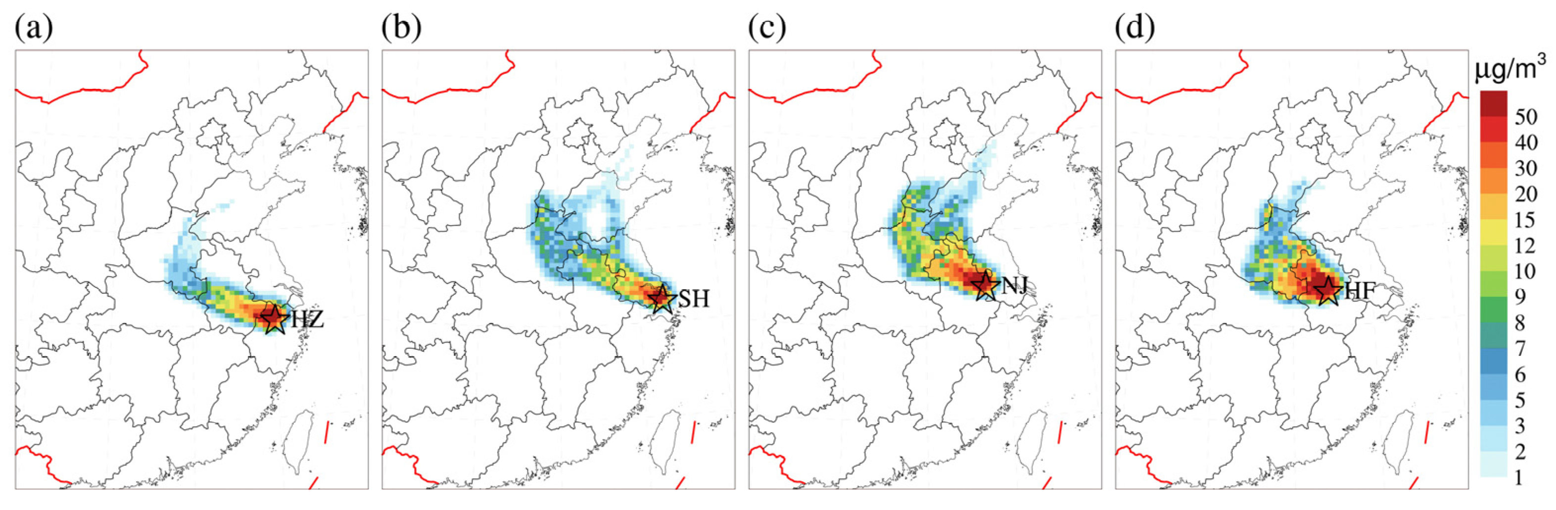
3.3. Regional Transport Contribution

After identifying and analyzing the primary PM_2.5 sources and key transport pathways, we applied the TCTM to quantify the contribution of regional transport to receptor PM_2.5 concentrations in Hangzhou, Shanghai, Nanjing, and Hefei on 29 January 2020 (Figure 7). This approach constitutes a significant innovation and key advantage of this study.

In Hangzhou, the primary PM_2.5 source regions were located from southern Anhui to the vicinity of Hangzhou (Figure 7a), consistent with the major potential sources (Figure 3e) and the high PM_2.5 regions identified through backward-trajectory tracking, with an average contribution over 12 µg·m⁻³. Additionally, the region from the southeastern corner of Henan to Hefei was also identified as a significant contributor. The spatial distribution of the primary affecting Hangzhou aligns with the pollution pathway analysis results (Figure 3f). In Shanghai, the primary PM_2.5 source regions were predominantly distributed along the Nanjing–southeast Jiangsu corridor (Figure 7b), aligned with the key potential sources (Figure 4e) and the high PM_2.5 regions along pollution backward trajectories (Figure 2c). The average PM_2.5 contribution from Changzhou, Wuxi, and Suzhou exceeded 20 µg·m⁻³. In contrast, contributions from Hebei, Shandong, and Henan were relatively small (Figure A2), which can be attributed to both the lower regional PM_2.5 concentrations and non-main source regions. In Nanjing, the primary PM_2.5 source regions were located in northern Anhui and the northwestern area of Nanjing (Figure 7c), particularly along the Fuyang–Bengbu–Nanjing line. This spatial pattern aligned closely with the distribution of major potential sources (Figure 5e) and the high PM_2.5 regions along polluted backward trajectories (Figure 2d), with an average contribution over 20 µg·m⁻³ from these regions. In addition, the border regions of Hebei, Shanxi, and Henan also contributed significantly to the PM_2.5 level in Nanjing (10~15 µg·m⁻³), consistent with the high-value PM_2.5 areas along the pollution pathway (Figure A3). In Hefei, the primary PM_2.5 source regions were located along the border between southeastern Henan and Anhui, as well as in the northwestern sector of Hefei (Figure 7d). These regions aligned with the key potential sources (Figure 6e) and the high PM_2.5 concentration zones traced by the backward trajectory (Figure 2e). The average PM_2.5 contribution from local surrounding areas exceeded 40 µg·m⁻³, while that in southeastern Henan and northwestern Anhui ranged between 15~40 µg·m⁻³. The findings regarding the primary PM_2.5 sources were also consistent with the spatial analysis of high PM_2.5 areas along transport pathway (Figure 6f).

In summary, the TCTM enabled a quantitative estimation of regional PM_2.5 transport contributions to four receptor cities (Hangzhou, Shanghai, Nanjing, and Hefei). Furthermore, the spatial distribution of major contributing regions aligned with both the identified potential sources and the high PM_2.5 concentration areas through backward-trajectory tracking. The results also demonstrated that the TCTM can accurately identify and locate primary potential pollution sources, determine key pollutant transport pathways, and further validate the rationality and validity of the potential-source identification methodology.

4. Conclusions

In this study, we proposed a Trajectory-Channel Transport Model (TCTM) that integrated source–receptor relationships, enhancing the accurate identification of potential sources and enabling quantitative impact assessment.

By simulating PM_2.5 concentrations in four major cities (Hangzhou, Shanghai, Nanjing, and Hefei) on 29 January 2020, and tracking backward-trajectory analysis, primary potential sources, and transport pathways, the results demonstrated that the CWS method realistically reflected the PM_2.5 pollution characteristics of source regions and accurately located the key potential sources. Additionally, the SPCI method further judged critical pollution transport pathways. In all four cities, both the WCS and SPCI enhanced the precision of PM_2.5 source identification, effectively distinguishing key sources and clarifying the distance ranges of major PM_2.5 pollution pathway. More importantly, the TCTM quantified regional PM_2.5 transport contributions.

Thus, the TCTM proved to be feasible, more reliable and reasonable for potential source analysis, enabling the accurate identification, location, and differentiation of key sources. Furthermore, the TCTM can quickly and accurately identify the critical transport pathways, providing an efficient and robust analytical tool for regional air-quality management and pollution control strategies.

References

1. Cheng, Z.; Luo, L.N.; Wang, S.X.; Wang, Y.G.; Sharma, S.; Shimadera, H.; Wang, X.L.; Bress, M.; de Miranda, R.M.; Jiang, J.K.; et al. Status and characteristics of ambient PM2.5 pollution in global megacities. Environ. Int. 2016, 89–90, 212–221. [Google Scholar] [CrossRef] [PubMed]
2. Shen, L.J.; Zhao, T.L.; Liu, J.N.; Wang, H.L.; Bai, Y.Q.; Kong, S.F.; Shu, Z.Z. Regional transport patterns for heavy PM2.5 pollution driven by strong cold airflows in Twain-Hu Basin, Central China. Atmos. Environ. 2022, 269, 118847. [Google Scholar] [CrossRef]
3. Tao, T.H.; Shi, Y.S.; Gilbert, K.M.; Liu, X.Y. Spatiotemporal variations of air pollutants based on ground observation and emission sources over 19 Chinese urban agglomerations during 2015–2019. Sci. Rep. 2022, 12, 4293. [Google Scholar] [CrossRef] [PubMed]
4. Cohen, A.J.; Brauer, M.; Burnett, R.; Anderson, H.R.; Frostad, J.; Estep, K.; Balakrishnan, K.; Brunekreef, B.; Dandona, L.; Dandona, R.; et al. Estimates and 25-year trends of the global burden of disease attributable to ambient air pollution: An analysis of data from the Global Burden of Diseases Study 2015. Lancet 2017, 389, 1907–1918. [Google Scholar] [CrossRef] [PubMed]
5. Smolker, H.R.; Reid, C.E.; Friedman, N.P.; Banich, M.T. The Association between Exposure to Fine Particulate Air Pollution and the Trajectory of Internalizing and Externalizing Behaviors during Late Childhood and Early Adolescence: Evidence from the Adolescent Brain Cognitive Development (ABCD) Study. Environ. Health Persp. 2024, 132, 87001. [Google Scholar] [CrossRef] [PubMed]
6. Rai, P.K. Impacts of particulate matter pollution on plants: Implications for environmental biomonitoring. Ecotox. Environ. Safe 2016, 129, 120–136. [Google Scholar] [CrossRef] [PubMed]
7. Huang, R.J.; Zhang, Y.L.; Bozzetti, C.; Ho, K.F.; Cao, J.J.; Han, Y.M.; Daellenbach, K.R.; Slowik, J.G.; Platt, S.M.; Canonaco, F.; et al. High secondary aerosol contribution to particulate pollution during haze events in China. Nature 2014, 514, 218–222. [Google Scholar] [CrossRef] [PubMed]
8. Li, J.; Du, H.Y.; Wang, Z.F.; Sun, Y.L.; Yang, W.Y.; Li, J.J.; Tang, X.; Fu, P.Q. Rapid formation of a severe regional winter haze episode over a mega-city cluster on the North China Plain. Environ. Pollut. 2017, 223, 605–615. [Google Scholar] [CrossRef] [PubMed]
9. Zhou, W.Q.; Yu, W.J.; Qian, Y.G.; Han, L.J.; Pickett, S.T.A.; Wang, J.; Li, W.F.; Ouyang, Z.Y. Beyond city expansion: Multi-scale environmental impacts of urban megaregion formation in China. Natl. Sci. Rev. 2021, 9, nwab107. [Google Scholar] [CrossRef] [PubMed]
10. Guo, D.P.; Wang, R.; Zhao, P. Spatial distribution and source contributions of PM2.5 concentrations in Jincheng, China. Atmos. Pollut. Res. 2020, 11, 1281–1289. [Google Scholar] [CrossRef]
11. Yang, X.C.; Wu, Q.Z.; Zhao, R.; Cheng, H.Q.; He, H.J.; Ma, Q.; Wang, L.N.; Luo, H. New method for evaluating winter air quality: PM2.5 assessment using Community Multi-Scale Air Quality Modeling (CMAQ) in Xi’an. Atmos. Environ. 2019, 211, 18–28. [Google Scholar] [CrossRef]
12. Yang, X.C.; Xiao, H.; Wu, Q.Z.; Wang, L.N.; Guo, Q.Y.; Cheng, H.Q.; Wang, R.R.; Tang, Z.Y. Numerical study of air pollution over a typical basin topography: Source appointment of fine particulate matter during one severe haze in the megacity Xi’an. Sci. Total Environ. 2020, 708, 135213. [Google Scholar] [CrossRef] [PubMed]
13. Zhang, Y.L.; Zhu, B.; Gao, J.H.; Kang, H.Q.; Yang, P.; Wang, L.L.; Zhang, J.K. The source apportionment of primary PM2.5 in an aerosol pollution event over Beijing-Tianjin-Hebei Region using WRF-Chem, China. Aerosol Air Qual. Res. 2017, 17, 2966–2980. [Google Scholar] [CrossRef]
14. Ming, L.L.; Jin, L.; Li, J.; Fu, P.Q.; Yang, W.Y.; Liu, D.; Zhang, G.; Wang, Z.F.; Li, X.D. PM2.5 in the Yangtze River Delta, China: Chemical compositions, seasonal variations, and regional pollution events. Environ. Pollut. 2017, 223, 200–212. [Google Scholar] [CrossRef] [PubMed]
15. Chang, X.; Wang, S.X.; Zhao, B.; Xing, J.; Liu, X.X.; Wei, L.; Song, Y.; Wu, W.J.; Cai, S.Y.; Zheng, H.T.; et al. Contributions of inter-city and regional transport to PM2.5 concentrations in the Beijing-Tianjin-Hebei region and its implications on regional joint air pollution control. Sci. Total Environ. 2019, 660, 1191–1200. [Google Scholar] [CrossRef] [PubMed]
16. Huang, S.; Tang, X.; Xu, W.S.; Wang, Z.; Cheng, H.S.; Li, J.; Wu, Q.Z.; Wang, Z.F. Application of ensemble forecast and linear regression method in improving PM10 forecast over Beijing areas. Acta Sci. Circumst. 2015, 35, 56–64. [Google Scholar]
17. Tian, J.Y.; Hopke, P.K.; Cai, T.Q.; Fan, Z.J.; Yu, Y.; Zhao, K.N.; Zhang, Y.X. Evaluation of impact of “2 + 26′′ regional strategies on air quality improvement of different functional districts in Beijing based on a long-term field campaign. Environ. Res. 2022, 212, 113452. [Google Scholar] [CrossRef] [PubMed]
18. Yang, T.; Wang, Z.F.; Zhang, B.; Wang, X.Q.; Wang, W.; Gbauidi, A.; Gong, Y.B. Evaluation of the effect of air pollution control during the Beijing 2008 Olympic Games using Lidar data. Chin. Sci. Bull. 2010, 55, 1311–1316. [Google Scholar] [CrossRef]
19. Zhang, S.J.; Wu, Y.; Huang, R.K.; Wang, J.D.; Yan, H.; Zheng, Y.L.; Hao, J.M. High-resolution simulation of link-level vehicle emissions and concentrations for air pollutants in a traffic-populated eastern Asian city. Atmos. Chem. Phys. 2016, 16, 9965–9981. [Google Scholar] [CrossRef]
20. Cheng, J.; Su, J.P.; Cui, T.; Li, X.; Dong, X.; Sun, F.; Yang, Y.Y.; Tong, D.; Zheng, Y.X.; Li, Y.S.; et al. Dominant role of emission reduction in PM2.5 air quality improvement in Beijing during 2013–2017, a model-based decomposition analysis. Atmos. Chem. Phys. 2019, 19, 6125–6146. [Google Scholar] [CrossRef]
21. Wang, H.; Liu, Q.; Wang, Y.; Li, Y.; Zhang, D.D.; Zhu, Y.J.; Hong, P.P. Numerical study of PM2.5 pollution in Taizhou based on Model-3/CMAQ and CAMx. Environ. Sustainable Dev. 2019, 44, 93–96. [Google Scholar]
22. Liu, C.; Huang, J.P.; Hu, X.M.; Hu, C.; Wang, Y.W.; Fang, X.Z.; Luo, L.; Xiao, H.W.; Xiao, H.Y. Evaluation of WRF-Chem simulations on vertical profiles of PM2.5 with UAV observations during a haze pollution event. Atmos. Environ. 2021, 252, 118332. [Google Scholar] [CrossRef]
23. Hu, W.Y.; Zhao, T.L.; Bai, Y.Q.; Kong, S.F.; Xiong, J.; Sun, X.Y.; Yang, Q.J.; Gu, Y.; Lu, H.C. Importance of regional PM2.5 transport and precipitation washout in heavy air pollution in the Twain-Hu Basin over Central China: Observational analysis and WRF-Chem simulation. Sci. Total Environ. 2021, 758, 143710. [Google Scholar] [CrossRef] [PubMed]
24. Wang, T.; Li, J.; Wang, W.; Yang, W.Y.; Hao, J.Q.; Du, H.Y. Numerical simulation study on source apportionment of PM2.5 in a heavy winter pollution event over Beijing area. Acta Sci. Circumst. 2019, 39, 1025–1038. [Google Scholar]
25. Liu, Y.; Zheng, M.; Yu, M.Y.; Cai, X.H.; Du, H.Y.; Li, J.; Zhou, T.; Yan, C.Q.; Wang, X.S.; Shi, Z.B.; et al. High-time-resolution source apportionment of PM2.5 in Beijing with multiple models. Atmos. Chem. Phys. 2019, 19, 6595–6609. [Google Scholar] [CrossRef]
26. Ying, Q.; Lu, J.; Allen, P.; Livingstone, P.; Kaduwela, A.; Kleeman, M. Modeling air quality during the California Regional PM10/PM2.5 Air Quality Study (CRPAQS) using the UCD/CIT source-oriented air quality model-Part I. Base case model result. Atmos. Environ. 2008, 42, 8954–8966. [Google Scholar] [CrossRef]
27. Lin, X.; Tong, J.L.; Wang, Y.F.; Chen, Y.X.; Liu, Y.L.; Zhang, X.; Ao, C.J.; Liu, H.T. Analysis of Causes and Sources of Summer Ozone Pollution in Rizhao Based on CMAQ and HYSPLIT Models. Envrion. Sci. 2023, 44, 3098–3107. [Google Scholar]
28. Wu, J.B.; Wang, Z.F.; Wang, Q.; Li, J.; Xu, J.M.; Chen, H.S.; Ge, B.Z.; Zhou, G.Q.; Chang, L.Y. Development of an on-line source-tagged model for sulfate, nitrate and ammonium: A modeling study for highly polluted periods in Shanghai, China. Environ. Pollut. 2017, 221, 168–179. [Google Scholar] [CrossRef] [PubMed]
29. Tuan, V.V.; Juana, M.D.; Roy, M.H. Review: Particle number size distributions from seven major sources and implications for source apportionment studies. Atmos. Environ. 2015, 112, 114–132. [Google Scholar]
30. Wang, Z.S.; Chien, C.J.; Tonnesen, G.S. Development of a tagged species source apportionment algorithm to characterize three-dimensional transport and transformation of precursors and secondary pollutants. J. Geophys. Res. 2009, 114, D21206. [Google Scholar] [CrossRef]
31. Gao, Z.Q.; Zhou, X.H. A review of the CAMx, CMAQ, WRF-Chem and NAQPMS models: Application, evaluation and uncertainty factors. Environ. Pollut. 2024, 343, 123183. [Google Scholar] [CrossRef] [PubMed]
32. Wang, F.; Chen, D.S.; Cheng, S.Y.; Li, J.B.; Li, M.J.; Ren, Z.H. Identification of regional atmospheric PM10 transport pathways using HYSPLIT, MM5-CMAQ and synoptic pressure pattern analysis. Environ. Model. Softw. 2010, 25, 927–934. [Google Scholar] [CrossRef]
33. Shikhovtsev, M.Y.; Molozhnikova, Y.V.; Obolkin, V.A.; Potemkin, V.L.; Lutskin, E.S.; Khodzher, T.V. Features of Temporal Variability of the Concentrations of Gaseous Trace Pollutants in the Air of the Urban and Rural Areas in the Southern Baikal Region (East Siberia, Russia). Appl. Sci. 2024, 14, 8327. [Google Scholar] [CrossRef]
34. Li, D.P.; Liu, J.G.; Zhang, J.S.; Gui, H.Q.; Du, P.; Yu, T.Z.; Wang, J.; Lu, Y.H.; Liu, W.Q.; Cheng, Y. Identification of long-range transport pathways and potential sources of PM2.5 and PM10 in Beijing from 2014 to 2015. J. Environ. Sci. 2017, 56, 214–229. [Google Scholar] [CrossRef] [PubMed]
35. Wang, W.F.; Yu, J.; Cui, Y.; He, J.; Xue, P.; Cao, W.; Ying, H.M.; Gao, W.K.; Yan, Y.C.; Hu, B.; et al. Characteristics of fine particulate matter and its sources in an industrialized coastal city, Ningbo, Yangtze River Delta, China. Atmos. Res. 2018, 203, 105–117. [Google Scholar] [CrossRef]
36. Brereton, C.A.; Johnson, M.R. Identifying sources of fugitive emissions in industrial facilities using trajectory statistical methods. Atmos. Environ. 2012, 51, 46–55. [Google Scholar] [CrossRef]
37. Wang, M.; Duan, Y.S.; Xu, W.; Wang, Q.Y.; Zhang, Z.Z.; Yuan, Q.; Li, X.W.; Han, S.W.; Tong, H.J.; Huo, J.T.; et al. Measurement report: Characterisation and sources of the secondary organic carbon in a Chinese megacity over 5 years from 2016 to 2020. Atmos. Chem. Phys. 2022, 22, 12789–12802. [Google Scholar] [CrossRef]
38. Karaca, F.; Anil, I.; Alagha, O. Long-range potential source contributions of episodic aerosol events to PM10 profile of a megacity. Atmos. Environ. 2009, 43, 5713–5722. [Google Scholar] [CrossRef]
39. Pu, X.; Li, Z.L.; Cao, Y.Q.; Jiang, C.T.; Zhang, Y.; Gao, Y.H.; Zhang, W.D.; Zhai, C.Z. Transport pathways and potential source contribution of PM2.5 pollution in Chongqing from 2015 to 2020. Acta Sci. Circumst. 2022, 42, 49–59. [Google Scholar]
40. Wang, A.P.; Zhu, B.; Yin, Y.; Jin, L.J.; Zhang, L. Aerosol number concentration properties and potential sources areas transporting to the top of mountain Huangshan in summer. China Environ. Sci. 2014, 34, 852–861. [Google Scholar]
41. Lei, Y.; Zhang, X.L.; Kang, P.; Wang, H.L.; Qing, Q.; Ou, Y.H.; Lu, N.S.; Deng, Z.C. Analysis of Transport Pathways and Potential Sources of Atmospheric Particulate Matter in Zigong, in South of Sichuan Province. Envrion. Sci. 2020, 41, 3021–3030. [Google Scholar]
42. Seinfeld, J.H.; Pandis, S.N.; Noone, K. Atmospheric Chemistry and Physics: From Air Pollution to Climate Change. Phys. Today 1998, 51, 88–90. [Google Scholar] [CrossRef]
43. Hsu, Y.K.; Holsen, T.M.; Hopke, P.K. Comparison of hybrid receptor models to locate PCB sources in Chicago. Atmos. Envirion. 2003, 37, 545–562. [Google Scholar] [CrossRef]
44. Cheng, I.; Zhang, L.; Blanchard, P.; Dalziel, J.; Tordon, R. Concentration-weighted trajectory approach to identifying potential sources of speciated atmospheric mercury at an urban coastal site in Nova Scotia, Canada. Atmos. Chem. Phys. 2013, 13, 6031–6048. [Google Scholar] [CrossRef]
45. Zhang, Y.P.; Chen, J.; Yang, H.N.; Li, R.J.; Yu, Q. Seasonal variation and potential source regions of PM2.5-bound PAHs in the megacity Beijing, China: Impact of regional transport. Environ. Pollut. 2017, 231, 329–338. [Google Scholar] [CrossRef] [PubMed]
46. Wang, Z.F.; Li, J.; Wang, Z.; Yang, W.Y.; Tang, X.; Ge, B.Z.; Yan, P.Z.; Zhu, L.L.; Chen, X.S.; Chen, H.S.; et al. Modeling study of regional severe hazes over mid-eastern China in January 2013 and its implications on pollution prevention and control. Sci. China Earth Sci. 2014, 57, 3–13. [Google Scholar] [CrossRef]
47. Wang, Z.F.; Xie, F.Y.; Wang, X.Q.; An, J.L.; Zhu, J. Development and Application of Nested Air Quality Prediction Modeling System. Chinese J. Atmos. Sci. 2006, 30, 778–790. [Google Scholar]
48. Wang, W.D.; Chen, H.S.; Wu, Q.Z.; Wei, L.F.; Wang, Z.F.; Li, C.; Chen, D.H.; Jiang, Z.M.; Wu, W.W. Numerical study of PM2.5 regional transport over Pearl River Delta during a winter heavy haze event. Acta Sci. Circumst. 2016, 36, 2741–2751. [Google Scholar]
49. Li, J.; Wang, Z.; Zhuang, G.; Luo, G.; Sun, Y.; Wang, Q. Mixing of Asian mineral dust with anthropogenic pollutants over East Asia: A model case study of a super-dust storm in March 2010. Atmos. Chem. Phys. 2012, 12, 7591–7607. [Google Scholar] [CrossRef]
50. Li, J.; Wang, Z.F.; Wang, X.; Yamaji, K.; Takigawa, M.; Kanaya, Y.; Pochanart, P.; Liu, Y.; Irie, H.; Hu, B.; et al. Impacts of aerosols on summertime tropospheric photolysis frequencies and photochemistry over Central Eastern China. Atmos. Envirion. 2011, 45, 1817–1829. [Google Scholar] [CrossRef]
51. Zaveri, R.A.; Peters, L.K. A new lumped structure photochemical mechanism for large-scale applications. J. Geophys. Res. 1999, 104, 30387–30415. [Google Scholar] [CrossRef]
52. Nenes, A.; Pandis, S.N.; Pilinis, C. ISORROPIA: A New Thermodynamic Equilibrium Model for Multiphase Multicomponent Inorganic Aerosols. Aquatic Geochem. 1998, 4, 123–152. [Google Scholar] [CrossRef]
53. Odum, J.R.; Jungkamp, T.P.W.; Griffin, R.J.; Flagan, R.C.; Seinfeld, J.H. The Atmospheric Aerosol-Forming Potential of Whole Gasoline Vapor. Science 1997, 276, 96–97. [Google Scholar] [CrossRef] [PubMed]
54. Luo, G.; Wang, Z.F. A global environmental atmospheric transport model (GEATM): Model description and validation. Chin. J. Atmos. Sci. 2006, 30, 504–518. [Google Scholar]
55. Athanasopoulou, E.; Tombrou, M.; Pandis, S.N.; Russell, A.G. The role of sea-salt emissions and heterogeneous chemistry in the air quality of polluted coastal areas. Atmos. Chem. Phys. 2008, 8, 5755–5769. [Google Scholar] [CrossRef]
56. Yang, T.; Gbaguidi, A.; Yan, P.Z.; Zhang, W.D.; Zhu, L.L.; Yao, X.F.; Wang, Z.F.; Chen, H. Model elucidating the sources and formation mechanisms of severe haze pollution over Northeast mega-city cluster in China. Environ. Pollut. 2017, 230, 692–700. [Google Scholar] [CrossRef] [PubMed]
57. Pan, Y.; Zheng, J.; Xiao, H. Simulation Evaluation of the Contribution of Typical PM2.5 Pollution and Trans-regional Transport to Ningbo Pollution in the Yangtze River Delta. Environ. Sci. 2023, 44, 634–645. [Google Scholar]
58. Seibert, P.; Kromp-Kolb, H.; Baltensperger, U.; Jost, D.T.; Schwikowski, M. Trajectory Analysis of High-Alpine Air Pollution Data. Air Pollut. Model. Its Appl. X 1994, 18, 595–596. [Google Scholar]
59. Li, R.; Li, Q.; Xu, J.; Li, L.; Ge, C.J.; Huang, L.; Sun, D.H.; Liu, Z.Y.; Zhang, K.; Zhou, G.Z.; et al. Regional Air Pollution Process in Winter over the Yangtze River Delta and Its Influence on Typical Northern Cities. Envrion. Sci. 2020, 41, 1520–1534. [Google Scholar]
60. Yan, S.M.; Wang, Y.; Guo, W.; Li, Y.; Zhang, F.S. Characteristics, Transportation, Pathways, and Potential Sources of Air Pollution During Autumn and Winter in Taiyuan. Envrion. Sci. 2019, 40, 4801–4809. [Google Scholar]
61. Pan, Y.; Zheng, Z.; Fang, F.X.; Liang, F.H.; Tong, L.; Xiao, H. A Comprehensive Study on Winter PM2.5 Variation in the Yangtze River Delta: Unveiling Causes and Pollution Transport Pathways. Atmosphere 2024, 15, 1037. [Google Scholar] [CrossRef]
Figure 1. A schematic of the air-mass trajectory transport channel. The blue dotted line indicates trajectory k, LP denotes the source grid (i,j), the P0 denotes the receptor site; Cijk, Vijk, τijk, and Mijk represent the PM2.5 concentration, wind speed, residence time, and total transported masses at grid cell (i,j) along trajectory k, respectively. dx, dy, and dz are the spatial resolution of grid cell (i,j), while L and TLP denote the distance and transport time between LP to P0, respectively.
Atmosphere 16 00883 g001
Figure 2. (a) The spatial distribution of daily mean PM2.5 concentration, the blue, green, black and purple clustered trajectories represent the air-mass transport pathways for Hangzhou (HZ), Shanghai (SH), Nanjing (NJ), and Hefei (HF), respectively. Points marked along each trajectory indicate the corresponding backward hour. (be) show the vertical PM2.5 concentration distributions along the clustered trajectory of HZ, SH, NJ, and HF, respectively.
Atmosphere 16 00883 g002
Figure 3. The identification and location of PM2.5 potential sources and pollution transport pathways in Hangzhou. (a) PM2.5 trajectory concentrations derived from receptor site; (b) the CWT values; (c) the PSCF values; (d) simulated PM2.5 trajectory concentrations; (e) the WCS values; and (f) the SPCI values. The star represents the Hangzhou location.
Atmosphere 16 00883 g003
Figure 4. The identification and location of PM2.5 potential sources and pollution transport pathways in Shanghai. (a) PM2.5 trajectory concentrations derived from receptor site; (b) the CWT values; (c) the PSCF values; (d) simulated PM2.5 trajectory concentrations; (e) the WCS values; and (f) the SPCI values. In (a,d), the two blue clustering trajectories represent the inland and coastal channels. The star represents the Shanghai location.
Atmosphere 16 00883 g004
Figure 5. The identification and location of PM2.5 potential sources and pollution transport pathways in Nanjing. (a) PM2.5 trajectory concentrations derived from receptor site; (b) the CWT values; (c) the PSCF values; (d) simulated PM2.5 trajectory concentrations; (e) the WCS values; and (f) the SPCI values. In (a,d), the two blue clustering trajectories represent the two different channels. The star represents the Nanjing location.
Atmosphere 16 00883 g005
Figure 6. The identification and location of PM2.5 potential sources and pollution transport pathways in Hefei. (a) PM2.5 trajectory concentrations derived from receptor site; (b) the CWT values; (c) the PSCF values; (d) simulated PM2.5 trajectory concentrations; (e) the WCS values; and (f) the SPCI values. The star represents the Hefei location.
Atmosphere 16 00883 g006
Figure 7. An assessment of regional PM2.5 transport contribution to Hangzhou (a), Shanghai (b), Nanjing (c), and Hefei (d), respectively. The black star denotes the location of the receptor city.
Atmosphere 16 00883 g007
Disclaimer/Publisher’s Note: The statements, opinions and data contained in all publications are solely those of the individual author(s) and contributor(s) and not of MDPI and/or the editor(s). MDPI and/or the editor(s) disclaim responsibility for any injury to people or property resulting from any ideas, methods, instructions or products referred to in the content.