Abstract
The urban heat island (UHI) effect significantly impacts urban environments, particularly along roads, a phenomenon known as urban linear heat (UHIULI). Numerous factors contribute to roads influencing the UHIULI; however, effective mitigation strategies remain a challenge. This study examines the relationship between canopy cover percentage, normalized difference vegetation index, land use types, and three road typologies (local, regional, and state) with land surface temperature. This study is based on data from the city of Adelaide, Australia, using spatial analysis, and statistical modelling. The results reveal strong negative correlations between land surface temperature and both canopy cover percentage and normalized difference vegetation index. Additionally, land surface temperature tends to increase with road width. Among land use types, land surface temperature varies from highest to lowest in the order of parkland, industrial, residential, educational, medical, and commercial areas. Notably, the combined influence of the road typology and land use produces varying effects on land surface temperature. Canopy cover percentage and normalized difference vegetation index consistently serve as dominant cooling factors. The results highlight a complex interplay between built and natural environments, emphasizing the need for multi-factor analyses and a framework based on the local climate and the type of roads (local, regional, and state) to effectively evaluate UHIULI mitigation approaches.
1. Introduction
The urban heat island (UHI) effect is a well-documented phenomenon impacting cities [] and its effects can be exacerbated along urban linear infrastructure (ULI). Urban linear heat (UHIULI) [] is the term used to describe the UHI effect along transportation corridors and pipeline networks. Collectively, the UHI impacts across boundary, canyon, surface, and subsurface layers [] and multiple studies have reported increasing tree canopy can provide a cooling benefit via shading and evapotranspiration [,,]. ULI comprises a significant proportion of the land use of cities, with roads alone occupying up to one-third of the urban area []. The area that roads occupy is increasing as cities expand and densify which is also influenced by rising car ownership and use [,]. The corollary of the increase in road area is a decrease in urban green spaces, where roads and driveways expand into the vegetated spaces, such as nature strips and gardens [,,]. These dark and impervious materials used for road construction prevent water infiltration, increase the absorption of solar radiation and trap heat [,,]. This creates a positive heat feedback loop that magnifies the energy budget of cities [], driving the UHIULI [].
A variety of factors determine how UHIULI forms along roads, particularly the width of road (road typology), materials and colours [,,]. Wider roads receive more solar radiation and thus gaining more heat than narrower (often local) roads. Wide roads (such as regional and state highways) typically accommodate more cars and thus are associated with higher anthropogenic heat emissions from vehicles [,,,,,,]. Mitigating heat along roadways has proven to be a challenging task [], with various approaches turning to applying high-albedo and permeable materials, greening adjacent land uses and seeking different designs (morphology-related strategies) to lessen heat and radiation gains [,,,].
The most recommended approach to mitigate UHIULI is to integrate tree canopy cover along roads [,,]. Canopy trees have been reported to provide a cooling benefit of between 1 °C and 30 °C [,]. The effectiveness of canopy tree cooling is influenced by a number of factors including the geometry of crown and leaves, type of tree, density of leaves, connectivity or clustering of tree, and watering schedule [,,,,,,,,,,,,,]. Effectiveness of cooling is also influenced by the width of the road. This creates a physical limitation of the canopy trees in offering shade across the width of the road surface through reducing the sky view factor (SVF). A wider road has an increased SVF, which means more of the sky is visible from a specific point at ground level and potentially allowing for greater solar radiation to reach the road surface [,,,]. In addition, the density of leaves and the percentage of canopy cover of a given area can also reduce wind flow, ventilation, and humidity levels [,,,,,]. The literature identifies various factors that may influence the UHI as a result of road networks, as listed in Table 1 [].
The canopy cover percentage (CCP) is a significant variable influencing UHIULI mitigation along roads [,,,]. CCP represents the proportion of ground area covered by the vertical projection of tree crowns onto the ground, expressed as a percentage. This has led to some agencies introducing policies to achieve a minimum CCP along roads (trees on the sides with their crowns extending over the lanes) []. However, the relationship between the cooling effect of CCP and road width is complicated and often overlooked. Road width can be conceptualized by the number of trafficable lanes []. From a UHIULI mitigation perspective, roads can be divided into three categories: local, regional, and state roads []. This roughly equates to two lanes for local roads, four lanes for regional roads, and six lanes or more for state roads []. The cooling effects of canopy trees linked to the CCP across this three road categorization forms the basis for the inquiry of this paper. Within this framework, three research questions are examined:
- 1.
- How does the UHIULI change with respect to the road hierarchy in relation to variations in CCP?
- 2.
- Is there any optimum value for CCP to obtain the most efficient cooling effect with respect to the road hierarchy?
- 3.
- To what extent do other factors beyond canopy cover (Table 1: NDVI, land use type, geographic coordinates and elevation) contribute to UHIULI mitigation (LST) relative to the road hierarchy?

Table 1.
Contributing factors to UHIULI in this study.
Table 1.
Contributing factors to UHIULI in this study.
| Variable | Definition | Impact | References |
|---|---|---|---|
| LST | Land surface temperature | Surface energy and radiation balance | [] |
| CCP | Canopy cover percentage | Terrain roughness, shading, and evapotranspiration | [,,] |
| NDVI | Normalized difference vegetation index | Land cover properties | [,] |
| Road Typology | Local, regional, and state roads based on width | SVF, AR, impervious surface, albedo, anthropogenic heat (engine combustion) | [] |
| Land Type | Land use and land cover | Anthropogenic heat (cooling/heating, industry process), terrain roughness | [,] |
| Geographic information | Latitude, longitude and elevation | Mean annual heat flux density | [] |
The city of Adelaide in Australia was chosen as the study site due to its comprehensive data availability relevant to urban heat studies. Adelaide’s diverse urban landscape, coupled with its susceptibility to heat waves, makes it a valuable location to analyze urban heat island (UHI) effects and spatial trends of urban hot spots, as seen in the project of “Urban Heat and Tree Mapping of Adelaide Metropolitan Area” []. By focusing on Adelaide, this study provides critical insights into urban heat dynamics and contributes to the broader discourse on climate resilience in metropolitan areas. More background information about Adelaide is given in Section 2 below.
2. Materials and Methods
2.1. Study Site
The site for this study is Adelaide, the capital city of South Australia, situated at an average elevation of 50 m, latitude of 34.95° S, and longitude of 138.52° E on the southern coast of Australia [] (Figure 1). This site was chosen as it contained a high-resolution dataset ‘Urban Heat and Tree Mapping of Adelaide’ [] to examine the relationships between urban heat and the other variables (see Table 1). This marks the first time that tree canopy and urban heat data have been captured for the entire metropolitan Adelaide area in a single, regionally consistent dataset, offering a comprehensive view of the urban environment. The Köppen–Geiger climate classification system categorizes Adelaide as having a temperate climate with dry and hot summers (Csa) []. This is one of the most widely used climate classification systems, based on the principle that climate is a primary driver of vegetation coverage. It helps contextualize the region’s climatic conditions by considering temperature, aridity, and precipitation patterns, making it a valuable tool for understanding climate–vegetation relationships and assessing climate change impacts. Csa classification is defined as follows:
- C: Air temperature of the hottest month is 10 °C and above, and air temperature of the coldest month is between 0 and 18 °C;
- s: The precipitation of the driest month in summer is less than 40 mm and also less than one-third of the precipitation of the wettest month in winter; and
- a: Air temperature of the hottest month in summer is higher than 22°.
Extreme heat days (above 35 °C) are increasing over and above the long-term average. Notably, between 1980 and 2010, the average temperature was 4.3 °C higher when compared to the period between 1950 and 1980. This warning trend has continued with the period from 2011 to 2024 being higher again by 1.85 °C compared to the 1980–2010 period. Adelaide reached its highest temperature record of 46.6 °C, which occurred in January 2019 [], and since then, as shown in Figure 2, it has experienced the dry summer, with higher temperatures during the days and nights, very close to the average []. Extreme heat (air temperature (Ta) higher than 35 °C) occurring on 17.5 days between 1961 and 1990 increased to 25.1 during a 9-year period from 2000 to 2009 and is also predicted to keep rising to 51 days by 2090 [,]. Figure 2 summarizes the annual temperature data for Adelaide (based on the weather observations drawn from Adelaide Airport station ID: 023034 []) from 1955 to 2024. Extreme heat occurred in Adelaide during the summers of 2022 and 2023, which indicates the area needs to mitigate extreme temperatures. For this study, a 20 km2 area of Adelaide city was chosen as a representative study site that contains three road typologies and diverse land use types (see Table 2).
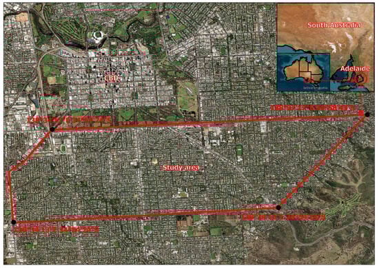
Figure 1.
location of the study area in Adelaide, city, Australia.
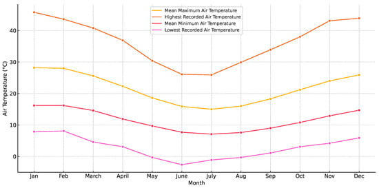
Figure 2.
Adelaide average annual thermal statistics between 1955 and 2024 (based on []).
While Adelaide’s climate is classified as temperate with hot, dry summers (Csa) under the Köppen–Geiger system [], this broad classification does not fully capture the city’s complex intra-urban thermal behaviour. Due to its geographic position in the lower mid-latitudes, Adelaide experiences extreme heatwaves driven by synoptic patterns originating in the mid-latitudes and influenced by tropical interactions [,,,]. These heatwaves are frequently associated with synoptic blocking systems, which prolong high-temperature episodes []. Previous studies have detected intra-urban heat island (IUHI) effects within Adelaide [,], although the city’s topography and the lack of a suitable rural station have made traditional UHI assessments difficult. Rogers et al. [] showed that Adelaide’s UHI intensifies under heatwave conditions—particularly during the night—indicating that urban morphology plays a critical role in local thermal amplification. Their findings suggest that during heatwaves, nocturnal UHIs are stronger than usual, while daytime UHIs may moderate slightly due to altered energy balance. These observations highlight the inadequacy of relying solely on general climate classifications and underscore the importance of mapping and analyzing the spatial distribution of heat within urban areas. The thermal heterogeneity observed across Adelaide reinforces the relevance of local-to-urban-scale studies that integrate land surface temperature, land use, and greening variables [].
Table 2.
Summary of land use–land cover in the study area.
Table 2.
Summary of land use–land cover in the study area.
| Land Use–Land Cover Type | Area (km2) | Percentage (%) |
|---|---|---|
| Constructed buildings | 7.39 | 35.74 |
| Canopy cover | 5.61 | 27.13 |
| Local roads (Type 1) | 3.89 | 18.81 |
| Regional roads (Type 2) | 0.27 | 1.31 |
| State roads (Type 3) | 0.44 | 2.13 |
| Residential (Type 1) | 17.34 | 83.85 |
| Commercial (Type 2) | 1.24 | 5.99 |
| Educational (Type 3) | 0.50 | 2.42 |
| Medical (Type 4) | 0.39 | 1.89 |
| Industrial (Type 5) | 0.01 | 0.05 |
| Parkland (Type 6) | 0.98 | 4.74 |
| Others | 0.14 | 0.68 |
2.2. Methodology
2.2.1. Data Acquisition
Various datasets were used to classify road typologies, land types, and to quantify LST, CCP, and NDVI.
In South Australian Government Data Directory (Data.SA), a Government web portal, the spatial layers relevant to CCP, LST, and NDVI were obtained []. The data produced in this portal include thermal imagery, tree canopy boundaries (height > 3 m), green space (growing vegetation < 2 m, emerging trees and trees between 2 and 3 m in height, shrubs, and other mid-story), vegetation greenness using NDVI, permeable and impermeable surfaces, building footprints, and green space extents. The height data was determined via Light Detection and Ranging (LiDAR) with an average point density of 8 points per m2, a remote sensing approach scanning the surface of the Earth. The Heat Map was generated from data collected at 3000 m altitude under a clear sky from a purpose-built aircraft fitted with an aerial thermal sensor. Thermal imagery has been captured with a spatial resolution of 2 m × 2 m []. Each pixel shows the average LST as measured. The spatial resolution for the Canopy Height Model (CHM) is 0.5 m × 0.5 m. In pursuing our objectives, we used the Heat Map captured during the day on 10th March 2018 between 11 a.m. and 3 p.m., and the layer of tree canopy > 3 m height. This is a two-dimensional spatial layer derived from CHM representing the tree canopy above 3 m from point cloud captured by LiDAR.
Australian Bureau of Statistics (ABS) [] includes mesh blocks (the smallest geographic areas containing between 30 to 60 dwellings) that were used to obtain land uses. These were categorized as residential, commercial, industrial, parkland, education, hospital/medical, transport, water, and other categories where they could not be easily placed in one of the above classifications []. The ABS digital boundaries are produced in two formats: OGC GeoPackage or ESRI shapefile, and in Geocentric Datum of Australia 2020 (GDA2020) and Geocentric Datum of Australia 1994 (GDA94). The shapefile of mesh blocks, which were created in the year 2021 and GDA2020 (MB_2021_AUST_GDA2020), was used for the land use–land cover (LULC) data required for this research [].
Open Street Maps (OSM) [] is a collaborative, open-source, up-to-date, and accurate dataset creating and providing free maps of the world including roads, rivers, railways, and points of interest. The road data (polylines) for Adelaide from OSM (AdelaideOSM_2023) was extracted comprising road types, length, name, and ID. This data was used to classify roads into simplified road typology for analysis to fulfill the aims of this research.
2.2.2. Data Preparation
The input data inclusive of Mesh Blocks, OSM Adelaide Roads, and Tree Canopy are in vector format, while NDVI, Elevation, and Thermal Day Imagery are in rasters. These layers were used as essential inputs for processing through Geographic Information Systems (GIS) in the map projection of GDA2020_MGA_ZONE54 (Geocentric Datum of Australia 2020 for the research zone). Different sources and layers were used to prepare the data (Figure 3):
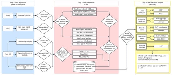
Figure 3.
Data flow diagram of steps applied in this study.
- 1.
- OSM Adelaide Roads were categorized into three classifications based on the three-tier hierarchy introduced in [] as Figure 4a shows. The term “typology” means the number of traffic lanes (width of roads). Type 1, 2, and 3 indicate local (2 lanes), regional (4 lanes), and state roads (6 lanes and over).
- 2.
- To analyze the impact of various factors on UHIULI mitigation, each road typology was segmented into uniform blocks at 100 m2 (in terms of area not dimensions (Figure 5)). This segmentation ensured that contributing factors could be quantified with minimal complexity and higher accuracy, leading to consistent results. The choice of 100 m2 blocks was driven by the need to isolate the cooling effects of identified factors while minimizing other influences such as orientation. To validate this approach, block sizes of 100, 500, and 1000 m2 were examined. However, for larger blocks, multiple land uses were often encompassed within a single unit, which complicated the assessment of land type effects. As a result, the 100 m2 block size was adopted as the optimal unit. In total, 4433 blocks were created and each block was assigned an ID, X and Y coordinates, elevation, and road typology.
- 3.
- From the data in the Mesh Block layer, 7 types of LULC were identified, including land type 1: residential, type 2: commercial, type 3: education, type 4: medical, type 5: industrial, and type 6: parkland. Each block of road typology was allocated a specific land type (Figure 4b). Our comparison is based on land use types adjacent to roads not as the built-up areas. Building areas (rooftops) were removed from the road areas considered in this analysis (explanation for building surface temperature was added).
- 4.
- TreeCanopy_Above3m is a vector layer (Figure 4c) that was used for measuring CCP. With the area of each block being 100 m2, CCP was calculated for each block based on road typology and integrated with land type.
- 5.
- NDVI values (mean NDVI) were calculated from the relevant layer (spatial resolution of 3 m × 3 m) in the Adelaide Heat Map dataset for each block with the certain CCP and land type (see Figure 4d). NDVI is included alongside CCP to assess not only the extent and shading of tree canopy cover but also its density, which influence evapotranspiration. While CCP measures the quantity of canopy cover, NDVI reflects canopy quality, distinguishing healthy or stressed, dense or sparse ones. Since areas with similar CCP can have varying cooling effects depending on tree health and greenness, incorporating NDVI provides a more accurate understanding of how canopy cover impacts LST [,,].
- 6.
- Mean LST (Figure 4e) for each block was extracted from ThermalDay imagery (spatial resolution of 2 m × 2 m) in GIS. This resulted in the average surface temperature of each block. The data was compiled into a database for further analysis.
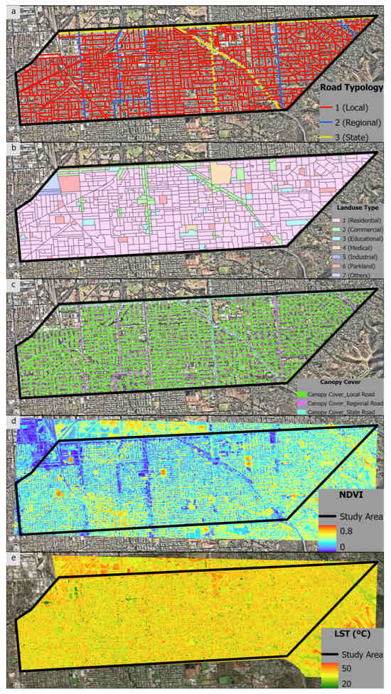
Figure 4.
Details of the research zone in Adelaide, Australia; (a) road typology, (b) land use type, (c) canopy cover, (d) NDVI, and (e) LST.
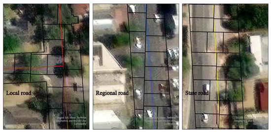
Figure 5.
Graphical illustration of a 100 m2 blocks for three road typologies.
2.2.3. Data Analysis
To determine the correlations between the contributing factors in this research, generalized additive models (GAMs) were utilized. With this statistical approach, we could analyze the key variables of LST with respect to various road typologies and adjacent land use types. GAMs extend generalized linear models (GLMs) by replacing linear relationships between predictors and the response variable with flexible, smooth functions of the covariates []. This flexibility enables GAMs to model nonlinear relationships between the predictors and the response variable while preserving the straightforward and understandable nature of additive models []. In GAMs, each predictor can be modeled using a smooth function, often represented using splines, like cubic splines, or other smoothing techniques. The overall model remains additive, meaning that the contribution of each predictor to the response variable is added together, which simplifies interpretation compared to more complex models like random forests or neural networks []. GAMs are particularly useful when nonlinear patterns are expected in the data, but overfitting needs to be controlled by carefully managing the smoothness of the functions [].
As different factors contribute to UHIULI, the GAM model was applied in this study to predict the LST based on several predictor variables (so-called independent variables in some regression models). In the prediction model, both linear predictors (CCP and NDVI) and categorical predictors (road typology and land types) were analyzed under two conditions. The first was without interaction, where each predictor was examined independently to assess its individual effect on LST. This included evaluating how CCP, NDVI, road typology, and land type contribute separately to variations in LST. The second was with interaction, where combined effects of the predictor pairs were explored to understand potential interactions. This involved analyzing the joint influence of CCP and NDVI, and joint influence of road typology and land use type to determine whether their co-effect amplifies or mitigates LST differently or not. However, to determine if there was an association between road typology and land type, which are categorical factors, Pearson’s Chi-squared test was applied and proved that the p-value is less than 2.2 × 10⁻¹⁶. This indicates a highly significant association between road typology and land type, meaning certain land type categories are more likely to occur with specific road typology categories. To reveal any dependency between NDVI and CCP, which are linear predictors, linear regression was applied, and as Figure 6 shows, there is a positive correlation between the CCP and NDVI values, meaning as CCP increases, NDVI values tend to rise and areas with more tree cover have healthier or denser vegetation. These associations highlight the need to consider the dependency between these variables to ensure accurate and reliable model estimates.
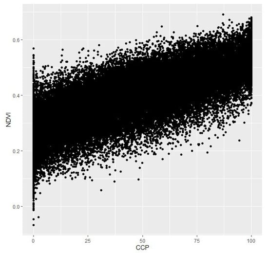
Figure 6.
The scatter plot of NDVI and CCP.
Given the explanation above, GAM was assigned to a model with spatial coordinates (X, Y) and elevation as smooth functions, CCP and NDVI as linear predictors, road typology (local, regional, and state) and land use types (residential, commercial, educational, medical, industrial, and parkland) as categorical predictor variables, and LST as a dependent or response variable. As we should examine the co-effects of linear and categorical predictors, the model also considered the interaction between these variables (Figure 3).
The model uses a t-distribution rather than a normal distribution to be more suitable for modeling the data as it has heavier trails compared to a normal distribution. The identity link function is also used to predict the response variable (LST) directly without transformation, and it is used to understand and the results.
Model:
GAM(LST ~ s(X,Y) + CCP*NDVI + factor(RoadType)*factor(LandType)
+ s(Elevation), family = scat(link = "identity"))
The deviance for the model explains 63.9% of deviance in the response variable (LST), which is quite high. In the model, ~means LST is a response variable depending on other factors; CCP(*NDVI) and factor (RoadType) * factor (LandType) indicate interactions between two linear predictors and categorical factors, respectively. The s(X,Y) and s(Elevation) indicate smooth functions of spatial coordination and elevation allowing the model to capture complex and nonlinear relationships with LST. The inclusion of s(X, Y) helps account for localized spatial variations in LST that may arise from the categorical and linear factors, while s(Elevation) captures potential nonlinear temperature changes associated with altitude. By using smooth functions, the model gains flexibility, improving its ability to accurately predict LST compared to a purely linear approach. For road typology and land type, as they are categorical variables, local road (road type 1) and residential land type (land type 1) were considered as the baselines whose effect is compared with that of the other types. The temperature difference for the statistical model throughout this paper is per 100 m2. The “family= scat” stands the scaled t-distribution which is useful for this paper’s model as the response variable (LST) has outliers. By applying this, t-distribution is less affected by extreme LST values and gives more stable estimates than a normal model. The “link= identity” is a standard identity link function, assuming a direct, untransformed relationship between the continuous response variable (LST) and the linear predictor and keeping. So, using family = scat (link = “identity”) helps the model provide robustness while ensuring straightforward interpretability.
Figure 7 and Table 3 present the distribution of the three continuous primary variables used in this study—LST, CCP, and NDVI—and provide a comprehensive overview of the landscape structure and thermal environment of the study area. The LST has a nearly normal distribution centred around a mean of 37.29 °C (SD = 3.21 °C), with values ranging from 21.76 °C to 49.09 °C. The median (37.36 °C), first quartile (Q1 = 34.91 °C), and third quartile (Q3 = 39.74 °C) are close to the mean, confirming the symmetric nature of the distribution. This suggests relatively consistent surface temperatures across the study area, potentially influenced by the uniformity of land use or surface materials. The CCP distribution is markedly right-skewed, with a significant proportion of observations clustered at or near 0%. This is reflected in the descriptive statistics, where the mean canopy cover is 41.18%, the median is slightly lower at 39.98%, and the first quartile is only 12.85%. Despite the maximum reaching 100%, the high standard deviation (30.54) and wide interquartile range indicate substantial spatial variability in canopy cover. The NDVI variable exhibits a moderately symmetric distribution with a peak around 0.38, closely aligned with its mean (0.37) and median (0.38). The NDVI values span from −0.07 to 0.69, with the interquartile range (Q1 = 0.29, Q3 = 0.46) capturing moderately vegetated areas. The relatively small standard deviation (0.12) suggests lower variability compared to CCP, indicating that while vegetation density varies, it is more consistent than canopy extent.
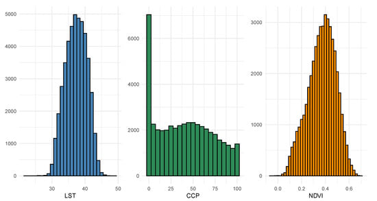
Figure 7.
Histograms of LST, CCP, and NDVI (Q8).
Table 3.
Main statistics of the variables.
3. Results
In the study area within the Adelaide region, the findings indicate that average LSTs are influenced by three types of variables—linear (CCP and NDVI), categorical (road typology, and land type), and smooth terms (spatial coordinates and elevation)—though the level of significance varies among them. Overall, the interaction (co-effect) between linear variables and between categorical variables contributes to changes in LST, and consequently (UHIULI), highlighting the importance of the individual effects of the predictors and their co-effects. Table 4 provides a summary of the variables analyzed, including their descriptions and statistical significance. The baseline is road type 1 (local roads), land type 1 (residential land use), CCP = 0 (no tree canopy), NDVI = 0, and LST = 42.78 °C. The baseline serves as a reference point for interpreting the effects of the variables in the model. In other words, all other predictors or effects in the model are deviations from this baseline. As an example, the cooling effect of road type 2 (regional road) and land type 2 (commercial) combination is 0.15 °C less than the baseline per 100 m2. In Table 4, the estimate represents the effect size of each predictor variable on LST, indicating both the direction (negative or positive) and magnitude of the relationship. The p-value assesses the statistical significance of the predictor’s contribution to LST changes, and is categorized into three levels: highly significant (p < 0.001), moderately significant (p< 0.01), and weakly significant (p< 0.05). Small p-values suggest strong evidence of influence on LST. The standard error (Std. Error) quantifies the uncertainty in the estimate, where smaller values indicate greater reliability and precision, while larger values suggest higher uncertainty.
Table 4.
Summary of predictor variables and their parametric details.
To assess the individual contribution of each predictor variable to LST, a set of partial models was also developed, each containing only one main predictor or interaction term. We then evaluated their performance using two statistical indicators: Adjusted R2 and Deviance Explained (%). These metrics reflect the extent to which each variable, in isolation, accounts for the variability in LST, with Deviance Explained also indicating the contribution level of each predictor variable. Table 5 summarizes the outcomes of these assessments. The level of contribution is visually highlighted using color shading: darker green tones represent stronger contributions, while darker red tones indicate weaker contributions. Among all predictors, the interaction term CCP * NDVI showed the strongest explanatory contribution, with an Adjusted R2 of 0.68 and 68.3% deviance explained. This highlights the substantial role of both the quantity and quality of vegetation in regulating LST. Other strong contributors include CCP alone (Adjusted R2 = 0.65 and 65.3% deviance explained) and NDVI (Adjusted R2 = 0.54 and 54.1% deviance explained). These results confirm that vegetation cover, especially when both CCP and NDVI are considered, is a critical factor in mitigating urban heat. In contrast, spatial coordinates s(X, Y), land type, and road type, as well as their interaction, exhibited notably weaker contributions, with deviance explained values below 10%. Elevation had a negligible effect (Adjusted R2 = 0.007; 0.79% deviance explained), suggesting its influence on LST is minimal in this urban context.
Table 5.
Summary of contribution levels of predictor variables.
3.1. Effect of Spatial Variation and Elevation on LST
The analysis shows that the location coordinate is significant to LST (Figure 8). The isolines in Figure 8 represent three-dimensional data in two dimensions and provide evidence for spatial variation of LST across the x and y axes. The pattern suggests that the study area has fluctuating LST values in relation to the solid black line, which represents the reference value of 27.6 °C. The dashed green lines indicate higher LST values, while the dashed red lines indicate lower LST compared to the reference line. These dashed lines correspond to one standard error above (green) and below (red) the reference value, illustrating where the LST is higher or lower, respectively. The clustering of lines suggests rapid changes or steep gradients in LST, while more widely spaced lines indicate more gradual changes in LST. The enclosed loops in certain regions represent the local maximum or minimum in LST. These changes in LST might reflect the influence of localized factors, such as the presence of vegetation (for example, parks or gardens).
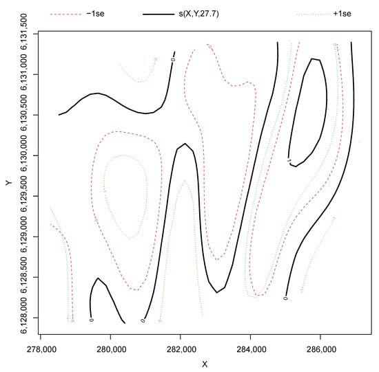
Figure 8.
Spatial variability by coordinates on LST.
The small p-value for elevation suggests that elevation is an important factor in predicting LST; however, the relationship is not linear and may be more complex, with LST potentially increasing or decreasing at different rates in different elevations. Higher elevations are generally expected to be cooler due to decreased atmospheric pressure, and vice versa []. Elevation in the area ranges from 23 to 178 m and the graph shows an almost uniform spread of LST along this area, with clustering of LST between 30 and 45 °C. This suggests that there is a moderate correlation between elevation and LST, as mentioned in other studies [,,].
3.2. Effect of Road Typology and Land Use and Land Cover on LST
Figure 9 shows the median LST across the three road typologies. The data suggests that a difference in surface temperature exists relative to the road type. Local roads (type 1) reported a median LST of 36.98 (range of 25.21 to 49.09 °C with a mean LST of 36.95 °C), showing the lowest variability compared to the other road types. Regional roads (type 2) reported a slightly higher median LST of 39.51 °C (range of 28.41 to 45.6 °C, mean LST = 38.70 °C). For state roads, the median LST was 39.98 °C (range of 21.76 to 46.79 °C, mean 39.35 °C). Regional and state roads reported higher LST values, with a greater concentration on LST in the middle to upper range compared to local roads. The statistical model and Table 4 suggest that regional and state roads generally have lower temperatures of 0.62 and 0.77 °C (Estimate column in Table 4) than local roads. The effect of road typology (width of roads) on LST is statistically significant (small p-value in Table 4) with precise estimates (small Std.error in Table 4).
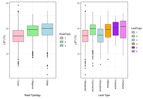
Figure 9.
Distribution of LST over road typology (left) and land type (right).
Figure 9 represents LST variation across land types. For residential land use (Type 1), the median LST is 37.04 °C, and it has a wide range from 21.76 to 49.09 °C. Commercial land use (Type 2) has a higher median of 39.91 °C, with a minimum of 25.21 and maximum of 46.54 °C. Educational land use (Type 3) has a minimum, median, and maximum LST of 25.76, 37.32, and 44.79 °C. The median for medical land use (Type 4) is 39.5 °C, showing slightly higher temperatures compared to educational land use and also with a higher range from 27.78 to 46.84 °C. Industrial land use (Type 5) and parkland (Type 6) show the highest LST with a median of 40.18 and 40.73 °C and also maximum of 40.18 and 40.73 °C, respectively. The LST variation for parkland, however, is larger, starting from 29.9 °C compared to that of industrial land use with 33.19 °C. Parkland includes a greater proportion of lower LST. The statistical model and Table 4 also show that for commercial land use, LST is about 0.37 °C lower than areas classified as residential and this effect is statistically significant and reliable, assuming all other variables remain constant. Educational land use is associated with a 0.13 °C lower LST compared to residential. This effect is not as large as commercial land use, showing only marginal significance and less reliability. Medical land use is, similarly, associated with a 0.15 °C decrease in LST compared to residential land use, and the results showed a moderate significance. For industrial land use, the coefficient is 0.06 °C, meaning that LST is slightly higher than residential land use. However, this difference is neither statistically significant nor highly reliable, suggesting that any observed increase in LST could be due to random variation rather than a consistent pattern. In contrast, parkland is associated with a 0.11 °C increase in LST compared to residential land use. Although this result is marginally significant, its high precision indicates that the observed difference is likely consistent and may reflect a real-world phenomenon. This could mean that parkland, despite being a green space, might absorb or retain heat more than what is expected due to factors like vegetation species, soil composition, the presence or patterns of irrigation, or lack of canopy shading impacting on the health of the underlying ground cover.
Figure 10 illustrates the effect of interaction between road typology and land type on mean, minimum, and maximum LST in the research area. Local–residential type (1-1) has the highest maximum LST (49.1 °C) but the second lowest mean LST (36.8 °C). However, the lowest minimum LST of residential belongs to the state–residential type (3-1) with 21.8 °C. Although local–parkland type (1-6) has the lowest mean LST (36.4 °C), this value is the highest for state–parkland (3-6) (41.2 °C). State–education type (3-3) has both the lowest mean and maximum LST with 36.4 and 41.7 °C, respectively. Local–industry type (1-5) has the highest minimum LST of 33.2 °C and a high mean and maximum LST value (39.8 and 45 °C). Interestingly, the maximum value for this combination is similar to that of local–parkland (1-6) and is even lower than that of state and regional–parkland types (3-6 and 2-6). The combination of parkland (6) with three road typologies does not have the lowest minimum LST (22.9 °C) when compared to the range of minimum LST values from 22.5 to 32.5 °C.
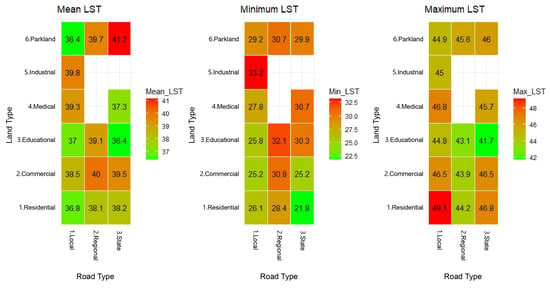
Figure 10.
The co-effect of road typology and land type on LST (note: 1. white spaces mean no data; 2. unit for LST is °C; 3. scale is different for each heat map).
As discussed in Section 2.2.3 and presented in Table 4, local road and residential land type are considered as a baseline (estimate = 0) to enable a comparison of other combinations impacting LST. The co-effects (Table 4) on LST are listed as follows:
Regional roads with adjoining commercial land use have a coefficient of 0.15, while the individual coefficients of regional road and commercial land type are −0.62 and −0.37, respectively. That means for this combination, LST is calculated by summing their individual and the interaction coefficients. In doing so, the effect will be adding these values together (−0.62 −0.37 +0.15), resulting in a total effect of −0.84. This indicates that on average, the combination of a regional road with commercial land use reduces LST by 0.84 °C when compared to local road with residential land use. The effect of this combination is marginally significant (typically not highly significant (at the 5% level) but marginally significant (at the 10% level)) and the estimate is relatively precise. This suggests a weak effect that lacks precision, meaning that the effect in reality might be different.
Regional roads with educational land use have a coefficient of 0.8, showing a 0.05 °C increase in LST (−0.62 −0.13 +0.8) for the interaction compared to that for local roads and residential land use. This result is highly significant but has relatively weak precision. This indicates variability in this effect, meaning that while road type 2 in land type 3 generally tends to increase LST, the actual increase may fluctuate around this estimate.
Regional roads with parkland land use show a coefficient of 0.34 that indicates a 0.17 °C decrease (−0.62 +0.11 +0.34) in LST due to the interaction compared to the baseline with moderate significance and reliability. However, the relatively high standard error implies some variability in this effect, meaning that the precise decrease in LST could range slightly.
State roads with a commercial land use are associated with a coefficient of 0.6, causing a 0.54 °C decrease in LST (−0.77 −0.37 +0.6) compared to local roads with residential land use. This combination has very strong significance and relatively strong estimated precision. This low error suggests a higher confidence in the impact on LST, meaning road type 3 (state) in land type 2 (commercial) is consistently associated with lower temperatures.
State roads with an educational land use reported a coefficient of −1.03 and are associated with a 1.93 °C decrease in LST (−0.77 −0.13 −1.03) compared to the combination of local roads and residential land use with strong significance and weak precision. The relatively large error means that while road type 3 (state) with land type 3 (educational) is associated with cooling, the precise amount of cooling varies more in this combination than in others.
State roads with medical land use reports a coefficient of 0.51, indicating a 0.41 °C decrease (−0.77 −0.15 +0.51) in LST for this interaction compared to that for local roads and residential land use, and the result is highly significant but not with a high precision. The observed value for the interaction term might be due to increased heat retention in areas with road type 3 (state) and land type 4 (medical). However, the effect size varies moderately, meaning the temperature reduction is significant but not consistent across all locations.
State roads with parkland land use report a coefficient of 1.28, showing a 0.62 °C increase in LST (−0.77 +0.11 +1.28) compared to the interaction between local roads and residential land use. This is highly significant with moderate reliability. This strong and relatively stable effect is likely due to the characteristics of road type 3 (state) and land type 6 (parkland) areas that are more exposed to sun and retain more heat.
3.3. Effect of CCP and NDVI on LST
Figure 11 illustrates that both CCP and NDVI appear to be negatively correlated with LST. This suggests that areas with higher values of CCP and NDVI are associated with lower LST, and increasing CCP and NDVI along all road typologies is an effective strategy for reducing UHIULI. However, the relationship between NDVI and LST appears to exhibit a stronger rate of change (steeper gradient) compared to the relationship between CCP and LST. This could indicate that NDVI, at lower values, is more sensitive to changes in LST. NDVI measures the difference between near-infrared light, which vegetation strongly reflects, and red light, which vegetation absorbs for photosynthesis. Lower NDVI values (typically up to 0.5) suggest stressed, sparse, or unhealthy vegetation []. NDVI is a well-known indicator of vegetation health and greenness [,]. This result suggests that if linear green infrastructure is to be applied as a UHI cooling strategy, the greatest gains will be made if this vegetation is supported by irrigation to improve its health, particularly where hot and dry summer climates prevail. The results also suggest that CCP and NDVI may have a more significant role in attenuating UHI along linear green infrastructure. Table 4 reports, for every 1% increase in CCP, LST decreases by about 0.05 °C, holding other variables constant. For every unit increase of 0.1 in NDVI, LST decreases by about 0.72 °C. Regarding Table 4, the estimated coefficient for CCP is more reliable than that of NDVI, as indicated by its smaller standard error. However, both variables exhibit a highly significant cooling effect on LST (p < 0.001). Additionally, CCP and NDVI are strongly interrelated, meaning that an increase in canopy cover generally leads to a higher NDVI and vice versa.
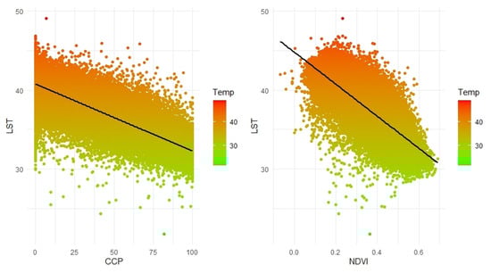
Figure 11.
The relationship of CCP and NDVI with LST (note: unit for LST is °C).
Figure 12 illustrates the 3D scatter plot of co-effect of CCP and NDVI on LST within road typology. The cluster of points suggests that higher LST values (red points) tend to occur when CCP is lower and potentially when NDVI is also lower. This reflects the absence of vegetation, which often leads to higher temperatures. Conversely, lower LST values (green points) are associated with higher CCP and higher NDVI values, demonstrating that areas with more canopy cover and greener or denser vegetation tend to be cooler. The cooling effect from the trees may still help keep LST lower than areas with no canopy at all, but LST could be higher than in areas where both CCP and NDVI are low. The LST could be relatively low even with lower CCP. Table 4 reports the output from the statistical model where the interaction term between CCP and NDVI provides a negative coefficient of −0.03. This means that increasing both CCP and NDVI simultaneously by one unit declines LST by 7.75 °C (−0.5 −7.22 −0.03 = −7.75), which is more effective than CCP (−0.5) and NDVI (−7.22) separately, and the estimated coefficient is highly precise.
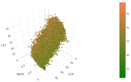
Figure 12.
Co-effect of CCP and NDVI on LST (note: unit for LST is °C).
By comparing Figure 10 and Figure 13, the joint effect of canopy coverage, vegetation density, and health on LST with road–land type interaction can be assessed. For example, the combination of a relatively high CCP (46.3%) and NDVI (0.40) in the context of a local road and residential land use yields one of the lowest mean LST values, at 36.8 °C. Similar patterns are observed for local roads with parkland and educational land use, as well as for state roads with medical land use. However, in contrast, the combination of a local road with residential land use also produces the highest recorded maximum LST, at 49.1 °C. The “hot spots” in these areas are attributed to lower canopy cover. In cases where both CCP (9.2%) and NDVI (0.22) are low, such as in state roads with parkland, the highest mean LST (41.2 °C) is observed. This indicates that grassy areas with limited canopy shading and a higher level of brown vegetation rather than green contribute significantly to the urban linear heat effect (UHIULI). Interestingly, combinations with relatively high CCP (45%) but lower NDVI (0.30)—such as state roads with educational land use—result in a lower mean LST (36.4 °C) compared to state roads with commercial land use, which have slightly lower CCP but higher NDVI (37.3 °C). Further comparison of the NDVI values in the state road and parkland combination and the regional road and commercial combination, both of which share a CCP of 9.2%, reveals that despite having a lower NDVI, the regional–commercial combination exhibits lower mean and maximum LST values than the state road–parkland combination.
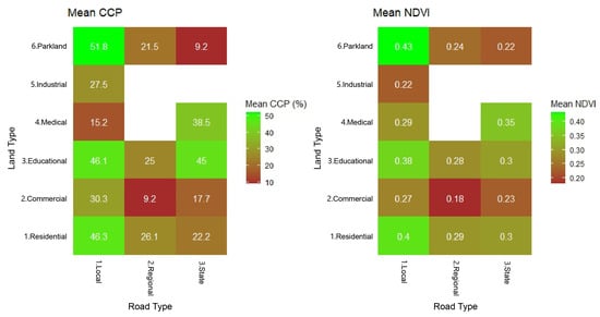
Figure 13.
Distribution of CCP and NDVI over road typology and land use type (note: 1. white spaces mean no data; 2. scale is different for each heatmap).
4. Discussion
4.1. Road and Land Type
The results of this study report that as roads become wider, there is a greater sky view factor (SVF) and a lower aspect ratio (AR); LST declines and becomes cooler when other factors are constant. Regional roads (type 2) have an average LST 0.62 °C lower and state roads (type 3) 0.76 °C lower than local roads (type 1) per 100 m2. This result is inconsistent with the study by Junsik Kim et al. [] who reported that an increase of 0.08 in SVF causes the urban canyon surface to receive a greater level of radiation resulting in 0.64 °C higher average LST. However, other studies [,] report that as urban canyons become narrower, multi vortices appear, causing more complicated airflow and weaker ventilation and heat removal at near-ground level and leading to higher LST. In this research, decreased LST may be due to the proximity of road typologies to different land use types or predominant orientation. Some sections of state roads in the northern part of the study area are adjacent to parkland or regional roads and primarily follow north–south orientation, while local roads exhibit more varied alignments.
In terms of lowest to highest LST values, land types can be ordered as commercial (−0.37 °C), medical (−0.15 °C), educational (−0.13 °C), residential (0), industrial (0.05 °C), and parkland (0.11 °C). Other studies [] have reported that the residential land use type has a lower LST than commercial, medical, and educational land uses. Marco Morabito et al. [] also reported 0.5 °C cooler LST in residential areas than parkland areas. These studies reported that the variation in LST adjacent to the residential land use type could be explained by the different percentage of pervious surfaces and green fragmentation integrated with this land use. This study, however, did not analyze the percentage of pervious or impervious surfaces, so we are uncertain whether this explanation holds for Adelaide.
Commercial land use is estimated to have the lowest LST in this area, at 0.37 °C lower than residential land use (Table 4). This result differs from other studies [,] that report elevated LSTs across commercial areas relative to residential land. However, lower LSTs have been reported in dense commercial land use in the USA and China [,,]. They highlighted that high-rise commercial buildings and complexes can provide greater amenities like green spaces, walking and cycling tracks, and also good public transport access around them. This open space may decrease anthropogenic heat emissions which was not considered in our study. However, in this study area, commercial land use types are mostly adjacent to state and regional roads (which are cooler than local roads), particularly those sections near parkland areas.
Educational land use type experiences a cooler LST by 0.13 °C per 100 m2 compared to residential land use (Table 4). Our results differ to those obtained by Haizhen Wen et al. [], who note that educational land use contains various facilities such as air conditioning or mechanical ventilation systems producing heat emissions even in suburbs causing increased LST compared to the others. However, Xincheng He [] reported that densely vegetated areas around schools in this land type could reduce average local LST by a maximum of 0.5 °C in varying districts of China. The researchers also pointed out that local climate zones and local urban morphology could apparently contribute to LST values in educational lands. For example, compact mid-rise, large low-rise, bare paved or soil areas, higher building and road density, greater floor area ratio, and artificial surfaces elevate LST, while dense or scattered-tree areas, and high SVF mitigate LST. These findings align with our study, as educational land uses in the study area are located in open spaces, primarily grassed, and surrounded by canopy cover.
Medical land type, consisting of hospitals of different sizes, reports a cooler LST by 0.15 °C compared to the residential land type. Chen et al. looked at this land use but amalgamated with schools, cultural, political, and sport facilities []. Their study revealed that mean LST over this land type was 0.64 °C less than the commercial type and 0.25 °C higher than the residential type because of different levels of surrounding green infrastructure. Figure 10 and Figure 13 indicate that while the educational land type does not show the highest vegetation values, it remains one of the most well-vegetated areas across all road typologies in this study area. This likely explains its lower LST compared to residential land uses.
Industrial land types report an LST 0.05 °C higher than residential areas. This is the smallest temperature difference (compared to the baseline) when comparing land use types. In [,], the highest LST is reported in industrial zones, including suburban regions characterized by extensive, contiguous industrial areas. However, in [], industrial zones with substantial vegetated areas exhibit a lower recorded LST. This is consistent with Figure 10 and Figure 13, which show that although industrial land uses have a slightly lower mean NDVI than medical land uses by 0.07, its 12.3% higher CCP results in similar LST values. In this study, industrial land use occupies the significantly smallest area and has the least proximity to the road typologies compared to the others (Table 2). This limited spatial extent may contribute to its lower average LST compared to other land uses and parkland in particular.
Table 4 also shows that parkland is estimated to be the hottest land type over road typologies, showing 0.11 °C higher than residential LST. This contrasts with other studies [,,,] reporting parkland as offering a cooling island in urban areas with 1–10 °C lower LST. The results in [] imply a cooler mean LST of parkland by 2.48, 2.1, and 3.26 °C compared to residential, public services (schools, hospitals, sport facilities), and commercial land use, respectively. However, these differences declined to 0.6, 0.85, and 1.98 °C for brownfield, which was defined as unused lands or wastelands. According to these studies [,,,], the cooling effect of parkland strongly depends on factors like their distance to the city center, CCP, NDVI, and intended use such as public gardens, local parks, or sport fields. In our study, the lands categorized as parkland that were adjacent to regional and state roads had little grass, often bare soil, and contained little or no canopy cover (mean CCP of 9 and median CCP of 0 for state roads, mean CCP of 21 and median CCP of 2.6 for regional roads). Further, it was likely that these parks had no or poor irrigation, which resulted in a low NDVI value (mean and median of 0.2 compared to NDVI for healthy and green vegetation being 0.66 and more []). These values indicate the importance of maintaining healthy vegetation and canopy trees to provide shading if parks are to be used as a mitigation strategy to lessen the UHI effect.
4.2. CCP and NDVI
GAM analysis shows if CCP increases by 1% on a road, LST can decrease by 0.05 °C. For example, by increasing 60% of CCP, a 3 °C reduction in LST would occur. This correlation is in line with another study on a Mediterranean climate conducted in Portugal where areas with CCP larger than 70% experience 3.42 °C cooler LST than those between 10 and 30% []. Other studies [,] also show that CCP is a reliable contributing factor to LST mitigation because it can significantly mitigate solar short-wave radiation penetrating deeply under canopy. Combined with the evapotranspiration of canopy trees, this leads to higher latent heat flux compared to the sensible heat experienced in non-canopy areas, ultimately lowering LST.
As reported in Table 4, every increase of 0.1 in NDVI value can cause a 0.72 °C decline in LST, which is one of the most significant predictors, as suggested by the p-value. This is consistent with other research [] that reports that higher greenness leads to lower LST. Some studies indicate a stronger correlation between NDVI and LST, such as a 19% decrease in NDVI that can increase LST by 7.2 °C [] or an increase in NDVI by 0.87 that leads to a decrease of 13.44 °C in LST []. This negative correlation between NDVI and LST tends to be stronger in summer, indicating that higher NDVI suggests well-irrigated green canopy cover and lower LST [].
Values resulting from the interaction between CCP and NDVI indicate that this combination has a more significant cooling effect on LST with strong confidence across our data, meaning this reliably leads to a reduction in LST. This cooling effect may be influenced by other factors like urban morphology but always remains in a negative correlation with UHIULI, in contrast to road–land interaction, which changes from separated to combined analysis and from one combination to another even in the same area. Unfortunately to date, existing studies’ focus has been on the effect of either canopy cover structure or NDVI separately on UHI because the multi-variate regression model considers multiple inputs, leading to duplicated contributions from these layers, and there is a paucity of knowledge that considers this co-effect on LST in urban systems and urban linear systems. Although CCP and NDVI are dependent, the canopy cover percentage (CCP) represents the proportion of tree crown coverage within each road block, thus capturing the vertical shading and physical coverage directly above road surfaces. In contrast, NDVI reflects overall vegetation greenness and photosynthetic activity, including ground-level vegetation (shrubs, grasses, lawns) in addition to trees, which are strongly related to evapotranspiration processes contributing to surface cooling. Including both variables allows the model to consider both the structural shading effects (CCP) and the vegetation density effects (NDVI), which together provide a more comprehensive representation of vegetation’s influence on land surface temperature. Thus, including both CCP and NDVI allows us to capture complementary mechanisms of urban heat mitigation: structural shading and evapotranspirative cooling (explanation for CCP and NDVI dependency was added).
As this research reveals, the role of road–land type in UHIULI mitigation is complex because of a wide range of geographical and environmental factors. This complexity suggests that the application of green infrastructure or nature-integrated-based solutions to achieve urban cooling may not necessarily achieve the desired temperature reduction outcomes []. For example, according to Zheng et al. [], LST in local–residential use type is impacted by both the height of buildings and vegetation coverage along roadways, while Chen et al. [] revealed that in parkland, industrial, and commercial land use in Berlin, Germany, LST is more affected by built environment factors like shading, materials, or anthropogenic heat, and in other land uses, NDVI is a dominant contributing factor to varying LST. This study, however, did not consider road typology and other relevant characteristics such as SVF for the land type under research in Berlin.
Our research provides a statistical model tested for the analysis of the key factors influencing UHIULI mitigation, integrating built types (road characteristics and land use) and land cover types (canopy cover quantity and quality, elevation, and coordinates) to explore correlations between these factors and UHI magnitude, measured by LST. We found that the impact of road typology and land type on LST varies due to the complexity of urban systems and services. However, the cooling effect of canopy cover, as part of natural systems, is consistently significant, mitigating the thermal effects of built and human systems []. Furthermore, from a practical perspective, urban green strategies can be applied to roads more easily when compared to other approaches such as changing the surface albedo or the design of the road [,,]. From [], Adelaide tree canopy coverage increased by approximately 4% between 2019 and 2022, particularly along local streets. However, localized areas of vegetation loss persist, primarily where construction demand is high and along road typologies undergoing infrastructure upgrades. This duality underscores the complex challenges of balancing urban development with environmental sustainability and the urban energy budget, especially in the face of intensifying heat waves.
To optimize heat mitigation policies and improve financial management, it is essential to consider land use, land cover, and road typology. This research has the following limitations. The available data on linear infrastructure remains generic and could not fully capture the uniqueness of all urban sites, limiting the precision of road typology classification. Additionally, there remains a significant knowledge gap in heat mitigation strategies for linear infrastructure, complicating direct comparisons of our findings with previous studies. Nonetheless, this paper addresses the most critical factors and contributes to advancement of knowledge in urban heat mitigation.
Further, the study relied solely on the Adelaide database, which is a single-day thermal image (under consistent meteorological conditions, using a high-resolution thermal dataset collected on a cloud-free day under peak summer heat), and constrained the analysis to the availability of data, including LST, NDVI, and CCP (explanation about thermal image limitation was added). This limitation may have increased the uncertainty of the results, as some significant factors, such as canopy tree species, leaf area index (LAI), pavement materials, and local air temperature records, could not be considered. For instance, NDVI values can reflect prior weather conditions like rainy weather, potentially affecting their accuracy as indicators. In this dataset also, NDVI is calculated from vegetation with all heights but CCP reflects only above-3m canopy trees, resulting in some discrepancies such as high CCP and low NDVI. The research employed a remote sensing approach to examine UHIULI effects in Adelaide’s road networks during summer, relying on aerial imagery. One of the core contributions of this research is to propose a method for estimating the urban heat island effect specifically along road networks (UHIULI), which remains an unexplored component of the broader UHI phenomenon. The intention is not to generalize across all urban surfaces, but rather to offer a replicable framework for analyzing and mitigating heat exposure along linear infrastructure, where cooling interventions can have direct spatial and functional relevance. While this method was effective for large-scale analysis, more significant findings may emerge from similar studies conducted in experimental contexts. Future research could include logging local air temperatures along roads to enable surface–air temperature correlations and exploring new approaches or research directions that provide deeper insights into the effectiveness of urban heat mitigation strategies—particularly regarding tree canopy attributes such as crown width, height, species, and other types of vegetation cover. Additionally, with access to comparable databases, the methods and results of this study could be tested in cities with similar or contrasting climates, potentially enhancing their applicability and robustness.
5. Conclusions
In addressing three main questions, this research investigates how roads, crucial elements of urban linear infrastructure, can be converted into cool corridors. It examines the role of canopy cover percentage (CCP) in reducing land surface temperature (LST), explores the impact of additional contributing factors, and assesses the possibilities for optimizing CCP to enhance cooling effects. To explore these questions, remote sensing and statistical analysis approaches were applied. We first categorized roads into three types—local, regional, and state roads—and identified key factors such as canopy cover (percentage and NDVI) and land type (residential, commercial, educational, medical, industrial, and parkland). Then, we examined how LST varied under the combined influences of CCP, NDVI, and land type across different road typology and analyzed correlations between these variables and LST.
Unlike previous studies that examined canopy cover and NDVI separately, this research assesses their combined effect on LST. The findings highlight that interactions among contributing factors complicate the determination of optimal cooling values. While CCP and NDVI consistently show a negative correlation with LST, the combined effect of land type and road typology is more variable. These results underscore the complex interplay between built and natural environments, emphasizing the need for a multi-factor analysis rather than isolated assessments. While the absolute differences in LST between road types and land uses may appear numerically modest, even small reductions in surface temperature can have meaningful impacts on local heat dynamics. For example, a local road surface fully exposed to sunlight can reach 49 °C compared to a surface shaded 100% by tree canopy (28°C), representing a more than 10 degree difference, as shading reduces both incoming shortwave radiation and outgoing longwave re-radiation. Since roads constitute a large proportion of urban impervious surfaces, even marginal reductions in their surface temperature contribute cumulatively to lowering ambient air temperature, reducing heat stress, and improving human thermal comfort, particularly during heat waves (explanation for small difference was added).
Effective heat mitigation strategies require a holistic approach, where canopy cover along roads—the most influential factor—must be complemented by additional mitigation measures in adjacent land uses such as proper irrigation to support healthy green cover. Land use significantly affects LST, with commercial and medical areas exhibiting lower-than-expected temperatures due to green spaces and urban amenities. The interaction between road typology and land use further complicates temperature variations, as cooling effects depend on urban morphology and vegetation cover. While specific canopy cover percentages may provide significant cooling in some land uses, different configurations may be necessary in others. Therefore, the quantity of the canopy cover (CCP), its quality or health (NDVI), and strategic placement (relative to land type and road typology) of canopy trees are key determinants in mitigating UHI effect.
From a policy-making standpoint, urban linear heat is a built–natural environment phenomenon that is complex. Thus, coordination across various professional disciplines that have leverage on how roads, land use, and greening are planned and maintained is needed if urban cooling is to be achieved. We also note the need for additional research to further understand the effectiveness of urban heat mitigation strategies, particularly in relation to how the tree canopy (crown width, height, and species) and other vegetation cover can support UHIULI mitigation strategies.
Author Contributions
Conceptualization, E.M. and P.D.; methodology, E.M., P.D., M.C. and G.S.; software, E.M., M.C. and G.S.; validation, E.M. and M.C.; formal analysis, E.M., M.C. and G.S.; investigation, E.M., P.D., M.C. and G.S.; data curation, E.M. and M.C.; writing—original draft preparation, E.M.; writing—review and editing, P.D., M.C., G.S. and E.M.; visualization, E.M.; supervision, P.D., M.C. and G.S. All authors have read and agreed to the published version of the manuscript.
Funding
This research received no external funding.
Institutional Review Board Statement
Not applicable.
Informed Consent Statement
Not applicable.
Data Availability Statement
No new data were created in this study.
Conflicts of Interest
The authors declare no conflicts of interest.
Abbreviations
The following abbreviations are used in this manuscript:
| UHI | Urban Heat Island |
| ULI | Urban Linear Infrastructure |
| UHIULI | Urban heat within linear infrastructure |
| LST | Land Surface Temperature |
| CCP | Canopy Cover Percentage |
| NDVI | Normalized Difference Vegetation Index |
| Ta | Air Temperature |
References
- Phelan, P.E.; Kaloush, K.; Miner, M.; Golden, J.; Phelan, B.; Silva III, H.; Taylor, R.A. Urban heat island: Mechanisms, implications, and possible remedies. Annu. Rev. Environ. Resour. 2015, 40, 285–307. [Google Scholar] [CrossRef]
- Mirabi, E.; Davies, P.J. A systematic review investigating linear infrastructure effects on Urban Heat Island (UHIULI) and its interaction with UHI typologies. Urban Clim. 2022, 45, 101261. [Google Scholar] [CrossRef]
- Oke, T.R.; Mills, G.; Christen, A.; Voogt, J.A. Urban Climates; Cambridge University Press: Cambridge, UK, 2017. [Google Scholar] [CrossRef]
- Coutts, A.; Tapper, N. Trees for a Cool City: Guidelines for optimised tree placement. Melbourne Australia: Cooperative Research Centre for Water Sensitive Cities. CRC Water Sensitive Cities Sch. Earth Atmos. Environ. Monash Univ. 2017. Available online: https://watersensitivecities.org.au/wp-content/uploads/2017/11/Trees-for-a-cool-city_Guidelines-for-optimised-tree-placement.pdf (accessed on 1 July 2025).
- Santamouris, M.; Ding, L.; Fiorito, F.; Oldfield, P.; Osmond, P.; Paolini, R.; Prasad, D.; Synnefa, A. Passive and active cooling for the outdoor built environment–Analysis and assessment of the cooling potential of mitigation technologies using performance data from 220 large scale projects. Sol. Energy 2017, 154, 14–33. [Google Scholar] [CrossRef]
- Wong, N.H.; Jusuf, S.K.; La Win, A.A.; Thu, H.K.; Negara, T.S.; Xuchao, W. Environmental study of the impact of greenery in an institutional campus in the tropics. Build. Environ. 2007, 42, 2949–2970. [Google Scholar] [CrossRef]
- Droste, A.M.; Steeneveld, G.J.; Holtslag, A.A. Introducing the urban wind island effect. Environ. Res. Lett. 2018, 13, 094007. [Google Scholar] [CrossRef]
- Wei, G.; He, B.J.; Sun, P.; Liu, Y.; Li, R.; Ouyang, X.; Luo, K.; Li, S. Evolutionary trends of urban expansion and its sustainable development: Evidence from 80 representative cities in the belt and road initiative region. Cities 2023, 138, 104353. [Google Scholar] [CrossRef]
- Yu, Z.; Zhao, P. The factors in residents’ mobility in rural towns of China: Car ownership, road infrastructure and public transport services. J. Transp. Geogr. 2021, 91, 102950. [Google Scholar] [CrossRef]
- Oke, T.R. Canyon geometry and the nocturnal urban heat island: Comparison of scale model and field observations. J. Climatol. 1981, 1, 237–254. [Google Scholar] [CrossRef]
- Zhou, D.; Zhao, S.; Liu, S.; Zhang, L. Spatiotemporal trends of terrestrial vegetation activity along the urban development intensity gradient in China’s 32 major cities. Sci. Total Environ. 2014, 488, 136–145. [Google Scholar] [CrossRef]
- Irmak, M.A.; Yilmaz, S.; Dursun, D. Effect of different pavements on human thermal comfort conditions. Atmósfera 2017, 30, 355–366. [Google Scholar] [CrossRef]
- Gui, J.; Phelan, P.E.; Kaloush, K.E.; Golden, J.S. Impact of pavement thermophysical properties on surface temperatures. J. Mater. Civ. Eng. 2007, 19, 683–690. [Google Scholar] [CrossRef]
- Gedzelman, S.; Austin, S.; Cermak, R.; Stefano, N.; Partridge, S.; Quesenberry, S.; Robinson, D. Mesoscale aspects of the urban heat island around New York City. Theor. Appl. Climatol. 2003, 75, 29–42. [Google Scholar] [CrossRef]
- Kim, K.H.; Jeon, S.E.; Kim, J.K.; Yang, S. An experimental study on thermal conductivity of concrete. Cem. Concr. Res. 2003, 33, 363–371. [Google Scholar] [CrossRef]
- Gungor, S.; Cetin, M.; Adiguzel, F. Calculation of comfortable thermal conditions for Mersin urban city planning in Turkey. Air Qual. Atmos. Health 2021, 14, 515–522. [Google Scholar] [CrossRef]
- Oke, T.R. The energetic basis of the urban heat island. Q. J. R. Meteorol. Soc. 1982, 108, 1–24. [Google Scholar] [CrossRef]
- Cetin, M.; Adiguzel, F.; Zeren Cetin, I. Determination of the effect of urban forests and other green areas on surface temperature in Antalya. In Concepts and Applications of Remote Sensing in Forestry; Springer: Berlin/Heidelberg, Germany, 2023; pp. 319–336. [Google Scholar] [CrossRef]
- Rabl, A.; De Nazelle, A. Benefits of shift from car to active transport. Transp. Policy 2012, 19, 121–131. [Google Scholar] [CrossRef]
- Kilicoglu, C.; Cetin, M.; Aricak, B.; Sevik, H. Site selection by using the multi-criteria technique—A case study of Bafra, Turkey. Environ. Monit. Assess. 2020, 192, 1–12. [Google Scholar] [CrossRef]
- Cetin, M. The changing of important factors in the landscape planning occur due to global climate change in temperature, Rain and climate types: A case study of Mersin City. Turk. J. Agric.-Food Sci. Technol. 2020, 8, 2695–2701. [Google Scholar]
- Al-Wreikat, Y.; Serrano, C.; Sodré, J.R. Effects of ambient temperature and trip characteristics on the energy consumption of an electric vehicle. Energy 2022, 238, 122028. [Google Scholar] [CrossRef]
- Millard-Ball, A. The width and value of residential streets. J. Am. Plan. Assoc. 2022, 88, 30–43. [Google Scholar] [CrossRef]
- Doulos, L.; Santamouris, M.; Livada, I. Passive cooling of outdoor urban spaces. The role of materials. Sol. Energy 2004, 77, 231–249. [Google Scholar] [CrossRef]
- Feyisa, G.L.; Dons, K.; Meilby, H. Efficiency of parks in mitigating urban heat island effect: An example from Addis Ababa. Landsc. Urban Plan. 2014, 123, 87–95. [Google Scholar] [CrossRef]
- Zeren Cetin, I.; Ozel, H.B.; Varol, T. Integrating of settlement area in urban and forest area of Bartin with climatic condition decision for managements. Air Qual. Atmos. Health 2020, 13, 1013–1022. [Google Scholar] [CrossRef]
- Zeren Cetin, I.; Sevik, H. Investigation of the relationship between bioclimatic comfort and land use by using GIS and RS techniques in Trabzon. Environ. Monit. Assess. 2020, 192, 1–14. [Google Scholar] [CrossRef] [PubMed]
- Cetin, M. Climate comfort depending on different altitudes and land use in the urban areas in Kahramanmaras City. Air Qual. Atmos. Health 2020, 13, 991–999. [Google Scholar] [CrossRef]
- Cetin, M. Determination of bioclimatic comfort areas in landscape planning: A case study of Cide Coastline. AGRIS—Int. Syst. Agric. Sci. Technol. 2016, 4, 800–804. [Google Scholar]
- Fahmy, M.; Sharples, S.; Yahiya, M. LAI based trees selection for mid latitude urban developments: A microclimatic study in Cairo, Egypt. Build. Environ. 2010, 45, 345–357. [Google Scholar] [CrossRef]
- Gallay, I.; Olah, B.; Murtinová, V.; Gallayová, Z. Quantification of the cooling effect and cooling distance of urban green spaces based on their vegetation structure and size as a basis for management tools for mitigating urban climate. Sustainability 2023, 15, 3705. [Google Scholar] [CrossRef]
- Leuzinger, S.; Vogt, R.; Körner, C. Tree surface temperature in an urban environment. Agric. For. Meteorol. 2010, 150, 56–62. [Google Scholar] [CrossRef]
- Gachkar, D.; Taghvaei, S.H.; Norouzian-Maleki, S. Outdoor thermal comfort enhancement using various vegetation species and materials (case study: Delgosha Garden, Iran). Sustain. Cities Soc. 2021, 75, 103309. [Google Scholar] [CrossRef]
- Norton, B.A.; Coutts, A.M.; Livesley, S.J.; Harris, R.J.; Hunter, A.M.; Williams, N.S. Planning for cooler cities: A framework to prioritise green infrastructure to mitigate high temperatures in urban landscapes. Landsc. Urban Plan. 2015, 134, 127–138. [Google Scholar] [CrossRef]
- Abdollahzadeh, N.; Biloria, N. Outdoor thermal comfort: Analyzing the impact of urban configurations on the thermal performance of street canyons in the humid subtropical climate of Sydney. Front. Archit. Res. 2021, 10, 394–409. [Google Scholar] [CrossRef]
- Wang, L.; Su, J.; Gu, Z.; Tang, L. Numerical study on flow field and pollutant dispersion in an ideal street canyon within a real tree model at different wind velocities. Comput. Math. Appl. 2021, 81, 679–692. [Google Scholar] [CrossRef]
- Feldhake, C.; Danielson, R.; Butler, J. Turfgrass evapotranspiration. I. Factors influencing rate in urban environments 1. Agron. J. 1983, 75, 824–830. [Google Scholar] [CrossRef]
- Tan, C.L.; Wong, N.H.; Tan, P.Y.; Jusuf, S.K.; Chiam, Z.Q. Impact of plant evapotranspiration rate and shrub albedo on temperature reduction in the tropical outdoor environment. Build. Environ. 2015, 94, 206–217. [Google Scholar] [CrossRef]
- Dimoudi, A.; Nikolopoulou, M. Vegetation in the urban environment: Microclimatic analysis and benefits. Energy Build. 2003, 35, 69–76. [Google Scholar] [CrossRef]
- Monteith, J.; Unsworth, M. Principles of Environmental Physics: Plants, Animals, and the Atmosphere; Academic Press: Cambridge, MA, USA, 2013. [Google Scholar]
- Pauleit, S. Urban street tree plantings: Identifying the key requirements. In Proceedings of the Institution of Civil Engineers-Municipal Engineer; Thomas Telford Ltd.: London, UK, 2003; Volume 156, pp. 43–50. [Google Scholar] [CrossRef]
- Wong, N.H.; Yu, C. Study of green areas and urban heat island in a tropical city. Habitat Int. 2005, 29, 547–558. [Google Scholar] [CrossRef]
- Grace, J. 3. Plant response to wind. Agric. Ecosyst. Environ. 1988, 22, 71–88. [Google Scholar] [CrossRef]
- Mirabi, E.; Davies, P.J. Mitigating urban heat along roadways; systematic review of impact and practicability. Urban Clim. 2024, 58, 102207. [Google Scholar] [CrossRef]
- Sawka, M.; Millward, A.A.; Mckay, J.; Sarkovich, M. Growing summer energy conservation through residential tree planting. Landsc. Urban Plan. 2013, 113, 1–9. [Google Scholar] [CrossRef]
- Vailshery, L.S.; Jaganmohan, M.; Nagendra, H. Effect of street trees on microclimate and air pollution in a tropical city. Urban For. Urban Green. 2013, 12, 408–415. [Google Scholar] [CrossRef]
- Srivanit, M.; Hokao, K. Evaluating the cooling effects of greening for improving the outdoor thermal environment at an institutional campus in the summer. Build. Environ. 2013, 66, 158–172. [Google Scholar] [CrossRef]
- Souch, C.; Souch, C. The effect of trees on summertime below canopy urban climates: A case study Bloomington, Indiana. J. Arboric 1993, 19, 303–312. [Google Scholar] [CrossRef]
- Department, H.K.P. HKGBC Guidebook for Sustainable Built Environment. Hong Kong Planning Standards and Guidelines. Chapter 11: Urban Design Guidelines. 2015. Available online: https://hkgbc.org.hk/eng/resources/publications/HKGBC-Publication/Guidebook/HKGBC-Guidebook-for-Sustainable-Built-Environment.pdf (accessed on 22 August 2024).
- Ryliškė, J.; Puodžiukas, V.; Žilionienė, D. New Approach to the Lithuanian Road Classification Based on Worldwide Experience; VGTU Press: Vilnius, Lithuania, 2017; Available online: https://etalpykla.vilniustech.lt/handle/123456789/154999 (accessed on 22 August 2024).
- Stewart, I.D.; Oke, T.R. Local climate zones for urban temperature studies. Bull. Am. Meteorol. Soc. 2012, 93, 1879–1900. [Google Scholar] [CrossRef]
- Godinho, S.; Gil, A.; Guiomar, N.; Costa, M.J.; Neves, N. Assessing the role of Mediterranean evergreen oaks canopy cover in land surface albedo and temperature using a remote sensing-based approach. Appl. Geogr. 2016, 74, 84–94. [Google Scholar] [CrossRef]
- Gorgani, S.A.; Panahi, M.; Rezaie, F. The Relationship between NDVI and LST in the urban area of Mashhad, Iran. In Proceedings of the International Conference on Civil Engineering Architecture & Urban Sustainable Development, Tabriz, Iran, 27–28 November 2013; Volume 2013. [Google Scholar]
- Sun, D.; Kafatos, M. Note on the NDVI-LST relationship and the use of temperature-related drought indices over North America. Geophys. Res. Lett. 2007, 34, 1485. [Google Scholar] [CrossRef]
- Marzban, F.; Sodoudi, S.; Preusker, R. The influence of land-cover type on the relationship between NDVI–LST and LST-T air. Int. J. Remote Sens. 2018, 39, 1377–1398. [Google Scholar] [CrossRef]
- Khandelwal, S.; Goyal, R.; Kaul, N.; Mathew, A. Assessment of land surface temperature variation due to change in elevation of area surrounding Jaipur, India. Egypt. J. Remote Sens. Space Sci. 2018, 21, 87–94. [Google Scholar] [CrossRef]
- Green Adelaide. Urban Heat and Tree Canopy Mapping. 2024. Available online: https://www.greenadelaide.sa.gov.au/projects/urban-heat-and-tree-canopy-mapping (accessed on 22 August 2024).
- BOM. Adelaide: Geographic Information. 2017. Available online: http://www.bom.gov.au/water/nwa/2017/adelaide/regiondescription/geographicinformation.shtml#Gdescription (accessed on 22 August 2024).
- DEW. Urban Heat and Tree Mapping of Adelaide. 2024. Available online: http://spatialwebapps.environment.sa.gov.au/urbanheat/?viewer=urbanheat (accessed on 22 August 2024).
- Peel, M.C.; Finlayson, B.L.; McMahon, T.A. Updated world map of the Köppen-Geiger climate classification. Hydrol. Earth Syst. Sci. 2007, 11, 1633–1644. [Google Scholar] [CrossRef]
- BOM. Seasonal Climate Summary for Greater Adelaide, Product code IDCKGC23L0. In Greater Adelaide in Summer 2018–19: Warmer and Drier Than Average; Technical Report, Common Wealth; 2019. Available online: http://www.bom.gov.au/climate/current/season/sa/archive/201902.adelaide.shtml (accessed on 1 July 2025).
- BOM. Greater Adelaide in Summer 2022–23: Drier Than Average; Generally Warmer Days. 2023. Available online: http://www.bom.gov.au/climate/current/season/sa/archive/202302.adelaide.shtml (accessed on 26 August 2024).
- BOM. Monthly Climate Statistics. 2009. Available online: http://www.bom.gov.au/climate/averages/tables/cw_023090.shtml (accessed on 23 August 2024).
- Ossola, A.; Jenerette, G.D.; McGrath, A.; Chow, W.; Hughes, L.; Leishman, M.R. Small vegetated patches greatly reduce urban surface temperature during a summer heatwave in Adelaide, Australia. Landsc. Urban Plan. 2021, 209, 104046. [Google Scholar] [CrossRef]
- Cowan, T.; Purich, A.; Perkins, S.; Pezza, A.; Boschat, G.; Sadler, K. More frequent, longer, and hotter heat waves for Australia in the twenty-first century. J. Clim. 2014, 27, 5851–5871. [Google Scholar] [CrossRef]
- Pezza, A.B.; Van Rensch, P.; Cai, W. Severe heat waves in Southern Australia: Synoptic climatology and large scale connections. Clim. Dyn. 2012, 38, 209–224. [Google Scholar] [CrossRef]
- Tryhorn, L.; Risbey, J. On the distribution of heat waves over the Australian region. Aust. Meteorol. Mag. 2006, 55, 169–182. [Google Scholar]
- Parker, T.J.; Berry, G.J.; Reeder, M.J. The influence of tropical cyclones on heat waves in Southeastern Australia. Geophys. Res. Lett. 2013, 40, 6264–6270. [Google Scholar] [CrossRef]
- Guan, H.; Bennett, J.; Ewenz, C.; Benger, S.; Zhu, S.; Clay, R.; Soebarto, V. Characterisation, Interpretation and Implications of the Adelaide Urban Heat Island; Flinders University: Adelaide, Australia, 2013. [Google Scholar]
- Erell, E.; Williamson, T. Intra-urban differences in canopy layer air temperature at a mid-latitude city. Int. J. Climatol. A J. R. Meteorol. Soc. 2007, 27, 1243–1255. [Google Scholar] [CrossRef]
- Rogers, C.D.; Gallant, A.J.; Tapper, N.J. Is the urban heat island exacerbated during heatwaves in southern Australian cities? Theor. Appl. Climatol. 2019, 137, 441–457. [Google Scholar] [CrossRef]
- Carlos, B.K.; Veronica, S.; Scott, H.; Ehsan, S. The Potential for Urban Canopy Cover to Reduce Heat-Related Mortality in Adelaide. In Urban Overheating: Heat Mitigation and the Impact on Health; Springer: Berlin/Heidelberg, Germany, 2022; pp. 249–273. [Google Scholar] [CrossRef]
- Data.SA. Metropolitan Adelaide Tree Canopy and Built Environment 2018/2019 tp 2022. 2024. Available online: https://data.sa.gov.au/data/dataset/metropolitan-adelaide-tree-canopy-and-built-environment-change-detection-2018-2019-to-2022 (accessed on 22 August 2024).
- Seed Consulting Services Western Adelaide Urban Heat Mapping Project. Technical report, Seed Consulting Services, Airborne Research Seed Consulting Services, Adelaide, South Australia 2017. Available online: https://www.adaptwest.com.au/sites/adaptwest/media/pdf/western_adelaide_urban_heat_mapping_report-(2).pdf (accessed on 23 August 2024).
- ABS. Census Geography Glossary, Understanding Census Geography, Descriptions of All Geographies Available for 2021 Census Data. 2022. Available online: https://www.abs.gov.au/census/guide-census-data/geography/census-geography-glossary (accessed on 23 August 2024).
- ABS. Mesh Blocks, Australian Statistical Geography Standard (ASGS) Edition 3. 2021. Available online: https://www.abs.gov.au/statistics/standards/australian-statistical-geography-standard-asgs-edition-3/jul2021-jun2026/main-structure-and-greater-capital-city-statistical-areas/mesh-blocks (accessed on 23 August 2024).
- OSM. OpenStreetMaps. 2023. Available online: https://www.openstreetmap.org/edit#map=16/-33.77084/151.10624 (accessed on 23 August 2024).
- Fatemi, M.; Narangifard, M. Monitoring LULC changes and its impact on the LST and NDVI in District 1 of Shiraz City. Arab. J. Geosci. 2019, 12, 127. [Google Scholar] [CrossRef]
- Anbazhagan, S.; Paramasivam, C. Statistical correlation between land surface temperature (LST) and vegetation index (NDVI) using multi-temporal landsat TM data. Int. J. Adv. Earth Sci. Eng. 2016, 5, 333–346. [Google Scholar] [CrossRef]
- Hastie, T.J. Generalized additive models. In Statistical Models in S; Routledge: London, UK, 2017; pp. 249–307. Available online: https://www.taylorfrancis.com/chapters/edit/10.1201/9780203738535-7/generalized-additive-models-trevor-hastie (accessed on 22 August 2024).
- Wood, S.; Goude, Y.; Fasiolo, M. Interpretability in generalized additive models. In Interpretability for Industry 4.0: Statistical and Machine Learning Approaches; Springer: Berlin/Heidelberg, Germany, 2022; pp. 85–123. [Google Scholar] [CrossRef]
- Wood, S.N. Generalized Additive Models: An Introduction with R; Chapman and Hall/CRC: Boca Raton, FL, USA, 2017. [Google Scholar] [CrossRef]
- Wiley, M.; Wiley, J.F.; Wiley, M.; Wiley, J.F. GAMs. In Advanced R Statistical Programming and Data Models: Analysis, Machine Learning, and Visualization; Apress: New York, NY, USA, 2019; pp. 165–224. Available online: https://link.springer.com/book/10.1007/978-1-4842-2872-2 (accessed on 22 August 2024).
- Phan, T.N.; Kappas, M.; Tran, T.P. Land surface temperature variation due to changes in elevation in northwest Vietnam. Climate 2018, 6, 28. [Google Scholar] [CrossRef]
- Abubakar, B.A.; Abubakar, S.A. Effect of elevation on land surface temperature (LST) variation in Jos and Environs, Nigeria. Intercont. Geoinf. Days 2021, 2, 151–154. [Google Scholar]
- Vasyl Cherlinka. All You Need To Know About Index. 2024. Available online: https://www.eos.com/blog/ndvi-faq-all-you-need-to-know-about-ndvi/?utm_source=chatgpt.com (accessed on 22 August 2024).
- Vilcins, D.; Sly, P.D.; Scarth, P.; Mavoa, S. Green space in health research: An overview of common indicators of greenness. Rev. Environ. Health 2024, 39, 221–231. [Google Scholar] [CrossRef]
- Rhew, I.C.; Vander Stoep, A.; Kearney, A.; Smith, N.L.; Dunbar, M.D. Validation of the normalized difference vegetation index as a measure of neighborhood greenness. Ann. Epidemiol. 2011, 21, 946–952. [Google Scholar] [CrossRef]
- Kim, J.; Lee, D.K.; Brown, R.D.; Kim, S.; Kim, J.H.; Sung, S. The effect of extremely low sky view factor on land surface temperatures in urban residential areas. Sustain. Cities Soc. 2022, 80, 103799. [Google Scholar] [CrossRef]
- Yang, H.; Chen, G.; Wang, D.; Hang, J.; Li, Q.; Wang, Q. Influences of street aspect ratios and realistic solar heating on convective heat transfer and ventilation in full-scale 2D street canyons. Build. Environ. 2021, 204, 108125. [Google Scholar] [CrossRef]
- Chen, Q.; Cheng, Q.; Chen, Y.; Li, K.; Wang, D.; Cao, S. The influence of sky view factor on daytime and nighttime urban land surface temperature in different spatial-temporal scales: A case study of Beijing. Remote Sens. 2021, 13, 4117. [Google Scholar] [CrossRef]
- Morabito, M.; Crisci, A.; Georgiadis, T.; Orlandini, S.; Munafò, M.; Congedo, L.; Rota, P.; Zazzi, M. Urban imperviousness effects on summer surface temperatures nearby residential buildings in different urban zones of Parma. Remote Sens. 2017, 10, 26. [Google Scholar] [CrossRef]
- Lu, Y.; Yue, W.; Huang, Y. Effects of land use on land surface temperature: A case study of Wuhan, China. Int. J. Environ. Res. Public Health 2021, 18, 9987. [Google Scholar] [CrossRef] [PubMed]
- Chen, S.; Haase, D.; Qureshi, S.; Firozjaei, M.K. Integrated land use and urban function impacts on land surface temperature: Implications on urban heat mitigation in Berlin with eight-type spaces. Sustain. Cities Soc. 2022, 83, 103944. [Google Scholar] [CrossRef]
- Kim, J.I.; Jun, M.J.; Yeo, C.H.; Kwon, K.H.; Hyun, J.Y. The effects of land use zoning and densification on changes in land surface temperature in Seoul. Sustainability 2019, 11, 7056. [Google Scholar] [CrossRef]
- Stone, B.; Hess, J.J.; Frumkin, H. Urban form and extreme heat events: Are sprawling cities more vulnerable to climate change than compact cities? Environ. Health Perspect. 2010, 118, 1425–1428. [Google Scholar] [CrossRef]
- Chen, L.; Jiang, R.; Xiang, W.N. Surface heat island in Shanghai and its relationship with urban development from 1989 to 2013. Adv. Meteorol. 2016, 2016, 9782686. [Google Scholar] [CrossRef]
- Wen, H.; Xiao, Y.; Zhang, L. School district, education quality, and housing price: Evidence from a natural experiment in Hangzhou, China. Cities 2017, 66, 72–80. [Google Scholar] [CrossRef]
- He, X.; Gao, W.; Wang, R. Effect of urban structure on land surface temperature around elementary schools in Hangzhou based on local climate zones. Sustain. Cities Soc. 2024, 114, 105724. [Google Scholar] [CrossRef]
- Su, W.; Gu, C.; Yang, G. Assessing the impact of land use/land cover on urban heat island pattern in Nanjing City, China. J. Urban Plan. Dev. 2010, 136, 365–372. [Google Scholar] [CrossRef]
- Algretawee, H.; Rayburg, S.; Neave, M. Estimating the effect of park proximity to the central of Melbourne city on Urban Heat Island (UHI) relative to Land Surface Temperature (LST). Ecol. Eng. 2019, 138, 374–390. [Google Scholar] [CrossRef]
- Feng, Y.; Zhang, K.; Li, A.; Zhang, Y.; Wang, K.; Guo, N.; Wan, H.Y.; Tan, X.; Dong, N.; Xu, X.; et al. Spatial and Seasonal Variation and the Driving Mechanism of the Thermal Effects of Urban Park Green Spaces in Zhengzhou, China. Land 2024, 13, 1474. [Google Scholar] [CrossRef]
- Wang, X.; Cheng, H.; Xi, J.; Yang, G.; Zhao, Y. Relationship between park composition, vegetation characteristics and cool island effect. Sustainability 2018, 10, 587. [Google Scholar] [CrossRef]
- Jena, J.; Misra, S.R.; Tripathi, K.P. Normalized difference vegetation index (NDVI) and its role in agriculture. Agric. Food E-Newsl. 2019, 1, 387–389. [Google Scholar]
- Mildrexler, D.J.; Zhao, M.; Running, S.W. A global comparison between station air temperatures and MODIS land surface temperatures reveals the cooling role of forests. J. Geophys. Res. Biogeosciences 2011, 116, 1486. [Google Scholar] [CrossRef]
- Huband, N.; Monteith, J. Radiative surface temperature and energy balance of a wheat canopy: I. Comparison of radiative and aerodynamic canopy temperature. Bound.-Layer Meteorol. 1986, 36, 1–17. [Google Scholar] [CrossRef]
- Roberts, D.A.; Dennison, P.E.; Roth, K.L.; Dudley, K.; Hulley, G. Relationships between dominant plant species, fractional cover and land surface temperature in a Mediterranean ecosystem. Remote Sens. Environ. 2015, 167, 152–167. [Google Scholar] [CrossRef]
- Liu, L.; Zhang, Y. Urban heat island analysis using the Landsat TM data and ASTER data: A case study in Hong Kong. Remote Sens. 2011, 3, 1535–1552. [Google Scholar] [CrossRef]
- Zheng, Z.; Zhou, W.; Yan, J.; Qian, Y.; Wang, J.; Li, W. The higher, the cooler? Effects of building height on land surface temperatures in residential areas of Beijing. Phys. Chem. Earth Parts A/B/C 2019, 110, 149–156. [Google Scholar] [CrossRef]
Disclaimer/Publisher’s Note: The statements, opinions and data contained in all publications are solely those of the individual author(s) and contributor(s) and not of MDPI and/or the editor(s). MDPI and/or the editor(s) disclaim responsibility for any injury to people or property resulting from any ideas, methods, instructions or products referred to in the content. |
© 2025 by the authors. Licensee MDPI, Basel, Switzerland. This article is an open access article distributed under the terms and conditions of the Creative Commons Attribution (CC BY) license (https://creativecommons.org/licenses/by/4.0/).