Abstract
Generative adversarial networks (GANs) can rapidly predict urban environmental performance. However, most existing studies focus on a single target and lack cross-performance comparisons under unified conditions. Under unified urban-form inputs and training settings, this study employs the conditional adversarial model pix2pix to predict four targets—the Universal Thermal Climate Index (UTCI), annual global solar radiation (Rad), sunshine duration (SolarH), and near-surface wind speed (Wind)—and establishes a closed-loop evaluation framework spanning pixel, structural/region-level, cross-task synergy, complexity, and efficiency. The results show that (1) the overall ranking in accuracy and structural consistency is SolarH ≈ Rad > UTCI > Wind; (2) per-epoch times are similar, whereas convergence epochs differ markedly, indicating that total time is primarily governed by convergence difficulty; (3) structurally, Rad/SolarH perform better on hot-region overlap and edge alignment, whereas Wind exhibits larger errors at corners and canyons; (4) in terms of learnability, texture variation explains errors far better than edge count; and (5) cross-task synergy is higher in low-value regions than in high-value regions, with Wind clearly decoupled from the other targets. The distinctive contribution lies in a unified, reproducible evaluation framework, together with learnability mechanisms and applicability bounds, providing fast and reliable evidence for performance-oriented planning and design.
1. Introduction
How urban form determines environmental performance is a key question for rapid planning decisions [1]. In practice, assessments of wind, radiation, sunshine, and thermal comfort rely heavily on physical/numerical simulations [2], which are costly and time-consuming and therefore do not support fast, multi-objective iteration at the block scale [3]. By contrast, generative adversarial networks (GANs) can produce approximate results at a millisecond-to-second latency, offering a substantial advantage in timeliness [4,5,6]. Typical block-scale questions include whether opening a ventilation corridor will over-expose inner courtyards to summer radiation, how to secure winter sunshine on ground floors while avoiding excessive summer heat, and how to balance wind protection with air renewal in semi-enclosed plazas. Such decisions depend on the combined behaviour of outdoor thermal comfort (UTCI), annual solar irradiation (Rad), sunshine duration (SolarH), and near-ground wind speed (Wind). When assessed separately, these indicators can lead to contradictory design choices if their interactions are not explicitly understood, reinforcing the need for unified, multi-target evaluation.
Evaluating the predictive capability of GANs across different performance targets is therefore essential. However, the existing studies largely focus on single targets and pixel-level errors, lacking systematic cross-target comparisons and interpretable evaluations under unified conditions. Consequently, it remains unclear how reliability varies across targets, whether structural semantics are equally preserved, and how training efficiency and learning difficulty change with the target—questions that require answers under consistent data and evaluation protocols.
Under a combined-input and combined-protocol framework, this study systematically compares the predictive performance of pix2pix across four urban environmental targets—the Universal Thermal Climate Index (UTCI), annual solar irradiation (Rad), sunshine duration (SolarH), and near-ground wind speed (Wind). All four targets share the same urban-form raster, Xi’an Typical Meteorological Year (EPW) driver, homogeneous simulation toolchain, and multi-level evaluation metrics. In this way, the observed differences can be attributed to the physical nature and learnability of each target rather than to heterogeneous inputs or protocols. Side-by-side evaluations are conducted along four dimensions—pixel accuracy, structural/regional consistency, cross-task synergy, and training efficiency—and relative learnability is explained via the semantic complexity–error relationship. Experiments are performed on more than 2100 paired block-scale samples, with a reproducible reporting of time and epoch statistics. The paper is organised as follows: Section 2 reviews related work; Section 3 presents the methods, data, and the evaluation scheme; Section 4 reports the results and analysis; Section 5 offers a discussion and limitations; Section 6 concludes.
2. Literature Review
2.1. GAN-Based Prediction of Urban Environmental Performance
GANs provide an effective route to rapidly approximate the mapping of urban forms to environmental performance [7,8,9,10,11,12]. With urban form as the conditional input, the model directly generates performance maps for radiation, sunshine duration, thermal comfort, and wind fields, markedly reducing the inference latency and enabling design iteration and sensitivity analysis. Recent studies predominantly adopt pix2pix (U-Net + PatchGAN) or its multi-scale/attention variants for end-to-end translation and report second-level inference with pixel metrics outperforming traditional regressors on single-target tasks. Mokhtar et al. [13] used a conditional GAN to approximate OpenFOAM wind fields end-to-end, reducing the MAE to ~0.5–0.7 m/s on unseen geometries and enabling second-level feedback for early-stage wind comfort evaluations. Milla-Val et al. [14] used WRF fields as inputs and generated block-scale CFD-like wind fields with pix2pix, substantially accelerating year-round scenario assessments. Lu et al. [15] proposed SolarGAN to rapidly produce annual solar irradiation heatmaps from 2D urban data and verified the effects of terrain information and sample size on robustness. Zhang et al. [16] synthesised hourly façade irradiance time series using “occlusion fisheye images + a generative model,” matching physical truth in distribution and autocorrelation, with ~1–2 s per point generation.
However, most existing studies remain “single target, single metric, single scenario,” lacking systematic cross-target comparisons and interpretable evaluations under unified conditions. Inconsistencies in data sources, input encoding, and evaluation protocols hinder horizontal comparability; most works emphasise pixel metrics such as RMSE/SSIM, while overlooking structural/regional semantics and cross-target consistency; moreover, training efficiency and convergence trajectories are rarely reported in a standardised manner, obscuring engineering usefulness. Huang et al. [17] used pix2pix with a unified encoding to approximate pedestrian-level wind speed, annual irradiation, and UTCI, achieving second-level inference and ~100× acceleration and embedding GAN outputs into multi-objective optimisation, yet their data and evaluation were not a unified cross-target comparison, and structural/efficiency reporting remained insufficiently systematic. Consequently, a unified-input, unified-protocol comparison across UTCI, radiation/sunshine, and wind remains absent, and mechanistic explanations of relative learnability are even scarcer—precisely the gap addressed by this study.
2.2. Accuracy and Interpretability Evaluation of Deep Learning in AEC/Urban Applications
The evaluation of performance prediction is shifting from pure pixel errors to a joint emphasis on structural consistency and interpretability [18,19,20]. In architecture and urban planning contexts, RMSE/MAE/PSNR/SSIM alone cannot tell whether a model has truly learned boundaries, hot/cold regions, and spatial semantics; accordingly, more “structure-/perception-friendly” metrics and interpretability methods have been introduced in recent years: for example, Boundary IoU emphasises the sensitivity to boundary quality and cross-scale fairness, as shown by Cheng et al. [21], while LPIPS measures perceptual similarity via deep features that better align with human vision, as demonstrated by Zhang et al. [22]. Medical and remote-sensing evaluations also combine distance/boundary metrics with region-overlap metrics to achieve a more robust assessment of small targets and uncertain boundaries, as reported by Ostmeier et al. [23]. In terms of interpretability, reviews on city-scale energy and environmental modelling indicate that SHAP/LIME/PDP/ICE provide global and local causal cues, improving auditability and communicability in decision-making, as discussed by Darvishvand et al. [24]. However, the current evaluation landscape remains fragmented: metric definitions are non-uniform, cross-target synergy and consistency are weakly quantified, and analyses of learnability are largely missing. Even with Boundary IoU, LPIPS, or mixed boundary/region metrics, many studies still remain at case-by-case comparisons with single tasks, single datasets, and single protocols; standardised reporting on training efficiency and convergence stability is insufficient, making engineering usefulness difficult to judge; interpretability techniques are mostly post hoc and weakly coupled to evaluation frameworks, limiting their ability to answer why systematic strengths and weaknesses emerge across tasks. Beyond data-driven or simulation-driven surrogates, ecosystem-based territorial assessment frameworks offer an alternative way of integrating environmental information into planning. For example, the MAES-based approach proposed by Córdoba Hernández and Camerin [25] structures assessments through multiscale ecosystem layers and homogeneous cartographic units with directly interpretable environmental attributes. Unlike GAN-based models, which learn microclimate maps from physical simulations and operate at block-scale resolution, MAES methodologies typically address broader territorial patterns using manual analytical processes. These approaches therefore complement each other: ecosystem-based methods provide consolidated, interpretable environmental layers at coarse scales, while GAN surrogates enable the fast, automatic, multi-variable estimation of fine-scale microclimatic conditions. Therefore, establishing a closed-loop evaluation—spanning pixel-level, structural, cross-target synergy, and learnability—under unified inputs and protocols remains a critical missing piece which motivates the methodology and experimental design of this work.
Taken together, the existing studies can be grouped along three dimensions that reveal the structural gaps in the field: (i) most works address single targets in isolation, making it difficult to understand cross-task trade-offs or consistency; (ii) evaluation is predominantly based on pixel-level metrics, whereas boundaries, region semantics, and cross-target synergy remain weakly quantified; and (iii) inputs, simulation pipelines, and protocols vary widely across studies, limiting horizontal comparability. These distinctions help explain why improving isolated pixel metrics is insufficient and why protocol diversity leads to inconsistent conclusions across the literature. In contrast, the present study employs unified inputs, consistent simulation drivers, and a multi-level evaluation framework to enable genuinely comparable performance and learnability assessments across UTCI, Rad, SolarH, and Wind.
2.3. Research Gap
First, cross-target comparisons under unified inputs and a unified evaluation protocol are lacking. The existing GAN studies are mostly single-target, single-dataset, and single-protocol; heterogeneity in data sources and encoding schemes makes conclusions across targets non-comparable. Second, evaluation remains centred on pixel-level metrics, with insufficient systematic quantification at structural and cross-target levels. Most studies report only RMSE/SSIM, overlook spatial semantics such as boundaries and hot/cold regions, and rarely include cross-task synergy measures such as pairwise consistency and consensus/conflict. Third, training efficiency and learnability lack verifiable evidence: few studies report the total runtime and best/plateau epochs, and statistical or mechanistic links from semantic complexity (e.g., texture variance, edge density, structural entropy) to error and convergence remain scarce.
2.4. Contributions
The objective of this study is to systematically compare the predictive performance of pix2pix across four environmental targets—UTCI, Rad, SolarH, and Wind—under unified urban-form inputs and consistent training settings. It further assesses their differences in reliability and applicability bounds, while explaining relative learnability via the semantic complexity–error relationship and quantifying training efficiency. Building on these objectives, the contributions of this work are as follows:
- (1)
- A unified comparison framework that, for the first time, evaluates the four targets (UTCI, Rad, SolarH, and Wind) under a strictly combined-input and combined-protocol setting. A single shared urban-form raster, a common EPW-driven simulation pipeline, and a unified evaluation suite are used so that non-comparability caused by heterogeneous inputs, simulation tools, or evaluation metrics is eliminated.
- (2)
- A closed-loop evaluation suite that spans pixel, structural/regional, and cross-task synergy levels (RMSE/MAE/PSNR/SSIM; EOR and HIR/IoU_hot/IoU_cold; pairwise IoU, synergy/conflict and consensus count) to jointly verify numerical correctness and spatial semantic fidelity.
- (3)
- A mechanistic interpretation of learnability, whereby statistical links from texture variance, edge density, and structural entropy to error reveal the sources of learning difficulty across targets.
- (4)
- Efficiency and reproducibility through the standardised reporting of total runtime, average per-epoch time, best/plateau epochs, and convergence trajectories, providing verifiable evidence on both accuracy and computational cost for engineering deployment.
3. Methodology
3.1. Research Framework and Overall Workflow
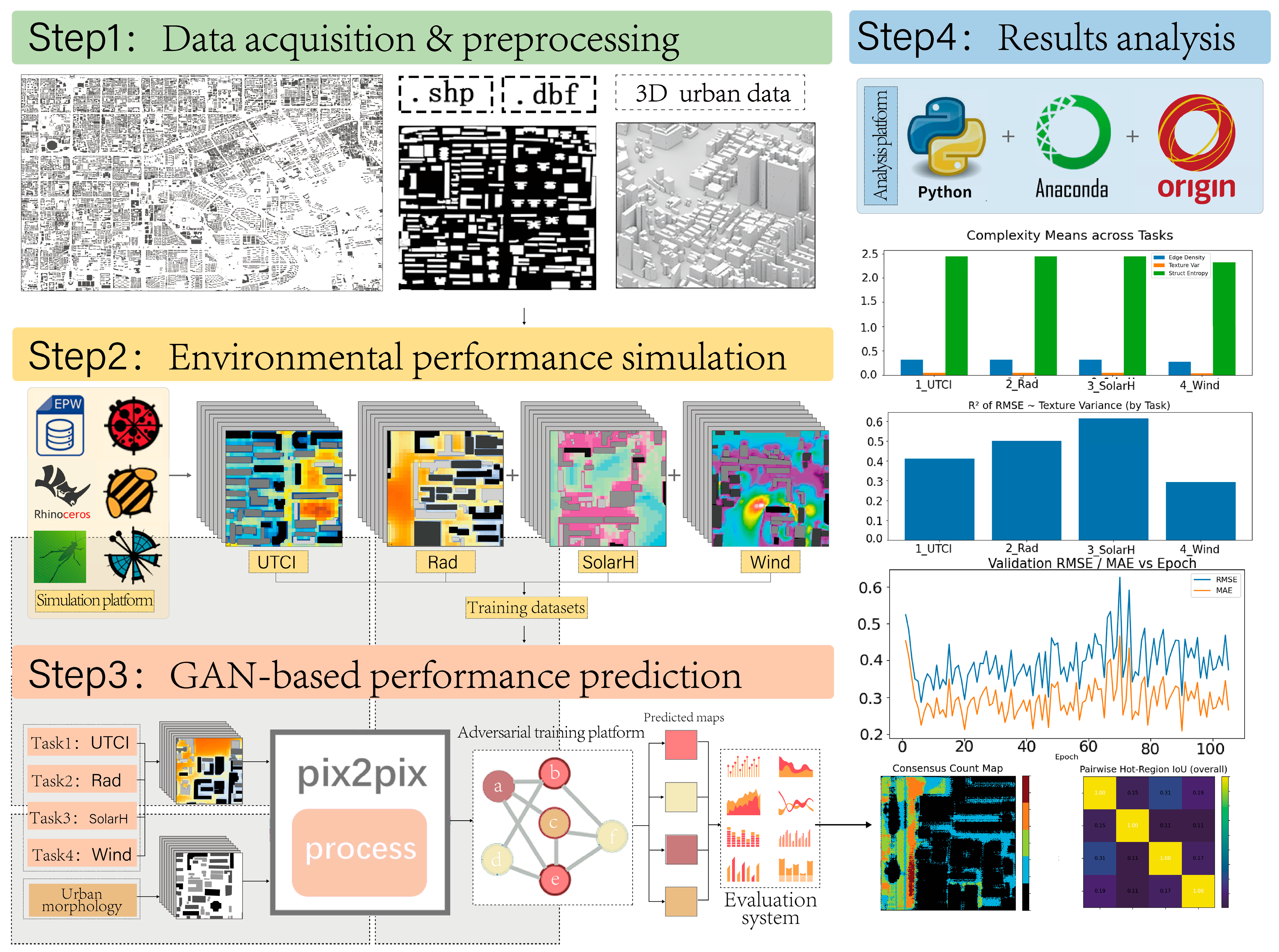
A “unified input–multi-target output” workflow is proposed for predicting urban environmental performance, spanning four stages: data preparation, physical simulation, adversarial learning, and result evaluation (Figure 1). At the block scale, a standardised urban-form raster serves as the input to learn and predict four targets—UTCI, annual solar irradiation (Rad), sunshine duration (SolarH), and near-ground wind field (Wind). A multi-dimensional evaluation of accuracy, efficiency, and spatial semantic consistency is then performed. Step 1 (data preprocessing): Integrate building/road/green-space layers and 3D models, perform alignment and cleaning, and rasterize them into a single-channel urban-form image as the unified input for all four tasks. The outputs are normalised 2D/3D-form data and aligned raster images. Step 2 (performance simulation): Under the unified form and an EPW meteorological driver, generate ground truth maps for UTCI/Rad/SolarH/Wind, align and normalise them to form input–label pairs, and construct training/validation/test datasets for the four tasks. Step 3 (adversarial prediction): Train four single-task models independently using pix2pix (U-Net generator + PatchGAN discriminator), and record efficiency metrics including total runtime, per-epoch time, and best/plateau epochs. The outputs are prediction maps, training logs, and model weights. Step 4 (integrated evaluation): Assess performance using RMSE/MAE/PSNR/SSIM (pixel level), HIR/IoU_hot/IoU_cold/EOR (structural/regional), and cross-task IoU/synergy–conflict/consensus count, and analyse the complexity–error relationship and learnability differences via edge density, texture variance, and structural entropy, yielding quantitative metrics and visualised findings.
Figure 1.
Study framework and overall pipeline. Colors and letters in the figure are used for visual guidance only; detailed explanations of each step are provided in the main text.
Rationale for using a single-channel morphology raster: A unified single-channel morphology raster (buildings–ground mask) is deliberately adopted as the input for all four tasks to keep the representation minimal and strictly comparable across targets. This design avoids heterogeneous priors introduced by multi-layer tensors (e.g., height, vegetation, land-use) and aligns with the objective of isolating learnability differences that arise from the physical nature of the targets rather than from differences in the input richness or encoding schemes.
3.2. Study Area and Data Preparation
3.2.1. Study Area
The study area is the central urban district of Xi’an, China, characterised by a high-density building fabric [26] and representative of a typical northern inland city morphology (Figure 2). Its street network is grid-like and its building layouts are compact, providing a representative high-density block context that facilitates multi-target prediction under a unified urban-form input. Xi’an has a temperate continental monsoon climate, with hot and relatively humid summers, cold and dry winters, and pronounced seasonal and diurnal variability [27]. Xi’an’s Typical Meteorological Year (EPW) is used as the simulation driver and provides hourly dry-bulb temperature, wind speed, global horizontal irradiance (GHI), and other variables, ensuring consistency across the four environmental performance simulations. This EPW corresponds to a monsoon-influenced continental climate with cold winters and hot, relatively dry summers, so wind regimes, solar azimuth ranges, and typical street-canyon aspect ratios are characteristic of Xi’an and similar high-density, grid-pattern, mid-latitude cities. Accordingly, the findings of this study should be interpreted as representative of such high-density, grid-pattern, mid-latitude cities with continental monsoon climates rather than as globally general benchmarks.
Figure 2.
Study area and climate overview. (a) Location of Xi’an within Shaanxi Province and China; (b) extent of the selected high-density urban study area; (c) hourly dry-bulb temperature (°C), wind speed (m/s), and global horizontal radiation (Wh/m2) from the Typical Meteorological Year (EPW), visualized as time–month heatmaps, where warmer colors indicate higher values; (d) average monthly maximum and minimum air temperatures.
3.2.2. Physical Simulation of the Four Environmental Performance Targets
Under a unified urban-form input and the same meteorological driver, Ladybug Tools was used to simulate the four targets and to generate ground truth raster maps as supervised learning labels (Figure 3) [28,29,30]. All simulations adopted Xi’an’s Typical Meteorological Year (EPW) as boundary conditions. Specifically, Rad and SolarH were accumulated over the full Typical Meteorological Year to obtain annual totals, whereas UTCI and Wind were extracted for a representative peak summer hour (14:00 local time on the hottest design day), reflecting the critical period for outdoor thermal comfort and ventilation design. Outputs were strictly co-registered to the input morphology with matched resolution. For training convenience, each task was statistically normalised during training, while preserving physical units for interpretation and inverse rescaling.
Figure 3.
Simulation examples of the four environmental performance targets. Rad and SolarH represent annual aggregates over the Typical Meteorological Year, whereas UTCI and Wind correspond to a representative peak summer hour (14:00 on the hottest design day). For each target, colors indicate the magnitude of the corresponding variable, with warmer colors representing higher values and cooler colors representing lower values.
The Universal Thermal Climate Index (UTCI) maps meteorological variables to thermal stress via a human heat balance model [31]. Using dry-bulb temperature, relative humidity, wind speed, and mean radiant temperature as inputs, UTCI was computed per pixel from standard formulas and spatially aligned to the block-scale ground grid. For this study, the focus is on the peak summer design period; therefore, the UTCI field at 14:00 on the hottest representative day is used as the supervisory label.
Annual solar irradiation (Rad) was obtained by integrating shortwave components over the solar course with geometric occlusion to yield yearly ground irradiance [32]. In this process, direct, diffuse, and reflected components with shadowing/occlusion are computed considering building masses and solar position, and the per-pixel annual total on the horizontal or near-ground plane (Wh/m2) is accumulated.
Sunshine duration (SolarH) was derived by accumulating hourly binary shadow tests with a direct irradiance threshold [33]. Based on solar altitude/azimuth and occlusion tests, the annual hours meeting the “directly sunlit” condition (h/yr) are counted for each pixel, forming a continuous sunshine duration field.
The near-ground wind field (Wind) was computed via morphology-constrained flow solutions to obtain mean wind speed distributions. Given the prevailing wind direction and boundary wind speed, simplified steady-state flow simulations were performed to obtain these fields (parametric/simplified CFD) [34,35,36,37] and project the results onto the ground grid to characterise ventilation corridors and recirculation zones. To be consistent with the UTCI target, the simulated wind field corresponds to the same peak summer hour described above, and the output unit is m/s.
Rationale for the four output targets: Taken together, these four outputs represent the main physical drivers of outdoor environmental performance at the block scale. Annual Rad and SolarH capture long-term solar accessibility, which constrains daylighting potential, passive gains, and shading strategies, whereas peak summer UTCI and Wind describe the most critical hours for outdoor thermal stress and natural ventilation along streets and courtyards. Urban design decisions such as the placement of corridors, courtyards, and canopies typically depend on these indicators simultaneously, which is why they are treated as a coherent multi-target set in this study.
The four outputs were standardised into model-readable label rasters and paired one-to-one with the input morphology to form four task-specific datasets. To mitigate scale differences, each task was statistically normalised during training, while original physical units were retained for post hoc interpretation and inverse rescaling.
Justification of the simulation toolchain: Ladybug Tools was selected for UTCI, Rad, and SolarH because it offers validated radiative and thermal models, open source implementation and direct compatibility with EPW files, which facilitates reproducibility. For the wind field, simplified steady-state CFD was used to obtain mean near-ground wind speeds under the same EPW-driven boundary conditions, striking a balance between physical realism and computational tractability over more than 2100 samples. Using this homogeneous toolchain ensures that differences in learnability are not confounded by inconsistent simulation settings across targets. It should be noted that these numerically simulated fields act as a surrogate ground truth under unified conditions, and their inherent uncertainties—particularly the reduced precision of simplified CFD wind fields compared with high-fidelity LES or on-site measurements—likely introduce additional label noise for the Wind task. These limitations and their implications for learnability are discussed in Section 5.3.
3.3. Model Architecture and Training Pipeline
3.3.1. Model Architecture and Modelling Strategy (pix2pix)
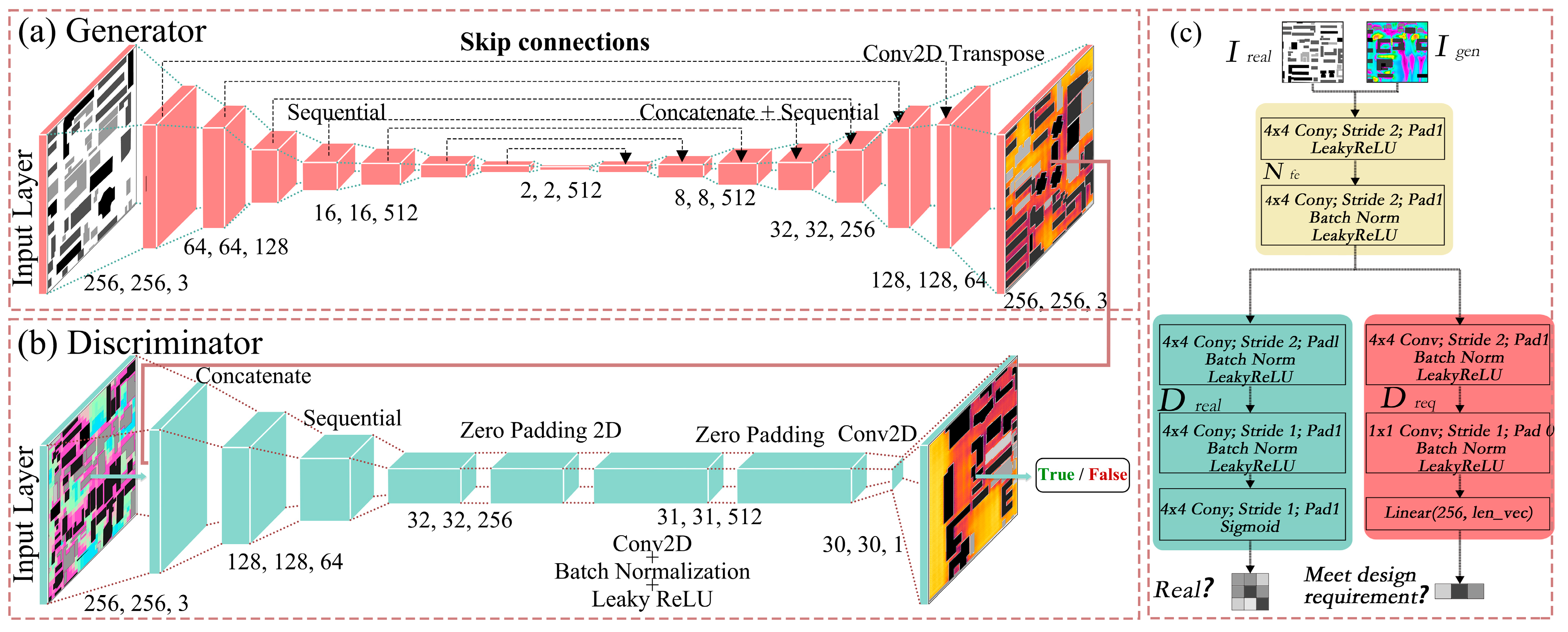
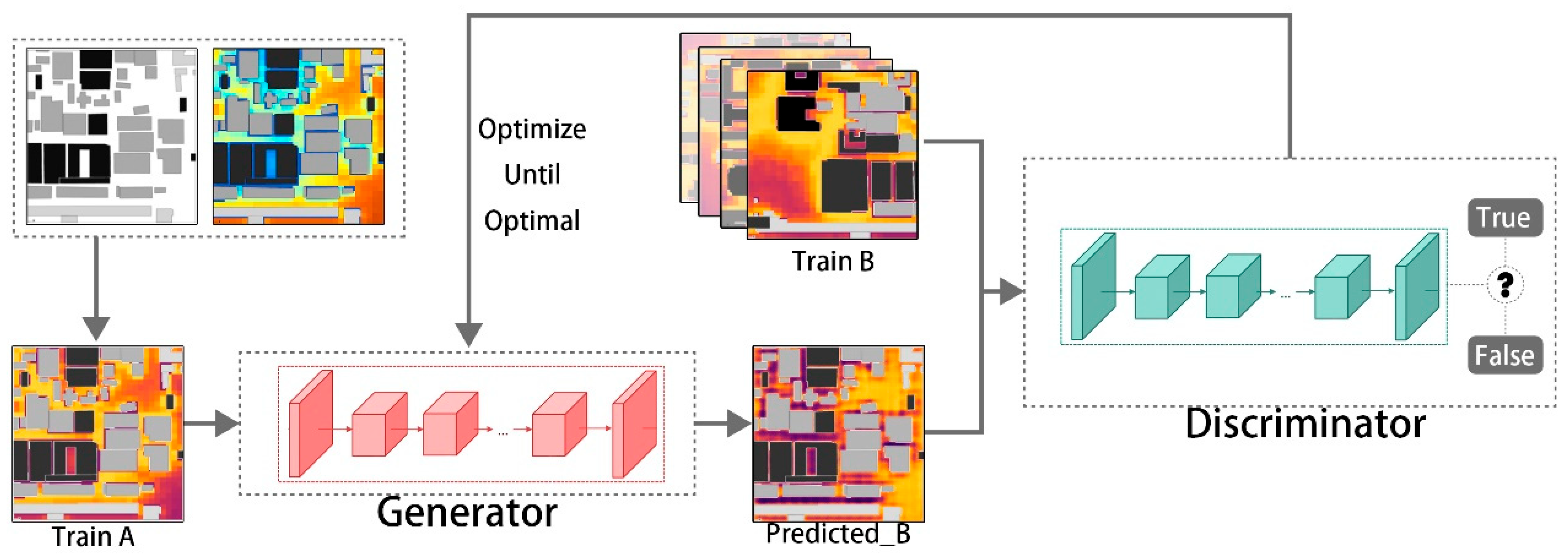
A pix2pix conditional adversarial framework is adopted that models the mapping from urban-form images to environmental performance maps as an end-to-end image-to-image translation task. The generator G is a skip-connected U-Net encoder–decoder that preserves details and reconstructs large-scale continuous fields. The discriminator D is a 70 × 70 PatchGAN that judges realism over local receptive fields and reinforces texture and edge consistency (Figure 4 and Figure 5). The objective combines an adversarial term with a pixel consistency term to jointly secure perceptual fidelity and numerical accuracy. Specifically, L = LGAN(G,D) + λLL1(G), where λ is set relatively high to suppress artefacts and improve numerical approximation. A shared L1 objective across all four targets is deliberately adopted to keep the optimisation scale unified. This design allows differences in performance to be attributed primarily to the physical nature of the targets rather than to heterogeneous loss weighting. The four targets (UTCI, Rad, SolarH, Wind) are implemented as four independent pix2pix models with identical architectures and training settings. Multi-task variants with shared backbones were considered but not adopted, because preliminary trials and prior studies indicated that partially conflicting physical mechanisms (e.g., smooth radiative and sunshine fields versus highly turbulent wind fields) can cause gradient interference and degrade task-specific accuracy. Using four symmetric single-task models, therefore, provides a cleaner basis for comparing learnability and convergence behaviour across targets.
Figure 4.
Architecture of the pix2pix model. (a) Generator network based on a U-Net architecture with encoder–decoder structure and skip connections, where feature maps from the encoder are concatenated with corresponding decoder layers to preserve spatial details. (b) PatchGAN discriminator architecture, which classifies local image patches as real or fake to enforce high-frequency realism. (c) Detailed structure of the discriminator blocks, illustrating convolutional layers, batch normalization, activation functions, and the final decision layers. Different colors indicate different functional modules (e.g., convolutional blocks, normalization layers, and activation layers), dashed boxes denote network components or stages, and arrows indicate the data flow during forward propagation.
Figure 5.
Training workflow of the pix2pix framework. The generator learns a mapping from the input urban morphology (A) to the target environmental performance map (B), while the PatchGAN discriminator evaluates whether the generated output is realistic when paired with the input. Colored blocks represent different network components, dashed boxes indicate training stages, and arrows denote the iterative data flow between the generator and discriminator during adversarial training.
3.3.2. Data Preprocessing and Sample Construction
Each pair consists of a standardised urban-form input and a pixel-aligned task label, rasterized under a common spatial reference. Raw vector/3D features are projection-harmonised, topologically cleaned, and encoded to produce a single-channel form image; simulation outputs for the four targets are resampled to a common resolution and size, then normalised to [0, 1] (or standardised) to remove unit-scale disparities. This normalisation is not intended to equalise the physical impact of errors across tasks, but rather to provide a common numerical scale that enables fair cross-target comparison under the same training objective. Each target is normalised using min–max scaling computed on the training set so that all labels lie within [0, 1] while preserving their monotonic ordering, and the same affine mapping is applied to the validation and test sets. This procedure stabilises optimisation, keeps the relative distribution and ranking of each physical field intact, and places all outputs on a comparable numerical scale for joint analysis. Datasets are split in a spatially disjoint manner and augmented lightly to enhance generalisation. All data are partitioned into 70%/15%/15% training/validation/test splits, with block-level de-duplication to prevent leakage, and spatially adjacent tiles are avoided across splits wherever possible so that no identical or nearly identical morphology patches appear in more than one subset. Tiles are fixed at 256 × 256, and augmentations such as translation and random cropping are applied; the four tasks share identical input specifications and tiling masks, differing only in labels.
3.3.3. Training Parameters and Hyperparameter Settings
Optimisation follows standard pix2pix practice, with early stopping to balance convergence and efficiency. Adam (β1 = 0.5, β2 = 0.999) is used with an initial learning rate of 2 × 10⁻⁴, linearly decayed in later epochs; a small batch size is chosen to fit GPU memory; discriminator and generator learning rates are set either equal or with TTUR to stabilise adversarial training. Training logs record both efficiency and accuracy metrics. The checkpoint with the best validation SSIM or lowest RMSE is retained, and total runtime, average per-epoch time, best epoch, and plateau epoch are recorded. At test time, RMSE, MAE, PSNR, SSIM, and structural/regional metrics (HIR, IoU, EOR) are reported for subsequent comparative analysis (Figure 5).
3.3.4. Hyperparameter Standardisation Across Targets
To ensure that differences in performance and learnability can be attributed to the physical nature of the targets rather than to model configuration, all four pix2pix instances share the same architecture and training hyperparameters. Table 1 summarises the common settings. The generator is a U-Net with eight encoder–decoder stages and skip connections, and the discriminator is a 70 × 70 PatchGAN; all models use 256 × 256 inputs, Adam optimisation (β1 = 0.5, β2 = 0.999), an initial learning rate of 2 × 10⁻⁴ with linear decay, a batch size of 1, and an L1 weight λ chosen to emphasise numerical accuracy while suppressing artefacts. Data splits (70%/15%/15% train/validation/test), the normalisation scheme, and the augmentation strategy are also kept identical across UTCI, Rad, SolarH, and Wind. No task-specific hyperparameters are tuned separately; only emergent quantities such as the best epoch, plateau epoch, and total runtime differ between tasks and are reported in the Results section.
Table 1.
Shared model and training hyperparameters for the four pix2pix surrogates.
3.4. Comparison and Evaluation of Predictive Performance
In Step 4, the predictive performance of the four GAN surrogates is compared and evaluated under a unified protocol. The analysis is organised into five complementary components that together capture pixel-level fidelity, structural consistency, training efficiency, cross-task interactions, and semantic learnability.
- (1)
- Pixel-level metrics
For each task and for each test image, pixel-wise consistency between prediction ŷ and ground truth y is quantified using standard regression and image quality metrics. The root mean square error (RMSE) is computed as follows:
where N is the number of pixels in the block. In addition, the mean absolute error (MAE), peak signal-to-noise ratio (PSNR), and structural similarity index (SSIM) are reported to characterise intensity bias, dynamic-range compression, and local texture similarity, respectively. A lower RMSE/MAE and higher PSNR/SSIM indicate better performance. For each task, the distributions of these metrics over the test set are summarised using medians and dispersion, and between-task comparisons are carried out when relevant.
- (2)
- Structural consistency metrics
Pixel-level metrics do not explicitly capture the shape and extent of patterns that are critical for design decisions, such as hotspots, shaded pockets, or ventilation corridors. To assess structural behaviour, binary maps for “hot” and “cold” regions are derived by thresholding each field at fixed quantiles (e.g., top/bottom 15%), and the intersection over union (IoU_hot, IoU_cold) between the predicted and ground truth regions is computed. In addition, Canny edges are extracted on both maps and the edge overlap ratio (EOR) is measured as the fraction of overlapping edge pixels. Together, these metrics quantify whether the model preserves the spatial structure and boundaries of critical regions, rather than merely matching pixel values.
- (3)
- Training efficiency and stability
To characterise efficiency, the total training time, average time per epoch, the epoch at which the best validation SSIM is reached, and the length of the subsequent performance plateau are recorded. Loss curve convergence and volatility are also inspected to judge the trade-off between speed and stability, allowing comparisons not only of final accuracy but also of how quickly and reliably each task can be learned.
- (4)
- Cross-task synergy and semantic learnability
To investigate whether tasks share learnable patterns, cross-task synergy maps are constructed by intersecting correctly predicted hot (or cold) regions across pairs of targets and computing their IoU. High synergy indicates that similar morphological cues support multiple targets, whereas low synergy highlights conflicts or decoupling, as in the case of wind. In parallel, learnability is assessed by relating prediction errors to the semantic complexity of the input morphology. For each block, texture variance, edge density, and entropy are computed on the morphology raster and then correlated with RMSE at the block level, with R2 values reported. A high R2 between texture variance and RMSE for radiation tasks suggests that complex patterns are harder to learn, whereas a very low R2 for wind indicates that turbulence-related variability dominates over purely morphological complexity.
- (5)
- Visualisation and reproducibility
The above analyses are summarised using a minimally sufficient figure set: absolute error maps, examples of hot/cold-region overlap, boxplots of the main metrics, and synergy/conflict matrices. All statistics are computed on the held-out test set. For each metric (RMSE, MAE, PSNR, SSIM, IoU), both median values and 5th–95th percentile ranges are reported to quantify variability across different block morphologies, and fixed random seeds are used to support reproducibility. Variability across the test set is visualised through the dispersion ranges in the boxplots, which serve as empirical uncertainty bands for design-oriented interpretation.These bands characterise uncertainty across spatial samples for a single trained model; variance due to repeated training runs with different initialisations is not separately estimated in this study and is identified as future work (Section 5.3).
4. Results and Analysis
4.1. Training Process and Efficiency Analysis
4.1.1. Training Time and Resource Consumption
All four tasks were trained under identical hardware and batch settings, yet the total time exhibited a clear hierarchy: Wind was the longest, followed by SolarH and UTCI, whereas Rad was the shortest (Figure 6a). The per-epoch time ranged from 5.3 to 5.9 s/epoch and was nearly identical across tasks, indicating similar per-step computational costs; hence, the overall time was governed primarily by how many epochs each model required (Figure 6b). The number of epochs needed to reach the best performance (through peak validation SSIM) was approximately Wind ≈ 145, SolarH ≈ 91, UTCI ≈ 65, and Rad ≈ 28, mirroring the total time ranking and showing that efficiency differences arise mainly from convergence epochs rather than per-epoch computation (Figure 6c). Plateau epochs (Δ < 1 × 10⁻⁴, patience = 5) were about Wind ≈ 21, Rad ≈ 18, UTCI ≈ 14, and SolarH ≈ 13, indicating that Wind requires longer late-stage exploration, Rad is the next longest, and SolarH and UTCI stabilise more quickly (Figure 6d). Under identical resources, Rad is the most economical to train and Wind the most costly. Because per-epoch times are nearly equal, early stopping, learning-rate decay, and patience tuning can directly curb the total training time and compute usage (Figure 6).
Figure 6.
Training time and convergence efficiency across tasks. (a) Total training time; (b) average epoch time; (c) best epoch from validation SSIM; (d) plateau epoch (Δ = 1 × 10⁻⁴, patience = 5).
4.1.2. Convergence Speed and Training Stability
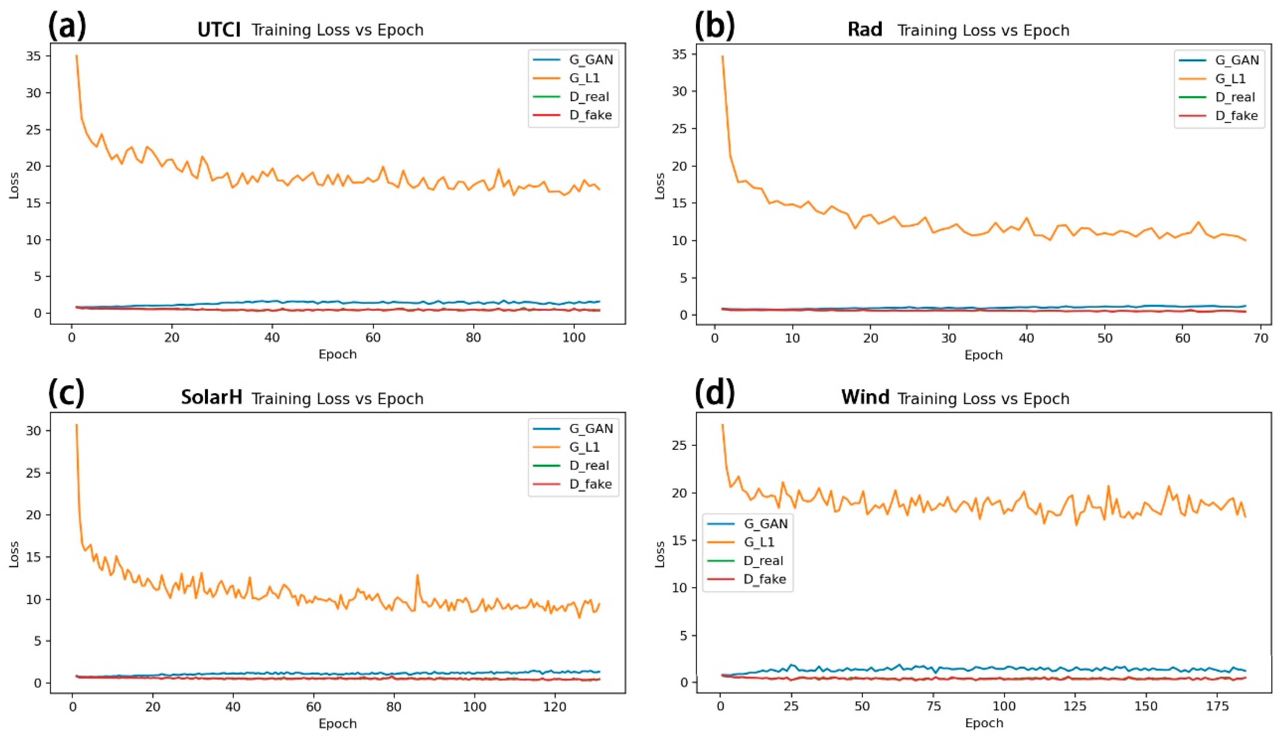
All four tasks exhibit a “rapid drop → plateau stabilization” convergence pattern, yet they differ markedly in stability and speed (Figure 7a–d). Rad converges the fastest with the smoothest curves: the pixel reconstruction loss GL1 drops quickly and fluctuates at a low level, while the adversarial term GGAN and discriminator losses (Dreal, Dfake) remain low and stable without signs of divergence (Figure 7b). SolarH trains longer yet remains overall stable: GL1 declines gradually before reaching a low plateau; occasional small spikes recede quickly; and the two discriminator branches have comparable magnitudes, indicating a balanced adversarial game (Figure 7c). UTCI shows a moderate convergence with acceptable stability: GL1 decreases markedly in early epochs and plateaus slightly higher than Rad/SolarH thereafter; adversarial and discriminator losses undulate mildly without imbalance (Figure 7a). Wind oscillates noticeably and converges the slowest: G_L1 stays elevated for a prolonged period with larger fluctuations, and G_GAN varies with higher amplitude and frequency, suggesting a greater sensitivity to adversarial training and a harder learning problem (Figure 7d). Under identical settings, Rad is the fastest and most stable, SolarH is stable but requires more epochs, UTCI is intermediate, and Wind is difficult to learn with pronounced oscillations (Figure 7). This matches the earlier ranking by total time and best epoch, indicating that efficiency differences are driven primarily by convergence difficulties rather than per-epoch computational costs. In particular, the unstable and slow convergence of Wind reflects the underlying turbulence and recirculation in the CFD-like labels, which make the adversarial game more sensitive and the mapping inherently harder to learn.
Figure 7.
Training losses versus epoch for the four pix2pix models. (a) UTCI; (b) Rad; (c) SolarH; (d) Wind. Each subplot shows the generator adversarial loss (G_GAN), generator reconstruction loss (G_L1), and discriminator losses on real and fake pairs over the training epochs.
4.2. Multi-Target Prediction Results and Overall Performance
4.2.1. Prediction–Ground Truth Comparison and Structural Reconstruction
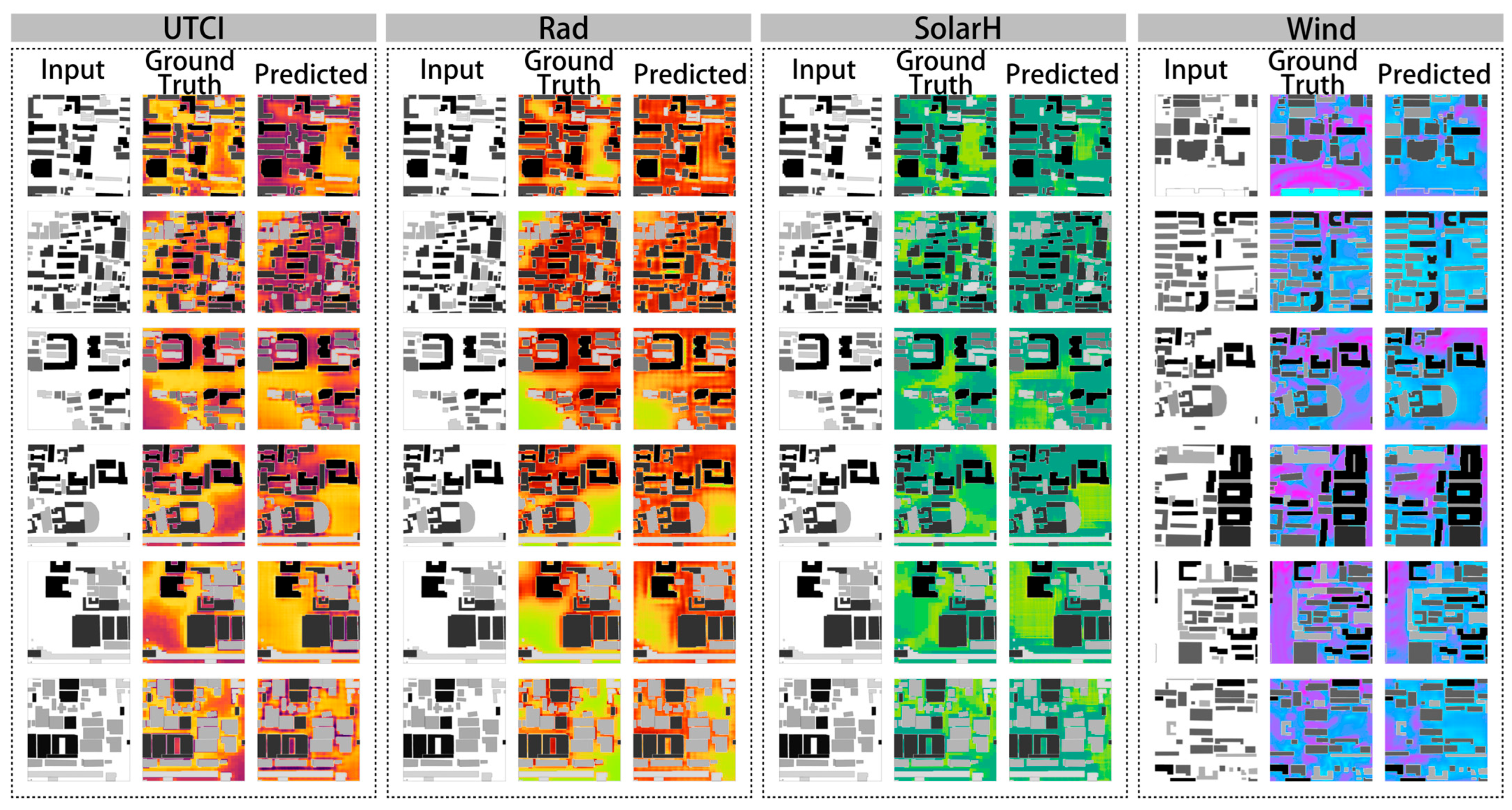
Overall, the model reconstructs continuous fields across all four tasks while preserving key spatial semantics, particularly the strength–weakness banding along street orientations, open spaces, and occlusion belts. The three columns show input form–ground truth–prediction; the predicted maps align with the ground truth in large-scale gradients and in building-shadow/sunshine striping, indicating that end-to-end learning has captured the dominant “form-to-performance” relationship (Figure 8). Structural reconstruction is most stable for radiation (Rad) and sunshine duration (SolarH), followed by thermal comfort (UTCI), whereas the wind field (Wind) is relatively weaker. In the Rad/SolarH panels, the high–low patterns at building projections, street corridors, and courtyard openings align well with the ground truth, with only slight smoothing in a few narrow alleys; the strong–weak partitioning in UTCI is broadly correct, though mild over-smoothing appears near boundaries. Wind reproduces the outlines of dominant corridors and recirculation zones, but it misses details and introduces artefacts at corners, narrow passages, and local backflows. These areas are typically associated with turbulence, flow separation, and small recirculation cells, which adversarial models find difficult to reconstruct from a single morphology channel. Typical errors concentrate in narrow gaps and sharp edges, manifesting as edge distortion, local over-smoothing, or small artefacts. These observations accord with the subsequent analyses of the edge overlap ratio (EOR) and hot/cold-region overlap, suggesting that stronger edge/gradient constraints or multi-scale feature alignment in adversarial training may further improve structural fidelity.
Figure 8.
Prediction–ground truth comparison and structural fidelity across four tasks. Colors indicate relative magnitudes of each environmental variable within the same task, with warmer and cooler tones representing higher and lower values, respectively.
4.2.2. Visual Perceptual Quality Assessment
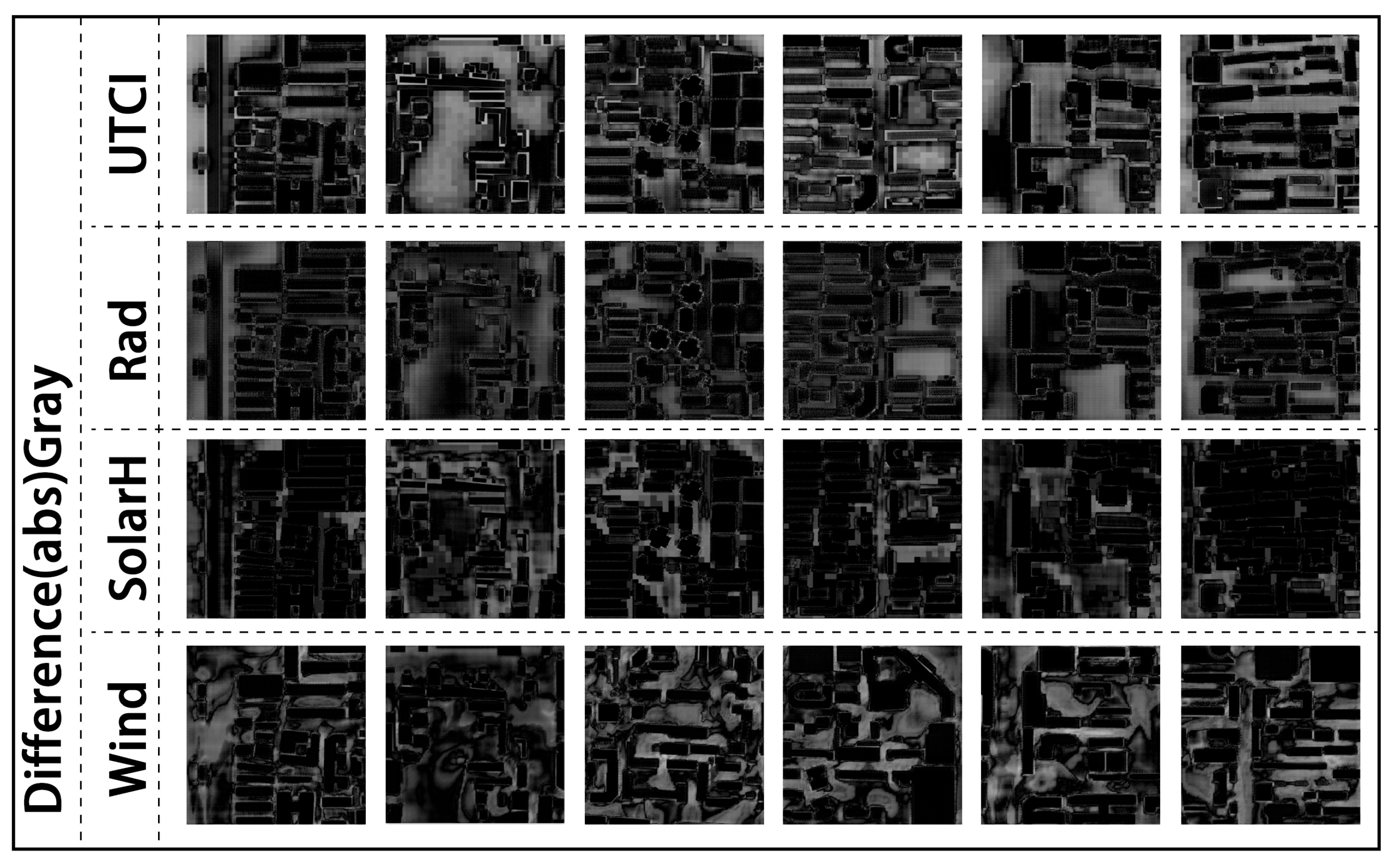
The absolute error maps reveal the visual error distribution and its structural correlation across the four tasks: Rad and SolarH exhibit the smallest errors, UTCI is intermediate, and Wind is comparatively larger. Each map encodes per-pixel absolute differences in grayscale—black denotes low error and white denotes high error; rows correspond to tasks and columns to different samples, enabling side-by-side comparisons (Figure 9). For Rad/SolarH, the background is generally dark, with only thin bright bands along building edges and narrow alleys, indicating the good reconstruction of large-scale gradients and occlusion striping, with errors concentrated near geometric discontinuities. UTCI shows a moderate error intensity, with a slight diffusion around boundaries, suggesting that banding in the thermal comfort field is captured, yet boundary over-smoothing remains the primary issue. Wind exhibits a mottled error pattern that spreads along corners, ventilation corridors, and local recirculation zones. This behaviour is consistent with the wind field’s high nonstationarity and local turbulence, and it implies that pixel consistency constraints alone are insufficient to capture fine-scale details in zones of flow separation and aerodynamic instability. Overall, the absolute error maps corroborate the structural reconstruction findings: Rad/SolarH achieve a higher visual quality, UTCI is usable but boundary-smooth, and Wind shows pronounced errors in complex flow regions. These observations provide an intuitive support for subsequent structural consistency metrics, including the edge overlap ratio (EOR) and hot/cold-region IoU.
Figure 9.
Grayscale absolute error maps (black = low error, white = high error).
4.2.3. Quantitative Comparison of Accuracy Metrics
Across the four metrics, the results consistently show that SolarH and Rad perform best, UTCI is intermediate, and Wind is relatively the weakest (Figure 10). The task-wise means of the RMSE indicate the lowest error for SolarH, followed by Rad, with Wind and UTCI higher; in other words, pixel-level errors are smaller for SolarH/Rad (Figure 10a). PSNR agrees with the RMSE: SolarH is the highest, Rad follows, and Wind/UTCI are lower, indicating a better signal-to-noise ratio for the former two (Figure 10b). The mean SSIM likewise yields the order SolarH ≳ Rad > UTCI > Wind (Figure 10c), and SSIM boxplots further show that SolarH has the highest median with moderate dispersion; Rad is slightly lower yet stable; UTCI is intermediate with a few low outliers; and Wind has the lowest median and a more dispersed distribution (Figure 10d). Overall, for the objective of “lower error and higher similarity/SNR,” SolarH and Rad dominate both numerically and structurally; UTCI is usable, but boundary over-smoothing is reflected in SSIM and PSNR, whereas Wind underperforms in both pixel errors and structural consistency. This ordering accords with the earlier visual comparisons and convergence stability analysis. It should also be noted that, although all targets are trained under a unified normalised objective, the same relative error corresponds to different physical magnitudes (e.g., several tenths of a degree Celsius for UTCI versus a few hundredths of m/s for Wind), which designers should take into account when interpreting the metrics.
Figure 10.
Overall accuracy comparison by task. (a) RMSE, (b) PSNR, and (c) SSIM. Bars show the median values computed over the test set. (d) SSIM distribution across test samples shown as boxplots, where the central line indicates the median, the box denotes the interquartile range, whiskers represent the data range excluding outliers, circles denote outliers, and the triangle marker indicates the mean value. The dispersion ranges illustrate variability across the test set and serve as an approximate confidence interval for interpreting model stability.
4.3. Mechanistic Explanation of Learnability Differences
4.3.1. Definition of Semantic Complexity Metrics
“Learnability difficulty” is characterised using three image-level semantic complexity metrics: edge density, texture variance, and structural entropy. Edge density is the proportion of edge pixels per unit area (ratio after Sobel/Canny detection), indicating contour fragmentation and the frequency of structural turns. Texture variance is the image-wide mean of sliding-window grayscale variance, representing the magnitude of local undulations/texture. Structural entropy is the entropy of the grayscale histogram (or the mean of block-wise entropies), indicating distributional uncertainty/mixing. These metrics are computed for each image, aggregated within each task, and later related to error to explain learnability differences across targets. In terms of means, the four tasks show a comparable complexity; Wind is slightly lower in edge/texture, while structural entropy is nearly identical (Figure 11). Specifically, edge density ranges from 0.27 to 0.32, with Wind slightly lower and UTCI/SolarH/Rad similar; texture variance is small overall yet still differentiates tasks, being slightly lower for Wind and comparable among the others; structural entropy is about 2.4–2.5, with minimal cross-task differences. This suggests that the data preparation preserved cross-task morphological comparability, and that subsequent differences in the complexity–error relationship are more likely to reflect task-specific physics and label noise rather than sample distribution bias.
Figure 11.
Mean semantic complexity across tasks.
4.3.2. Analysis of the Complexity–Error Relationship
Texture variance explains the error substantially better than edge density and shows a stable ranking across tasks. The R2 bar charts indicate that edge density → RMSE has a weak explanatory power overall (all < 0.07): Rad ≈ 0.07, Wind ≈ 0.02, UTCI ≈ 0.02, and SolarH ≈ 0.01 (Figure 12a). By contrast, texture variance → RMSE increases markedly and yields a clear ordering: SolarH ≈ 0.62 > Rad ≈ 0.45 > UTCI ≈ 0.30 ≫ Wind ≈ 0.05 (Figure 12b). These results suggest that the more a task is dominated by continuous-field characteristics, the better its errors can be explained by texture undulations; conversely, wind fields affected by turbulence and local extremes are poorly captured by simple texture statistics. Specifically, the high R2 for SolarH and Rad indicates that their errors are governed primarily by large-scale texture and gradients; UTCI is of intermediate strength, combining continuous banding with local perturbations; and the very low R2 for Wind points to physical complexity and label nonstationarity as primary causes beyond what edge/texture statistics can explain, consistent with the turbulent and recirculating nature of urban wind fields. Within this “complexity → error” framework, texture variance emerges as a more effective indicator of learnability, whereas edge count is not decisive—consistent with earlier conclusions on convergence and visual quality. These relationships are interpreted as descriptive indicators of learnability rather than as causal links: they summarise how physical complexity and label noise jointly modulate the difficulty of fitting each target under the unified training protocol, without implying that any single complexity metric directly causes the observed errors.
Figure 12.
Error explained by complexity metrics across tasks. (a) Coefficient of determination (R2) between edge density and RMSE for each task. (b) Coefficient of determination (R2) between texture variance and RMSE for each task.
4.4. Spatial Structural Consistency and Semantic Recognition
Hot-region overlap maps provide an intuitive test of prediction–ground truth consistency in “hotspot” space: Rad and SolarH achieve the highest hit rates, UTCI is intermediate, and Wind is comparatively weaker (Figure 13). Colours are encoded as follows: yellow denotes hits (Pred ∩ GT), cyan denotes misses (GT-only), red denotes false alarms (Pred-only), and black marks non-hot regions; rows correspond to tasks and columns to different samples, enabling side-by-side comparisons. For Rad/SolarH, yellow hits appear as contiguous blocks primarily along building shadow bands, street orientations, and open space boundaries, whereas cyan/red misses/false alarms are mostly thin, narrow strips. This indicates that the model preserves large-scale banding and block-like hotspots well, with limitations concentrated at geometric discontinuities and narrow gaps. UTCI shows a moderate consistency: hotspot regions are correctly located, but boundary transitions are wide, producing thin cyan/red fringes adjacent to hit bands—consistent with earlier observations of slightly smoothed boundaries. Wind exhibits the lowest consistency: hits are fragmented and cyan/red artefacts increase markedly at corners, narrow passages, and recirculation zones, suggesting that local nonstationarity and turbulence around corners and separation zones make hotspot detection more sensitive and predictions more prone to spatial offsets. Overall, the overlap maps corroborate semantic preservation at the structural level—Rad, SolarH > UTCI > Wind—in agreement with pixel/perceptual metrics and providing intuitive support for subsequent quantitative measures such as IoU/HIR and EOR.
Figure 13.
Hot-region overlap between prediction and ground truth. Yellow indicates hits (Pred ∩ GT), cyan indicates misses (GT-only), red indicates false alarms (Pred-only), and black denotes non-hot regions in both prediction and ground truth.
4.5. Cross-Target Synergy and Semantic Conflict Identification
4.5.1. Synergistic Structure Identification: Analysis of Spatial Overlap Maps
Cross-task overlays reveal spatial structures of joint response within urban blocks: synergistic zones distribute continuously along open corridors and stable occlusion bands, whereas conflict points concentrate at geometric discontinuities and narrow corner gaps (Figure 14a). In the synergy/conflict map, yellow denotes multi-task agreement (synergy), red indicates opposing responses across tasks (conflict), and black marks non-focus regions. Most samples are dominated by extensive yellow synergy regions, indicating that the four targets share a common spatial orientation along principal bands and blocky structures; localised red spots and lines are frequent at building corners, narrow canyons, and flow-separation zones, suggesting local inconsistencies driven by differing physical mechanisms. The consensus strength map further quantifies how many tasks agree and corroborates the morphology seen in the synergy map. In the consensus count map (0–4), warmer colours indicate a higher agreement: counts of 3–4 typically trace street centrelines and stable shadow/irradiance zones, whereas counts of 0–1 cluster in geometrically complex areas and wind disturbance zones (Figure 14b). This indicates that cross-task consensus structures have a clear spatial directionality and delineate potential priority zones for multi-target consistency analysis, providing qualitative support for subsequent quantitative IoU and consistency metrics.
Figure 14.
Cross-task synergy/conflict maps and consensus count maps. (a) Synergy/conflict: yellow = synergy, red = conflict, black = background; (b) consensus count: 0–4; cool = low (0–1), warm = high (3–4).
4.5.2. Construction of Synergy Metrics and Quantitative Evaluation
Cross-task synergy is quantified using pairwise IoU over hot and cold regions: the synergy in hot regions is generally low, whereas cold-region agreement is markedly higher among UTCI–Rad–SolarH, with Wind showing the weakest consistency with any other target (Figure 15a,b). In hot regions, UTCI–SolarH attains the highest IoU (~0.31), while most other pairs fall within 0.11–0.19, indicating that extreme highs are strongly impacted by local geometry and differing physical mechanisms, which hinder cross-task alignment (Figure 15a). In cold regions, UTCI–SolarH and UTCI–Rad reach approximately 0.70/0.65, and Rad–SolarH about 0.64, all substantially exceeding their hot-region counterparts; by contrast, Wind pairs at only ~0.18–0.19 with any task, evidencing clear decoupling (Figure 15b). Overall, cross-task synergy follows a robust pattern—Cold > Hot and UTCI–Rad–SolarH > Wind—suggesting that background areas dominated by smooth radiative and thermal gradients more readily achieve consensus, whereas extreme highs and wind fields are controlled by highly local mechanisms (e.g., corner vortices, canyon jets, recirculation bubbles) and nonstationarity. These results provide quantitative support for subsequent multi-objective design trade-offs. In particular, the low hot-region IoU for Wind is consistent with the physics of urban flow: extreme velocities tend to concentrate near corners, sharp bends, and recirculation pockets, where turbulence, flow separation, and aerodynamic instabilities make peak locations highly sensitive to small geometric changes, so that even qualitatively correct patterns yield fragmented overlap at the hotspot level.
Figure 15.
Pairwise IoU matrices across tasks. (a) Pairwise Intersection-over-Union (IoU) for hot regions, showing cross-task agreement in extreme high-value areas. (b) Pairwise Intersection-over-Union (IoU) for cold regions, indicating cross-task agreement in background or low-value areas.In both panels, colour encodes the mean IoU values over the test set.
5. Discussion
5.1. Comparison with Alternative Predictive Models
Although pix2pix was selected as the baseline model in this study, it is useful to position the method relative to other predictive approaches. Traditional regression or CNN-based predictors often achieve a low computational cost but struggle to preserve spatial boundaries, local gradients, and high–low region structures, which are essential for environmental fields such as solar irradiation, thermal comfort, or wind. CycleGAN models, while powerful for unpaired translation, introduce additional ambiguity in label alignment and generally exhibit a weaker numerical faithfulness when ground truth rasters are available.
Multi-task architectures could, in principle, share representations across targets; however, preliminary trials and previous studies suggest that conflicting physical mechanisms (e.g., continuous radiative fields versus turbulent wind fields) can lead to gradient interference and degraded task-specific accuracy. In contrast, pix2pix offers a stable compromise: it is a fully supervised, paired translation framework whose geometry-aware U-Net architecture preserves spatial semantics while maintaining reproducible training behaviour.
This comparison clarifies why pix2pix is adopted as the baseline under unified inputs: it supports strict cross-target comparability, provides reliable structural reconstruction, ensures reproducible convergence behaviour, and minimises confounding factors related to unpaired learning or multi-task interference. In this way, the methodological positioning helps to contextualise the empirical findings and delineate future directions for hybrid or physics-informed extensions.
5.2. Predictability Hierarchy and Practical Implications
The four targets exhibit a stable ranking in predictability and efficiency: SolarH ≈ Rad > UTCI > Wind. This ordering holds consistently across four dimensions: pixel accuracy, structural consistency, cross-task synergy, and training efficiency. Texture variance explains errors better than edge density, cross-task synergy follows a “Cold > Hot” pattern, and Wind is clearly decoupled from the other targets.
These differences arise from the physical properties and statistical characteristics of the fields. SolarH and Rad are dominated by large-scale continuous gradients and stable occlusion bands, leading to a higher texture learnability, faster convergence, and more stable structures. UTCI involves multi-factor coupling; while still continuous, its boundaries tend to be over-smoothed. Wind is driven by turbulence and local extremes, is highly nonstationary, and is more sensitive to adversarial training, yielding mottled errors and unstable structures.
Under unified conditions, this study fills the gap in cross-performance comparison and structural/synergy evaluation. Beyond prior GAN-based fast approximations for wind or radiation, UTCI, Rad, SolarH, and Wind are evaluated in parallel under the same inputs and protocol, extending assessment from the pixel level to structural and synergistic levels and providing verifiable evidence on reliability differences and applicability bounds. Methodologically and practically, this study contributes a reusable pixel–structure–synergy–learnability baseline and clear guidance: the toolkit can serve as a general workflow for “learning to replace simulation”. At the design scheme stage, SolarH/Rad GAN surrogates are more robust, whereas Wind should be paired with physics consistency constraints or hybrid paradigms (e.g., GAN + CFD/PINN) to enhance boundary and detail credibility. Cross-task synergy/conflict maps and consensus counts can directly support multi-objective trade-offs and sensitivity analysis by indicating where multiple targets agree or conflict in space.
5.3. Limitations and Future Work
The dataset currently covers a single city and climate, and therefore merits cross-city and cross-climate validation to examine whether the observed hierarchy (SolarH ≈ Rad > UTCI > Wind) holds under different wind regimes, urban morphologies and radiative contexts, especially in maritime, tropical, and high-latitude climates where these quantities may differ substantially from the Xi’an setting.
The labels depend entirely on numerical simulations (Ladybug Tools for UTCI, Rad, and SolarH and simplified steady-state CFD for Wind). These fields are internally consistent under unified EPW-driven boundary conditions, but they cannot fully replace the experimental validation of real urban microclimates. In future work, they should be complemented by field or wind-tunnel measurements—for example, drone-based campaigns and fixed-sensor networks—to better characterise label noise and absolute accuracy, especially for the wind field. For the Wind target in particular, the use of simplified steady-state CFD with coarse turbulence modelling is expected to introduce additional label noise and the smoothing of fine-scale structures, which may partly explain the lower apparent learnability and weaker structural performance observed for this task.
In terms of modelling paradigms, the present study focuses on single-task pix2pix surrogates. This invites extensions to multi-task and multi-scale or attention-based architectures, as well as hybrid or physics-informed models (e.g., GANs combined with CFD or PINNs), with explicit uncertainty reporting at both pixel and region levels. Such developments would help quantify prediction confidence, particularly in critical hotspots and ventilation corridors, and are further elaborated in the technical roadmap outlined in Section 5.4. In addition, uncertainty is currently characterised only through dispersion across the held-out test set (median and 5th–95th percentile ranges); systematic estimates of run-to-run variance under repeated training with different random initialisations are not yet included and will be incorporated in future work to provide more complete uncertainty quantification for key performance metrics. Overall, under unified conditions, this work provides systematic evidence and clear bounds for multi-target GAN prediction, offering an actionable path for engineering deployment and methodological expansion.
5.4. Technical Roadmap for Improving Wind Target Surrogates
The Wind field is the most challenging target in terms of accuracy, structural consistency, and convergence stability. Building on the above limitations, a technical roadmap can be outlined along three complementary axes: enriched inputs, tailored architectures, and embedded physics.
First, additional input variables can be incorporated to reduce ambiguity when inferring wind from morphology. Beyond the single-channel footprint mask used in this study, future datasets could include directional roughness or frontal-area indices, surface roughness length, land-use type, and simple turbulence indicators (e.g., coarse recirculation or shear masks). Such descriptors would help distinguish geometries with similar footprints but different aerodynamic behaviour and thus improve generalisation to unseen urban patterns.
Second, at the model level, architectures with explicit multi-scale and anisotropic receptive fields are promising for Wind. Examples include U-Net variants with dilated convolutions or pyramid pooling to capture wide canyon structures, and hybrid CNN–transformer encoders that represent long-range alignments along corridors and open spaces. Decoder modules with gradient- or edge-aware regularisation can further help preserve sharp velocity changes at corners and along jets.
Third, simplified physics mechanisms can be introduced as soft constraints within the learning process. Physics-inspired losses may penalise divergence and encourage approximate mass conservation, limit unphysical overshoots via gradient-based regularisation, or enforce consistency with coarse steady-state flow patterns. Coarse CFD fields or turbulence indicators can serve as auxiliary input channels or teacher signals, while PINN-like formulations can embed simplified momentum or continuity equations directly into the loss.
Together, these three directions form a concise roadmap for future work on the Wind target, complementing the unified baseline established in this study and guiding subsequent developments in data acquisition, model design, and physics integration.
6. Conclusions
Under unified inputs and a consistent evaluation protocol, this study systematically compares the predictive performance of pix2pix across four urban environmental targets (UTCI, Rad, SolarH, Wind) for a high-density Xi’an case. The work establishes a closed-loop assessment spanning pixel–structure/region–cross-task synergy–learnability–efficiency and provides reproducible timing and epoch statistics on more than 2100 block-scale pairs.
Within the monsoon-type climate and grid-pattern morphology considered here, multidimensional findings consistently indicate a stable ranking: SolarH ≈ Rad > UTCI > Wind. This ranking is supported consistently by RMSE/PSNR/SSIM, absolute error visualisations, edge overlap, hot/cold-region IoU, and synergy/conflict and consensus count metrics. In efficiency terms, per-epoch times are similar, whereas best/plateau epochs differ markedly, indicating that the total training time is governed more by convergence difficulty than by raw computational cost.
The learnability mechanism reveals that continuous fields are easier to learn, whereas wind fields are harder. Texture variance explains error far better than edge density—being highest for SolarH and Rad, moderate for UTCI, and minimal for Wind—which implies that large-scale continuous gradients and stable occlusion bands are effectively captured by adversarial learning, while wind fields dominated by turbulence and local extremes are poorly constrained by simple texture statistics.
Methodologically and practically, this study delineates clear applicability bounds and usage guidance. The proposed evaluation toolkit serves as a general baseline for “learning in lieu of simulation.” For conceptual and early design stages, SolarH and Rad surrogates are well suited for rapid iteration, enabling designers to screen alternative block layouts, corridor orientations, and courtyard configurations with second-level feedback on solar access and long-term irradiation potential. UTCI surrogates can be used as an intermediate filter to flag areas of potential thermal stress, but final comfort assessment should be complemented by full atmospheric and microclimatic frameworks, especially in critical seasons. Wind surrogates are most appropriate as qualitative or pre-screening tools to highlight ventilation corridors and potential risk zones, and should be paired with physics consistency constraints or hybrid paradigms (e.g., GAN+CFD/PINN) to avoid critical errors in sensitive areas such as plazas, schoolyards, or pedestrian canyons. Cross-task synergy/conflict maps and consensus counts can directly support multi-objective trade-offs and sensitivity analysis by identifying where multiple targets agree or conflict spatially.
These practical recommendations are consistent with city-scale thermal comfort mapping frameworks such as the WRF–UCM–SOLWEIG chain proposed by Ding et al. [38], where solar and net radiation are used to support the quick initial screening of design alternatives, while UTCI and wind-related comfort are evaluated through more rigorous, full-physics simulations. This alignment reinforces the complexity hierarchy observed in the present study and underscores the importance of tailoring surrogate usage to the physical nature and dynamical complexity of each environmental metric.
This study remains limited in its data breadth, climatic scope, and modelling paradigm, but the improvement path is clear. The current findings are conditioned on a single city and climate and on numerically generated labels; the observed hierarchy of learnability should therefore not be assumed to generalise to maritime, tropical, or high-latitude climates without further testing. Future work will pursue cross-city and cross-climate validation, introduce field and wind-tunnel calibration—such as drone-based campaigns and fixed-sensor networks for the Wind target—extend to multi-task shared backbones and multi-scale/attention or perceptual–boundary joint losses, and further standardise uncertainty and confidence interval reporting to enhance transferability and engineering utility.
From an operational perspective, the unified urban-form input and per-target pix2pix generators can be wrapped as services or plug-ins within parametric design environments (e.g., Rhino/Grasshopper), GIS platforms, or urban sustainability assessment tools. In such workflows, candidate block morphologies can be sent to the surrogates and return multi-target environmental fields, synergy/conflict maps, and basic confidence indicators within seconds, providing a practical bridge between fast data-driven prediction and more detailed physics-based simulation in real-world planning processes.
Author Contributions
Conceptualization, C.W. and S.W.; methodology, S.W. and C.W.; software, S.W., C.W., S.R. and W.L.; validation, C.W. and S.R.; formal analysis, S.R.; investigation and data acquisition, W.L., W.Y. and M.Q.; resources, M.Q. and W.Y.; data curation, W.L. and W.Y.; writing—original draft preparation, S.W.; writing—review and editing, C.W.; visualisation, S.W., C.W. and M.Q.; supervision, S.W. All authors have read and agreed to the published version of the manuscript.
Funding
This research received no external funding.
Institutional Review Board Statement
Not applicable.
Informed Consent Statement
Not applicable.
Data Availability Statement
The data presented in this study are available on request from the corresponding author. The data are not publicly available due to privacy.
Conflicts of Interest
Author Mei Qing was employed by Xi’an Qujiang Cultural Finance Holding (Group) Co., Ltd. The company had no role in the design, execution, interpretation, or writing of this study. The remaining authors declare that the research was conducted in the absence of any commercial or financial relationships that could be construed as a potential conflict of interest.
Abbreviations
The following abbreviations are used in this manuscript:
| CFD | Computational Fluid Dynamics |
| EOR | Edge Overlap Ratio |
| EPW | EnergyPlus Weather File |
| GAN | Generative Adversarial Networks |
| GHI | Global Horizontal Irradiance |
| IoU | Intersection Over Union |
| LIME | Local Interpretable Model-Agnostic Explanations |
| LPIPS | Learned Perceptual Image Patch Similarity |
| MAE | Mean Absolute Error |
| PDP | Partial Dependence Plot |
| PINN | Physics-Informed Neural Networks |
| PSNR | Peak Signal-to-Noise Ratio |
| Rad | Annual Global Solar Radiation |
| RMSE | Root Mean Square Error |
| SHAP | Shapley Additive Explanations |
| SolarH | Sunshine Duration |
| SSIM | Structural Similarity Index |
| UTCI | Universal Thermal Climate Index |
References
- Chen, L.; Huang, H.; Yao, D.; Yang, H.; Xu, S.; Liu, S. Construction of Urban Environmental Performance Evaluation System Based on Multivariate System Theory and Comparative Analysis: A Case Study of Chengdu-Chongqing Twin Cities, China. Int. J. Environ. Res. Public Health 2023, 20, 4515. [Google Scholar] [CrossRef] [PubMed]
- Peng, Y.; Peng, Z.; Feng, T.; Zhong, C.; Wang, W. Assessing comfort in urban public spaces: A structural equation model involving environmental attitude and perception. Int. J. Environ. Res. Public Health 2021, 18, 1287. [Google Scholar] [CrossRef]
- Huo, H.; Chen, F.; Geng, X.; Tao, J.; Liu, Z.; Zhang, W.; Leng, P. Simulation of the urban space thermal environment based on computational fluid dynamics: A comprehensive review. Sensors 2021, 21, 6898. [Google Scholar] [CrossRef]
- Li, W.; Xu, X.; Yao, J.; Chen, Q.; Sun, Z.; Makvandi, M.; Yuan, P.F. Natural ventilation cooling effectiveness classification for building design addressing climate characteristics. Sci. Rep. 2024, 14, 16168. [Google Scholar] [CrossRef] [PubMed]
- Calzolari, G.; Liu, W. Accelerating Large Eddy Simulations of urban airflow with Generative Adversarial Networks. Build. Environ. 2025, 286, 113622. [Google Scholar] [CrossRef]
- Zheng, L.; Lu, W. Urban micro-scale street thermal comfort prediction using a ‘graph attention network’model. Build. Environ. 2024, 262, 111780. [Google Scholar] [CrossRef]
- Luo, Z.; Huang, W. FloorplanGAN: Vector residential floorplan adversarial generation. Autom. Constr. 2022, 142, 104470. [Google Scholar] [CrossRef]
- Wang, L.; Liu, J.; Zeng, Y.; Cheng, G.; Hu, H.; Hu, J.; Huang, X. Automated building layout generation using deep learning and graph algorithms. Autom. Constr. 2023, 154, 105036. [Google Scholar] [CrossRef]
- Tan, C.; Zhong, X. A rapid wind velocity prediction method in built environment based on CycleGAN model. In Proceedings of the International Conference on Computational Design and Robotic Fabrication, Shanghai, China, 25–26 June 2022; Springer Nature: Singapore, 2022; pp. 253–262. [Google Scholar]
- Li, J.; Guo, F.; Chen, H. A study on urban block design strategies for improving pedestrian-level wind conditions: CFD-based optimization and generative adversarial networks. Energy Build. 2024, 304, 113863. [Google Scholar] [CrossRef]
- Quan, S.J. Urban-GAN: An artificial intelligence-aided computation system for plural urban design. Environ. Plan. B Urban Anal. City Sci. 2022, 49, 2500–2515. [Google Scholar] [CrossRef]
- Sun, C.; Zhou, Y.; Han, Y. Automatic generation of architecture facade for historical urban renovation using generative adversarial network. Build. Environ. 2022, 212, 108781. [Google Scholar] [CrossRef]
- Mokhtar, S.; Sojka, A.; Davila, C.C. Conditional generative adversarial networks for pedestrian wind flow approximation. In Proceedings of the 11th Annual Symposium on Simulation for Architecture and Urban Design, Virtual, 25–27 May 2020; pp. 1–8. [Google Scholar]
- Milla-Val, J.; Montañés, C.; Fueyo, N. Adversarial image-to-image model to obtain highly detailed wind fields from mesoscale simulations in urban environments. Build. Environ. 2024, 266, 112123. [Google Scholar] [CrossRef]
- Lu, Y.; Li, X.; Wu, S.; Wang, Y.; Qiu, W.; Chen, D.; Li, Y. SolarGAN for Meso-Level Solar Radiation Prediction at the Urban Scale: A Case Study in Boston. Remote Sens. 2024, 16, 4524. [Google Scholar] [CrossRef]
- Zhang, Y.; Schlueter, A.; Waibel, C. SolarGAN: Synthetic annual solar irradiance time series on urban building facades via Deep Generative Networks. Energy AI 2023, 12, 100223. [Google Scholar] [CrossRef]
- Huang, C.; Zhang, G.; Yao, J.; Wang, X.; Calautit, J.K.; Zhao, C.; An, N.; Peng, X. Accelerated environmental performance-driven urban design with generative adversarial network. Build. Environ. 2022, 224, 109575. [Google Scholar] [CrossRef]
- Zhu, Y.; Wang, Y.; Li, J.; Song, Q.; Chen, D.; Qiu, W. BikeshareGAN: Predicting dockless bike-sharing demand based on satellite image. J. Transp. Geogr. 2025, 126, 104245. [Google Scholar] [CrossRef]
- Wu, A.N.; Biljecki, F. InstantCITY: Synthesising morphologically accurate geospatial data for urban form analysis, transfer, and quality control. ISPRS J. Photogramm. Remote Sens. 2023, 195, 90–104. [Google Scholar] [CrossRef]
- He, Q.; Li, Z.; Gao, W.; Chen, H.; Wu, X.; Cheng, X.; Lin, B. Predictive models for daylight performance of general floorplans based on CNN and GAN: A proof-of-concept study. Build. Environ. 2021, 206, 108346. [Google Scholar] [CrossRef]
- Cheng, B.; Girshick, R.; Dollár, P.; Berg, A.C.; Kirillov, A. Boundary IoU: Improving object-centric image segmentation evaluation. In Proceedings of the IEEE/CVF Conference on Computer Vision and Pattern Recognition, Virtual, 19–25 June 2021; pp. 15334–15342. [Google Scholar]
- Zhang, R.; Isola, P.; Efros, A.A.; Shechtman, E.; Wang, O. The unreasonable effectiveness of deep features as a perceptual metric. In Proceedings of the IEEE Conference on Computer Vision and Pattern Recognition, Salt Lake City, UT, USA, 18–23 June 2018; pp. 586–595. [Google Scholar]
- Ostmeier, S.; Axelrod, B.; Isensee, F.; Bertels, J.; Mlynash, M.; Christensen, S.; Lansberg, M.G.; Albers, G.W.; Sheth, R.; Verhaaren, B.F.; et al. USE-Evaluator: Performance metrics for medical image segmentation models supervised by uncertain, small or empty reference annotations in neuroimaging. Med. Image Anal. 2023, 90, 102927. [Google Scholar] [CrossRef]
- Darvishvand, L.; Kamkari, B.; Huang, M.J.; Hewitt, N.J. A systematic review of explainable artificial intelligence in urban building energy modeling: Methods, applications, and future directions. Sustain. Cities Soc. 2025, 128, 106492. [Google Scholar] [CrossRef]
- Córdoba Hernández, R.; Camerin, F. Assessment of ecological capacity for urban planning and improving resilience in the European framework: An approach based on the Spanish case. Cuad. Investig. Geográfica 2023, 49, 119–142. [Google Scholar] [CrossRef]
- Ren, W.; Zhao, J.; Ma, X.; Wang, X. Analysis of the spatial differentiation and scale effects of the three-dimensional architectural landscape in Xi’an, China. PLoS ONE 2021, 16, e0261846. [Google Scholar] [CrossRef]
- Liu, J.; Li, J.; Gao, Z.; Yang, M.; Qin, K.; Yang, X. Ecosystem services insights into water resources management in China: A case of Xi’an city. Int. J. Environ. Res. Public Health 2016, 13, 1169. [Google Scholar] [CrossRef]
- Salamone, F.; Belussi, L.; Currò, C.; Danza, L.; Ghellere, M.; Guazzi, G.; Lenzi, B.; Megale, V.; Meroni, I. Integrated method for personal thermal comfort assessment and optimization through users’ feedback, IoT and machine learning: A case study. Sensors 2018, 18, 1602. [Google Scholar] [CrossRef]
- Chen, T.; Tan, L. Multiobjective optimization of external shading for west facing university dormitories in Kunming considering solar radiation and daylighting. Sci. Rep. 2025, 15, 21876. [Google Scholar] [CrossRef]
- Wu, Z.; Xu, Y.; Wang, Z. Multi-objective optimization of energy, view, daylight and thermal comfort for building’s fenestration and shading system in hot-humid climates. PLoS ONE 2025, 20, e0325290. [Google Scholar] [CrossRef] [PubMed]
- Burgstall, A.; Casanueva, A.; Kotlarski, S.; Schwierz, C. Heat warnings in Switzerland: Reassessing the choice of the current heat stress index. Int. J. Environ. Res. Public Health 2019, 16, 2684. [Google Scholar] [CrossRef] [PubMed]
- Alkhatib, H.; Norton, B.; O’Sullivan, D.T.J.; Lemarchand, P. Calibration of solar pyranometers for accurate solar irradiance measurements: A data set from the pre-and post-calibration process. Data Brief 2025, 59, 111402. [Google Scholar] [CrossRef]
- Hidalgo-García, D.; Rezapouraghdam, H. Variability of heat stress using the UrbClim climate model in the city of Seville (Spain): Mitigation proposal. Environ. Monit. Assess. 2023, 195, 1164. [Google Scholar] [CrossRef]
- Guo, M.; Cao, Y.; Wang, P.; Zhao, L.; Li, Y. A generation and recommendation algorithm for high-rise building layout. South Archit. 2022, 9, 96–106. (In Chinese) [Google Scholar] [CrossRef]
- Yang, H.; Zhao, N.; Yang, Q.; Xu, H. Preliminary study on generative design of green high-rise office buildings based on multi-objective optimization. In Proceedings of the National Symposium on Digital Technology Teaching and Research in Architecture (China), Wuhan, China, 18–19 September 2021. (In Chinese). [Google Scholar]
- Chen, G.; Rong, L.; Zhang, G. Unsteady-state CFD simulations on the impacts of urban geometry on outdoor thermal comfort within idealized building arrays. Sustain. Cities Soc. 2021, 74, 103187. [Google Scholar] [CrossRef]
- Kastner, P.; Dogan, T. Eddy3D: A toolkit for decoupled outdoor thermal comfort simulations in urban areas. Build. Environ. 2022, 212, 108639. [Google Scholar] [CrossRef]
- Ding, X.; Zhao, Y.; Strebel, D.; Fan, Y.; Ge, J.; Carmeliet, J. A WRF-UCM-SOLWEIG framework for mapping thermal comfort and quantifying urban climate drivers: Advancing spatial and temporal resolutions at city scale. Sustain. Cities Soc. 2024, 112, 105628. [Google Scholar] [CrossRef]
Disclaimer/Publisher’s Note: The statements, opinions and data contained in all publications are solely those of the individual author(s) and contributor(s) and not of MDPI and/or the editor(s). MDPI and/or the editor(s) disclaim responsibility for any injury to people or property resulting from any ideas, methods, instructions or products referred to in the content. |
© 2025 by the authors. Licensee MDPI, Basel, Switzerland. This article is an open access article distributed under the terms and conditions of the Creative Commons Attribution (CC BY) license (https://creativecommons.org/licenses/by/4.0/).