Assessment of Sensor Data from an Air Quality Monitoring Network—The Need for Machine Learning-Based Recalibration and Its Relevance in Health Impact Analysis of Local Pollution Events

Abstract

Accurate, high-resolution air quality data are crucial for understanding environmental health risks; however, the cost and complexity of maintaining dense, reference-grade monitoring networks remain a significant barrier. This study presents the first city-wide evaluation of next-generation air quality sensors in Zagreb, Croatia, involving 35 sensor locations, one local reference-grade station, and three national reference stations that measure PM₁₀ and NO₂. Sensor performance was evaluated against reference data under various meteorological and temporal conditions. To better understand sensor drift and measurement bias, we developed machine learning (ML) calibration models (XGBoost) using spatiotemporal features, ERA5 meteorological variables, and traffic proxy indicators. The models significantly improved accuracy, reducing the root mean squared error (RMSE) by up to 82%, with the greatest improvements observed during pollution peaks. A rolling Root Mean Square Error (RMSE) approach was introduced to track model degradation over time, revealing that recalibration was typically needed within 1–6 months. Our findings demonstrate that, with proper calibration and maintenance, sensor networks can serve as reliable and scalable tools for urban air quality monitoring, capable of supporting both public health assessments and informed decision-making.

1. Introduction

1.1. The Health Relevance of PM₁₀ and NO₂ Exposure

Accurate, high-resolution monitoring of air quality is essential for understanding the health impacts of environmental pollution. Exposure to pollutants such as particulate matter (PM) and nitrogen dioxide (NO₂) has been connected to a wide range of negative health outcomes, including respiratory and cardiovascular issues, impaired lung development, and increased mortality [1,2,3]. PM refers to a mixture of solid particles and liquid droplets suspended in the air and is typically categorized by size. PM₁₀, for example, consists of particles with diameters of 10 micrometers (µm) or smaller, which are small enough to be inhaled into the upper respiratory tract [3]. These very fine particles, as well as PM_2.5 (particles smaller than 2.5 µm), are health risk indicators that can include dust, pollen, or other aeroallergens, as well as soot, smoke, and various chemical compounds, such as polycyclic aromatic hydrocarbons (PAHs) and heavy metals [4]. Depending on their molecular weight and ambient temperature, PAHs can exist in both the gaseous phase and adsorbed onto particles, with lighter compounds predominantly present in the gaseous phase and heavier ones predominantly bound to particles. They are emitted from both natural and anthropogenic sources, with major urban contributors including traffic emissions (especially from diesel engines, road vehicle tire and brake wear, etc.) [5], industrial activities, construction work [6], and residential heating using gas, biomass, or coal [7,8,9]. Once inhaled, PM_2.5 and PM₁₀ can cause inflammation and oxidative stress in the lungs, potentially triggering or exacerbating respiratory and cardiovascular diseases [10]. Long-term exposure has been associated with chronic bronchitis, reduced lung function, and increased risk of heart attacks and strokes [11,12]. Fine particles (those with aerodynamic diameters of 2.5 µm or smaller) can also penetrate deeper into the lungs and, in some cases, enter the bloodstream, posing systemic health risks. In contrast, ultrafine particles, which are smaller than 0.1 µm, can also enter the bloodstream, thereby posing additional systemic health risks [13].

NO₂ is a gaseous air pollutant primarily produced during the combustion of fossil fuels [14]. It is a common byproduct of vehicle engines, power plants, and heating systems. In urban settings, road traffic is typically the dominant source, particularly from diesel vehicles [15]. NO₂ contributes to the formation of ground-level ozone and secondary PM, but it is also directly harmful to human health [16]. Short-term exposure to elevated levels of NO₂ can cause airway irritation, coughing, and reduced lung function, particularly in vulnerable groups such as children, the elderly, and individuals with asthma or chronic obstructive pulmonary disease [17,18]. Long-term exposure is associated with increased susceptibility to respiratory infections and may lead to the development of asthma in children [19]. Given the high exposure levels in urban areas, PM₁₀ and NO₂ are among the primary indicators in air quality regulations, monitoring frameworks, and health impact assessments.

1.2. The Need for High-Resolution Air Quality Monitoring

Despite the importance of detailed air pollution data, the high cost and logistical complexity of deploying and maintaining dense networks of reference-grade monitoring stations make it difficult for many cities to meet growing monitoring demands. As a result, large-scale air quality assessments often rely on model-based estimates, which may lack the spatial resolution needed to capture local pollution hotspots. To address this issue, updated European air quality legislation requires an increased number of measurement points, more diverse pollutant indicators, and higher spatial coverage, thereby placing pressure on local authorities to expand their monitoring capacity [20]. The regulatory framework for air quality management in Europe is defined by the EU Ambient Air Quality Directive (EC 2008/50) [21], which sets significantly lower limit and target values for pollutants, including PM_2.5, PM₁₀, and NO₂. The Directive also establishes data quality objectives, measurement requirements, and minimum numbers of monitoring sites based on population and pollution levels. Furthermore, the Directive places particular emphasis on public transparency, the development of user-friendly tools for the general population, and the communication of risk in a manner tailored to vulnerable subgroups.

In recent years, low-cost sensor networks integrated with environmental monitoring systems have emerged as a scalable and flexible solution, enabling cities to gather large volumes of data at a fraction of the cost of traditional stations [22,23]. Moreover, low-cost sensors are extending their capabilities beyond ambient air quality and can also measure indoor air quality [24], providing an opportunity to assess human exposure more comprehensively. However, these sensors can be susceptible to measurement drift, environmental interference, and data inaccuracies. To ensure data quality, periodic recalibration is necessary, often every few months, depending on the pollutant type, environmental conditions, and sensor design [25,26,27]. Regardless of periodic recalibration, sensor data are required for modeling, useful for spatiotemporal monitoring of air quality data, and valuable for health impact assessments.

Machine learning (ML) methods have become increasingly popular for calibrating sensor data due to their ability to model complex, non-linear relationships and incorporate multiple environmental factors [28]. By leveraging meteorological data, temporal features, and proxy variables for traffic and emissions, ML models can significantly reduce measurement error and improve alignment with reference-grade observations. Moreover, adaptive calibration strategies, such as tracking the rolling Root Mean Square Error (RMSE) over time, enable the detection of sensor drift and help determine when recalibration is necessary. Despite these advances, many cities have yet to implement such approaches on a large scale.

Several recent studies have demonstrated that air quality sensor networks, when properly calibrated, can provide valuable and reliable data in addition to that of reference-grade monitors [29,30,31]. In cities like London, Oxford, and Antwerp, researchers have deployed networks of optical or electrochemical sensors and compared them to co-located reference stations. Using ML algorithms such as Random Forest [32] and XGBoost [33], they achieved substantial improvements in accuracy, reporting increases in R² values above 0.75 for NO_2, PM_10, and PM_2.5, as well as reductions in mean absolute error by 37–94% after calibration [23,28]. The calibration frequency depends on the sensor type and local environmental conditions. Still, most studies recommend recalibration every 3 to 6 months, with PM sensors typically requiring more frequent calibration and equivalence with the referral method due to the possible impacts of air temperature (due to the electrical conductivity of oxide materials in sensors), high humidity (temporary effect due to hygroscopicity), and particle composition changes [22,26]. This need for more frequent recalibration aligns with findings from the EU level [34] and municipal deployments, such as the “Zagreb Eco map” (https://ekokartazagreb.stampar.hr/, accessed on 29 September 2025), where monthly recalibration and significant added capacities by the research community are part of maintaining accuracy. In this context, ML offers several advantages for more efficient sensor calibration: it captures non-linear relationships between sensor signals and true pollutant concentrations, integrates diverse inputs such as meteorology and traffic proxies, and supports dynamic recalibration strategies by tracking rolling error metrics, including RMSE. Beyond calibration, ML is increasingly used for anomaly or major event detection [35], transfer learning [29], short-term pollution forecasting, and identifying pollution sources [30], making it a central tool for building reliable, scalable air quality monitoring systems.

In Zagreb, a dense network of sensors has recently been deployed across the city. Quality control tests and equivalence tests between national and local measuring stations, as well as between the local HQ Stampar measuring station and the city sensor system, are carried out regularly by national and local stakeholders in accordance with legislative requirements. To use HQ Stampar as a reference (“orientir”) station for the city sensor system, continuous monitoring is ensured through monthly quality validation of sensor system. Additionally, in line with legal and accreditation framework requirements, during the period from March 2024 to February 2025, an equivalence test was conducted comparing PM₁₀ and PM_2.5 values between the HQ Stampar station and the local city reference station using correlation with gravimetric results. The equivalence test confirmed that, with the application of correction factors, PM₁₀ and PM_2.5 values from HQ Stampar ensure data quality within the required measurement uncertainty of <25%. A positive equivalence test of the HQ Stampar station as the reference station for the sensor system, together with monthly comparability checks of the sensor system, contributes to continuous and efficient monitoring and calibration of sensor system data. Still, until now, no comprehensive evaluation of their performance, calibration needs, local event monitoring, or long-term stability has been published. A recent study [31] compared low-cost AQMesh sensors with reference stations in Zagreb but did not apply ML calibration or assess recalibration intervals, underscoring the need for our extended city-wide approach based on ML and rolling RMSE.

This study presents the first city-wide assessment of sensor data from an air quality sensor network in Zagreb, comparing their performance with that of national reference stations for PM₁₀ and NO₂. Furthermore, we visually assess their performance on monitoring local changes to support event detection. The calibration procedures utilize novel approaches, expanding calibration strategies with atmospheric observations. To understand this, this work also evaluates their sensitivity to environmental conditions, applies ML calibration models, and establishes a framework for continuous monitoring and recalibration. This work supports the broader aim of enabling scalable, reliable, and regulation-compliant urban air quality monitoring.

2. Materials and Methods

This study was conducted in Zagreb, the capital of Croatia, with a population exceeding 800,000 residents and a complex urban morphology comprising dense residential zones and major transportation corridors [36]. As one of the most densely populated cities in Croatia, Zagreb experiences elevated concentrations of PM and NO₂, especially during winter, largely due to traffic emissions, residential heating, adverse meteorological conditions, and cross-border issues.

To assess the potential of sensors for urban air quality monitoring, a dense network of 35 sensor units was deployed across different city districts, co-financed by the EU regional development, research, and innovation fund (Figure 1).

The sensor system used in this study was the AirQ Outdoor platform, developed by Smart Sense (Zagreb, Croatia), representing the pilot version of the company’s current Sensees Environment Monitoring System solution (available at: https://mysensees.com/, accessed on 8 November 2025). For measuring PM₁₀ concentrations, an optical particle counter based on laser light scattering was used, while electrochemical sensors were employed for NO₂ detection. Sensor lifetime features for optical particle counters maintain stable performance for 24–36 months, whereas electrochemical gas sensors (such as those used for NO₂) exhibit a shorter operational lifetime of 12–24 months, depending on environmental exposure and pollutant load. Therefore, routine recalibration and periodic performance checks were implemented to mitigate long-term drift. Sensors showing signal degradation were replaced according to the manufacturer’s and operator’s quality-assurance protocols. Sensor measuring of concentrations at high temporal resolution (hourly) was installed in diverse microenvironments, including streets with heavy traffic load, residential neighborhoods, and suburban areas. Before network deployment, NO₂ sensors were individually calibrated under controlled conditions. For PM₁₀ sensors, a subset of representative units was co-located with a type-approved reference particulate analyzer over an extended period to establish a method of equivalence. Based on this co-location campaign, intra-sensor variability was quantified, and corresponding correction factors were derived and applied to all PM₁₀ sensors to harmonize the measurements. Following deployment, routine operational checks and monthly validation activities were conducted jointly by the sensor network operator and the public health institute expert. These included periodic inspection, data quality control, and recalibration if deviations were detected.

The NO₂ sensor is a high-sensitivity electrochemical (EC) sensor with a measurement range of 0–16,000 ppb, precision of ±5 ppb, and a lower detection limit of 1 ppb. It is factory pre-calibrated and individually characterized for zero offset and sensitivity, with an operational lifetime exceeding 24 months. For PM, the system employs optical particle counters based on laser light scattering to quantify PM₁, PM_2.5, and PM₁₀. The measurement ranges are up to 500 µg/m³ (PM₁), 2000 µg/m³ (PM_2.5), and 5000 µg/m³ (PM₁₀), with a detection limit of 1 µg/m³. These sensors operate reliably within a temperature range of –10 to +50 °C and 0–90% RH. The indicative air quality system is classified as a mid-range solution designed for professional and support applications rather than as a consumer-grade low-cost device.

Sensor placement was coordinated by public health experts in collaboration with local stakeholders and guided by prior pollution maps, population demographics, health indicators, and urban infrastructure characteristics. When selecting micro-locations, the requirements of the Ordinance on Air Quality Monitoring (Official Gazette 72/20) were taken into consideration. Micro-locations for monitoring traffic-related air pollution were selected in collaboration with the Faculty of Transport and Traffic Sciences at the University of Zagreb.

Microscale criteria for sampling points included: unobstructed airflow around the sampling probe inlet (generally free within at least 270°, or 180° for edge-of-settlement locations), without physical obstructions that may influence air movement (typically several meters away from buildings, balconies, vegetation, and other barriers, and at least 0.5 m from the nearest structure), sampling inlet height between 1.5 m (representing the breathing zone) and 4 m above ground level, the sampling probe inlet located in proximity to direct emission sources to avoid sampling undiluted emissions, the sampler exhaust outlet positioned to prevent re-entrainment of exhaust air into the sampling inlet, for traffic-oriented monitoring, sampling probes placed at least 25 m away from major intersections and no more than 10 m from the road curb.

Additional siting considerations included: presence of interfering emission sources, safety and security of equipment and personnel, accessibility for maintenance and calibration, availability of electrical power and telecommunications infrastructure, visibility of the monitoring site within its surroundings, public safety and operator safety, feasibility of co-locating instruments for multiple pollutants, and urban planning and land use constraints. Street lighting poles were identified as optimal installation points for low-cost sensors due to convenient access to electrical power, and formal approval was requested from the competent City Office.

The sensor data were compared against measurements from three high-quality reference monitoring stations operated by the Croatian Meteorological and Hydrological Service (DHMZ), referred to as HQ Zagreb 1, HQ Zagreb 2, and HQ Zagreb 3, as well as the local reference-grade station, Štampar (

Table 1. Measuring stations with their locations (1, 2, 3, 39: reference stations, 4–38: sensors).

Station No.	Measuring Station	Latitude	Longitude
1	HQ ZAGREB_1	45°48′1.77″	15°58′27.28″
2	HQ ZAGREB_2	45°49′25.38″	16°2′8.97″
3	HQ ZAGREB_3	45°45′53.81″	16°0′23.29″
4	Rudes	45°47′50.28″	15°55′2.64″
5	Voltino	45°48′17.28″	15°55′38.28″
6	Tresnjevka/Ljubljanica	45°48′3.96″	15°56′32.28″
7	Podsused	45°49′3.00″	15°50′4.56″
8	Folnegovicevo	45°47′38.04″	16°0′17.64″
9	Borovje	45°47′18.24″	16°0′31.32″
10	Radnicka	45°47′48.15″	16°1′6.41″
11	Savica	45°47′37.32″	15°59′36.60″
12	Tresnjevka/Vukovarska	45°47′57.88″	15°57′43.80″
13	Gajnice	45°49′0.48″	15°52′22.44″
14	Vrbik	45°47′41.93″	15°57′49.10″
15	Donji Grad	45°48′24.88″	15°58′25.53″
16	Centar	45°48′47.16″	15°58′37.56″
17	Tresnjevka/Dom sportova	45°48′28.44″	15°57′6.48″
18	Ravnice	45°49′1.96″	16°2′18.52″
19	NSB	45°47′41.45″	15°58′45.72″
20	Dubrava centar	45°49′45.12″	16°3′ 48.96″
21	Brezovica	45°43′ 26.89″	15°54′27.61″
22	Centar/Marticeva	45°48′47.52″	15°59′34.44″
23	Zitnjak	45°47′40.20″	16°3′2.16″
24	Kruge	45°47′53.67″	15°59′35.32″
25	Botinec	45°45′14.76″	15°56′17.52″
26	Crnomerec	45°48′47.88″	15°56′17.16″
27	Graberje	45°48′47.16″	15°55′49.08″
28	Gornje Vrapce	45°49′57.72″	15°54′14.76″
29	Vinogradska	45°48′55.44″	15°57′11.16″
30	Dubrava/Branimirova	45°49′16.56″	16°3′17.00″
31	Čulinec	45°48′52.92″	16°3′38.52″
32	Novi Jelkovec	45°48′44.64″	16°6′45.36″
33	Volovcica	45°48′27.72″	16°1′3.36″
34	Bukovac	45°50′21.84″	16°0′32.40″
35	Dubrava/Maksimir	45°49′52.68″	16°2′36.96″
36	Gornja Dubrava	45°50′11.40″	16°3′37.08″
37	Dubec	45°49′8.40″	16°0′15.48″
38	Sesvetski Kraljevec	45°49′5.52″	16°10′37.92″
39	HQ Stampar	45°49′54.48″	15°58′49.44″

). These stations represent different pollution contexts: a moderately polluted residential zone, a suburban background site, and an urban center roadside location, respectively. Each sensor unit contained optical PM sensors (based on laser light scattering) and electrochemical NO₂ sensors. Also, PM_2.5, PM₁, SO₂, O₃, CO are monitored. The devices recorded measurements every hour and transmitted data to a central database.

Meteorological parameters, including temperature, relative humidity, wind speed, and surface pressure, were obtained from the ERA5 reanalysis dataset (European Centre for Medium-Range Weather Forecasts, ECMWF). ERA5 provides hourly data at a spatial resolution of 0.1° × 0.1° (~9 km). For each sensor location, the nearest ERA5 grid cell was identified using bilinear interpolation based on latitude and longitude. This ensured spatial alignment between the reanalysis data and ground measurements. The interpolated hourly values were then temporally synchronized with the corresponding hourly sensor records. This procedure was applied to all meteorological variables used in both the sensitivity analysis and calibration models. In addition to these variables, the following meteorological and surface parameters were also included in the analysis: 2 m dewpoint temperature, skin temperature, leaf area index (high vegetation), leaf area index (low vegetation), surface latent heat flux, surface net long-wave (thermal) radiation, evaporation, and surface runoff.

2.1. Data Preparation

The dataset, consisting of hourly measurements from 35 sensors and three national and one local reference stations, underwent several preprocessing steps to enhance model performance and ensure robustness. The data processing followed the steps published previously [31]. First, temporal features (based on timestamps) were encoded using sinusoidal transformations [37]. Specifically, the day of the year and month of the year were transformed using sine and cosine functions to capture seasonal differences in air pollution. Additionally, the Julian day and year were included to account for long-term trends, with Julian day representing a continuously increasing number of days since 1 January 1970. A holiday feature was also added as a binary variable, where 0 indicates a regular day and 1 indicates a holiday.

The period from 27 December to 3 January was classified as a holiday to account for increased pollution associated with New Year’s Eve celebrations and fireworks [38,39]. To approximate traffic-related pollution, a traffic proxy variable was introduced alongside the temporal features, following a polynomial approach [40]. For each hour of the day, the mean pollutant value was calculated from the training set, normalized to a range of −1 to 1, and fitted with a polynomial function. This function was then applied across the entire dataset to simulate daily traffic patterns, since direct traffic data were unavailable. The same method was also used to capture weekly traffic dynamics by the day of the week [40]. Before modelling or sensor calibration, outliers were removed using a 10-h sliding window approach: values falling outside the 0.01 and 0.99 quantiles were filtered out within each window. Rare missing values were handled using an iterative imputer, which models each feature as a function of the others and imputes missing values iteratively using a round-robin strategy. The dataset was then split into two subsets: training and testing. The training set spanned from 1 March 2022 to 25 September 2023. The test set started on 26 September 2023 and continued until the end of the dataset on 28 May 2024. This was also done to evaluate the need for recalibration given longer periods.

2.2. Machine Learning and Statistical Analysis

To analyze pollutant dynamics during rush hours, measuring sites were categorized into three groups: heavy traffic load sites, light traffic load sites, and referent stations. Three sites were picked per category to showcase it. Sites were classified according to the density of surrounding roads and transport lines, along with the overall intensity of traffic activity. Areas experiencing heavy traffic were designated as congestion-prone urban zones, whereas light-traffic sites were found in calmer residential neighborhoods. The heavy traffic load sites included Vrbik, NSB, and Trešnjevka/Vukovarska, while the light traffic load sites were Gajnice, Dubrava/Maksimir, and Čulinec. Additionally, three referent sites, HQ Zagreb 1, 2, and 3, were used.

Hourly measurements of pollutants were extracted for a randomly selected Monday, which was 12 June 2023. To show temporal variations during the morning rush period, only data from 03:00 until 11:00 was selected. This weekday was chosen as it represents a typical working day within the observation period and is not affected by weekend or public holiday traffic anomalies. However, we acknowledge that analysing a single day does not capture differences between weekdays and weekends, nor does it reflect potential afternoon traffic peaks or seasonal variability. Morning rush hours were selected as they represent the most consistent and pronounced traffic-related pollution peak across weekdays, and atmospheric conditions during this period favour pollutant accumulation. To investigate how environmental and temporal factors influence air pollutant concentrations, a two-stage modelling framework comprising a feature sensitivity analysis and ML-based calibration was performed. First, a feature sensitivity analysis was conducted using simple linear regression. Separate models were trained for each sensor location to quantify how different inputs, meteorological parameters (e.g., temperature, humidity, wind speed from ERA5), temporal features (e.g., hour of day, day of week, holidays), and traffic proxy indicators, influence local pollutant concentrations. Input variables were standardized before modelling to allow for direct comparison of regression coefficients across features and stations. Standardization was performed by centering each variable to a mean of zero and scaling it to unit variance.

The idea of this analysis was not predictive performance, but rather interpretability: understanding spatial variability in pollution drivers and the relative importance of each explanatory factor across the sensor network. In addition to sensitivity analysis, Principal Component Analysis (PCA) [41] was applied to explore underlying structures and potential redundancies in the measurement data for both PM₁₀ and NO₂. This approach enabled the identification of potential multicollinearity between stations, the assessment of spatial coherence in pollutant concentrations, and the detection of station-specific behavior. The primary purpose of PCA was to assess the consistency of the sensor network, identify stations with similar or divergent temporal patterns, and detect potential outliers before calibration. In the second stage, ML models to calibrate sensor measurements were developed. The XGBoost (Extreme Gradient Boosting) [33] algorithm was selected due to its ability to model complex, non-linear relationships and interactions among spatiotemporal features. Each model was trained using 5-fold cross-validation, with hyperparameters optimized via Bayesian optimization [42]. The calibration dataset consisted of hourly sensor measurements paired with simultaneously recorded pollutant concentrations from the reference station, which served as the target values in the model. This spatiotemporal calibration strategy allowed the model to correct sensor drift and environmental interference by keeping patterns learned from co-located high-accuracy data. To assess calibration performance, we compared pollutant predictions before and after model correction using the Pearson correlation coefficient and the RMSE. Additionally, we monitored the rolling RMSE over time to detect performance degradation and established thresholds to determine when recalibration was needed.

2.3. Machine Learning-Based Calibration

The calibration process followed a structured, multi-step approach. Hourly pollutant data (PM₁₀ and NO₂), both from sensors and reference stations (1, 2, 3, and 39 operated by DHMZ), formed the core of the training dataset. These data were enriched with engineered temporal features (e.g., sine/cosine encodings of time, holiday markers), meteorological variables from the ERA5 dataset [43,44,45], and proxy indicators of traffic patterns. Sensor-reference pairings were chosen not only based on proximity but also on environmental comparability, considering factors such as traffic exposure, surrounding land use, and microclimatic conditions, including temperature, humidity, and wind direction.

Two sensors were paired with each reference site, resulting in six distinct calibration scenarios. It should be noted that full co-location of sensors directly beside reference-grade monitoring stations was not feasible due to the technical and infrastructural constraints during deployment. Therefore, sensor–reference pairings were established based on spatial proximity and similarity of the local micro-environment rather than identical placement. This approach assumes that nearby sites within comparable micro-environments share similar temporal pollution dynamics, but it cannot eliminate hyperlocal gradients that may cause divergence between sensor and reference values. Consequently, the accuracy metrics presented here should be interpreted as indicators of performance under realistic operational conditions rather than strict equivalence tests. To compensate for the absence of direct co-location, the calibration relied on spatiotemporal patterns by integrating meteorological variables (ERA5), land-use and traffic proxy indicators, and temporal features. This calibration design assumes that the sensors located in comparable urban environments will respond similarly to environmental factors. Therefore, even if exact colocation is not possible, valid calibration relationships can still be established by capturing shared spatiotemporal trends. In the calibration models, the pollutant concentration measured at the reference station was used as the target variable.

In contrast, sensor measurements, meteorological data, temporal features, and land-use variables served as predictors. XGBoost was selected as the calibration algorithm due to its proven ability to capture non-linear and multi-scale relationships, as well as its robustness to noisy input data. Calibration performance was assessed using Pearson correlation coefficients and Mean Squared Error (MSE), both before and after applying the model. In addition, we introduced a rolling RMSE evaluation to monitor performance degradation over time. A reference baseline RMSE was computed on the training set, and recalibration was flagged when the rolling RMSE during the test period exceeded 50% of this baseline. This strategy provided a practical mechanism for determining the temporal stability of the model and guiding the schedule for recalibration.

3. Results

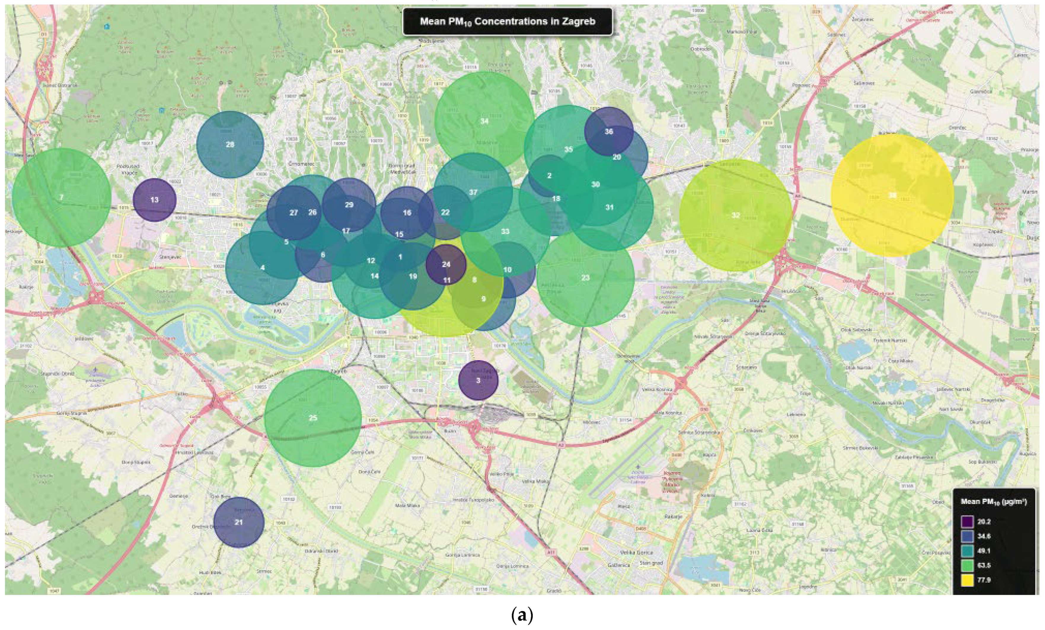
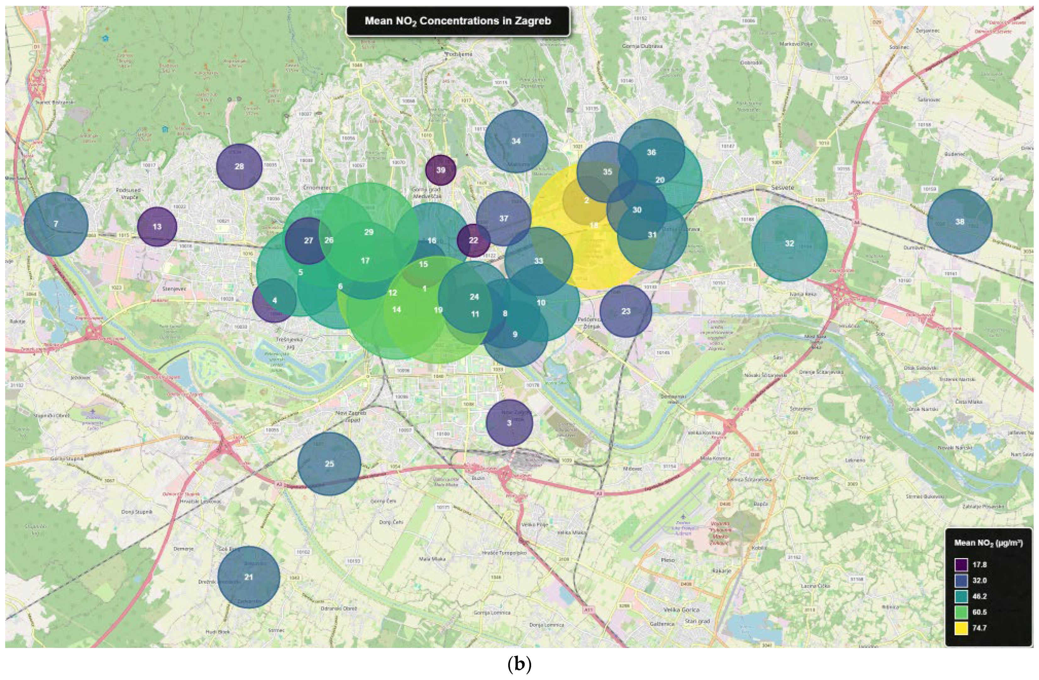
To explore spatial differences in air pollution across Zagreb, average concentrations of NO₂ and PM₁₀ were analyzed for the full observation period (March 2022–May 2024). Figure 2 shows the spatial distribution of mean values per station. The NO₂ map exhibits pronounced spatial variability, with higher concentrations observed in the central and eastern parts of the city, particularly near major traffic corridors and urbanized areas. Sensor locations numbered 18, 19, and 14 (see Table 1) show the highest yearly mean NO₂ concentrations, exceeding 70 µg/m³ and upcoming limit values for the protection of human health (daily up to 50 µg/m³ not more than 18 times per calendar year and annual up to 20 µg/m³), suggesting a significant influence from traffic emissions and localized traffic congestion. On the other hand, in the southern and western parts of the city, at locations 3, 13, and 28, NO₂ levels are notably lower, generally below 30 µg/m³, indicating a reduced anthropogenic influence and the presence of more dispersed residential or green areas.

The distribution of PM₁₀ concentrations is more uniform, with most yearly concentrations falling within the 34–63 µg/m³ range. Nevertheless, a few hotspots, particularly in the eastern urban zones (sites 38 and 32) and one in the center (site 11), show elevated PM10 concentrations. These values, which are mostly above the upcoming limit values for the protection of human health (daily up to 45 µg/m³, not more than 18 times per calendar year, and annual up to 20 µg/m³), may indicate a current combined exposure effect due to vehicular activity, construction, and localized heating sources. Notably, some regions that reported higher NO₂ values do not coincide with the PM₁₀ peaks, indicating that different emission sources and atmospheric processes may be influencing the distribution of each pollutant.

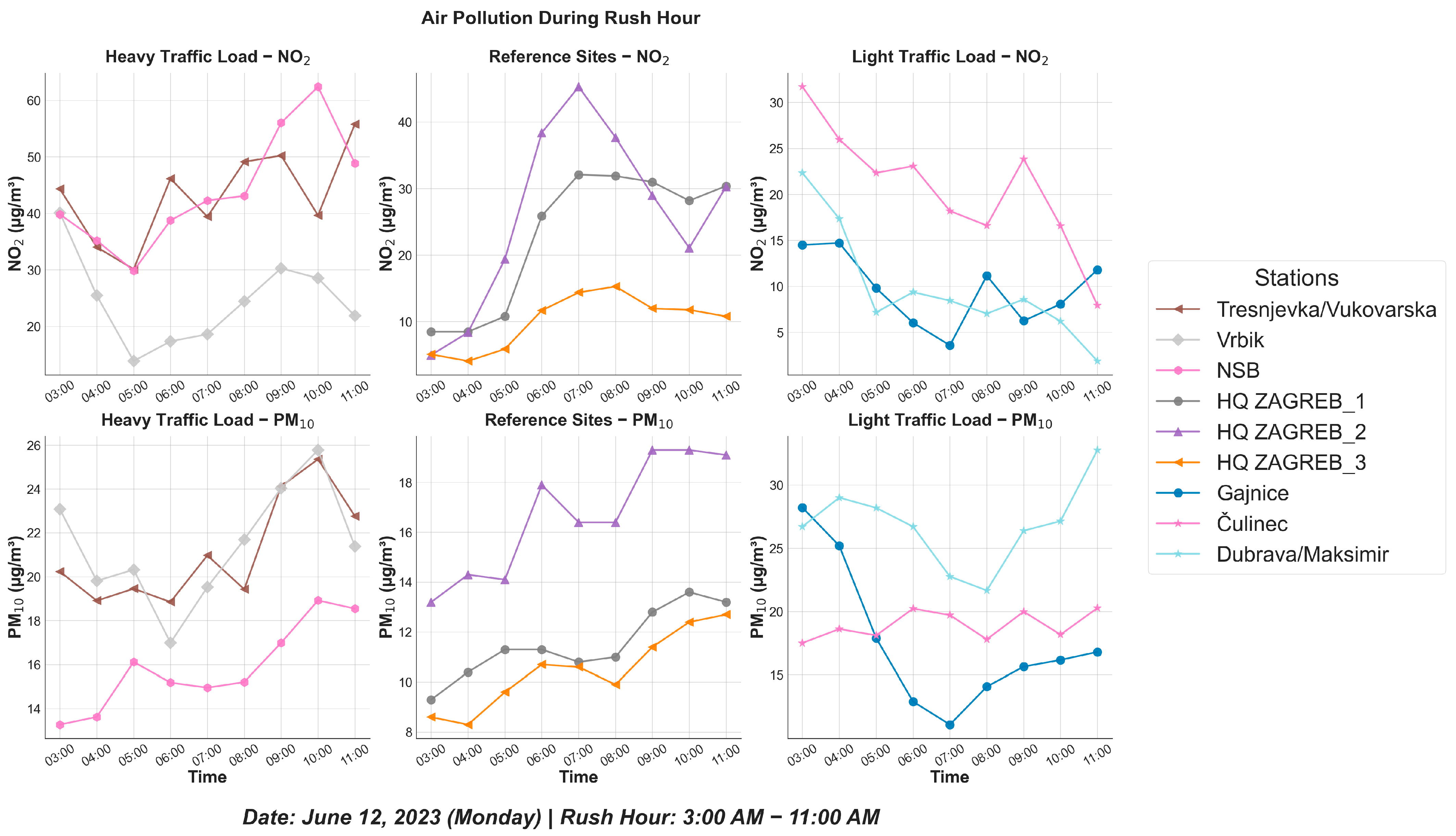
Temporal variations in air pollutant concentrations during the morning rush hour (03:00–11:00) on a randomly selected Monday (12 June 2023) are presented in Figure 3.

Morning hours were chosen because they offer the clearest and most consistent traffic-related emission signal in Zagreb, making them suitable for illustrating how sensors capture rapid, locally driven changes in pollutant concentrations. At the same time, this limited temporal window does not capture the full diurnal or seasonal variability, which is addressed in the long-term analyses presented in other sections. This period was selected as a representative example to highlight traffic-related variations in pollutant concentrations, as it captures the most pronounced contrasts between sites with heavy and low traffic loads. It serves as an illustration of daily variability rather than a complete temporal trend analysis, which is addressed through long-term and aggregated analyses in other sections. As described previously, monitoring locations were grouped into three categories, each comprising three sites. For NO₂, sites with heavy traffic loads exhibited pronounced fluctuations, with peak concentrations observed between 09:00 and 10:00. Maximum levels reached approximately 60 µg/m³ at Trešnjevka/Vukovarska and NSB, while Vrbik showed comparatively lower peaks of around 30 µg/m³. Reference sites displayed a moderate morning increase, with HQ Zagreb-2 reaching ~45 µg/m³, whereas HQ Zagreb-3 remained below 15 µg/m³. In contrast, light traffic load sites maintained consistently lower concentrations, gradually decreasing from early morning peaks (e.g., Čulinec ~32 µg/m³) to 8–12 µg/m³ by 11:00. For PM₁₀, heavy traffic load sites showed a gradual increase in concentrations during the rush hour (26 µg/m³). Reference sites exhibited lower levels, particularly HQ Zagreb-2, which approached 19 µg/m³. Light traffic load sites also have recorded low concentrations, remaining below 20 µg/m³ with only minor fluctuations. Only the Dubrava/Maksimir site showed unusually high PM₁₀ concentrations, which cannot be attributed to traffic. Overall, the results demonstrate the substantial influence of traffic intensity on pollutant concentrations. Heavy traffic load areas were characterized by sharp NO₂ peaks during the morning rush hour, while PM₁₀ concentrations showed less distinct increases but remained elevated at both heavy traffic load and reference sites compared to light traffic load locations. This analysis revealed that sensor data can capture local variations and thereby be used for local health impact analysis of pollution events and air quality assessment in compliance with limit values of PM₁₀ and NO₂ among others for the protection of human health by Directive (EU) 2024/2881 of the European Parliament and of the Council of 23 October 2024 on ambient air quality and cleaner air for Europe [20].

Principle component analysis (PCA) was applied to standardized weekly average concentrations of NO₂ and PM₁₀ across all monitoring stations to understand similarities and differences in pollution behaviour among locations. The left subplot in Figure 4 shows the PCA projection of NO₂ data, while the right subplot presents the corresponding results for PM₁₀. Each point represents a station, labelled by its station number and color-coded for clarity. For NO₂ results, the stations are more widely dispersed in the PCA plot, indicating higher variability in NO₂ pollution profiles across different locations in the city. This spatial spread reflects how local factors such as traffic density and urban structures affect pollution levels at specific stations. In contrast, the PCA of PM₁₀ concentrations revealed a tighter clustering of stations, indicating more uniformity across locations, although some sites (e.g., 1, 5, 11, 31, and 37) still exhibited distinct behavior. Reference-grade DHMZ monitors (stations 1, 2, and 3) appear among the outliers due to their higher precision and calibration standards, while station 39 (ASTIPH reference-grade) was excluded from the PM₁₀ analysis due to insufficient data. The first two principal components (PCs) capture most of the variance for both pollutants, enabling clear visual separation between stations with similar versus distinct pollution profiles.

3.1. Comparison to Reference Measurements

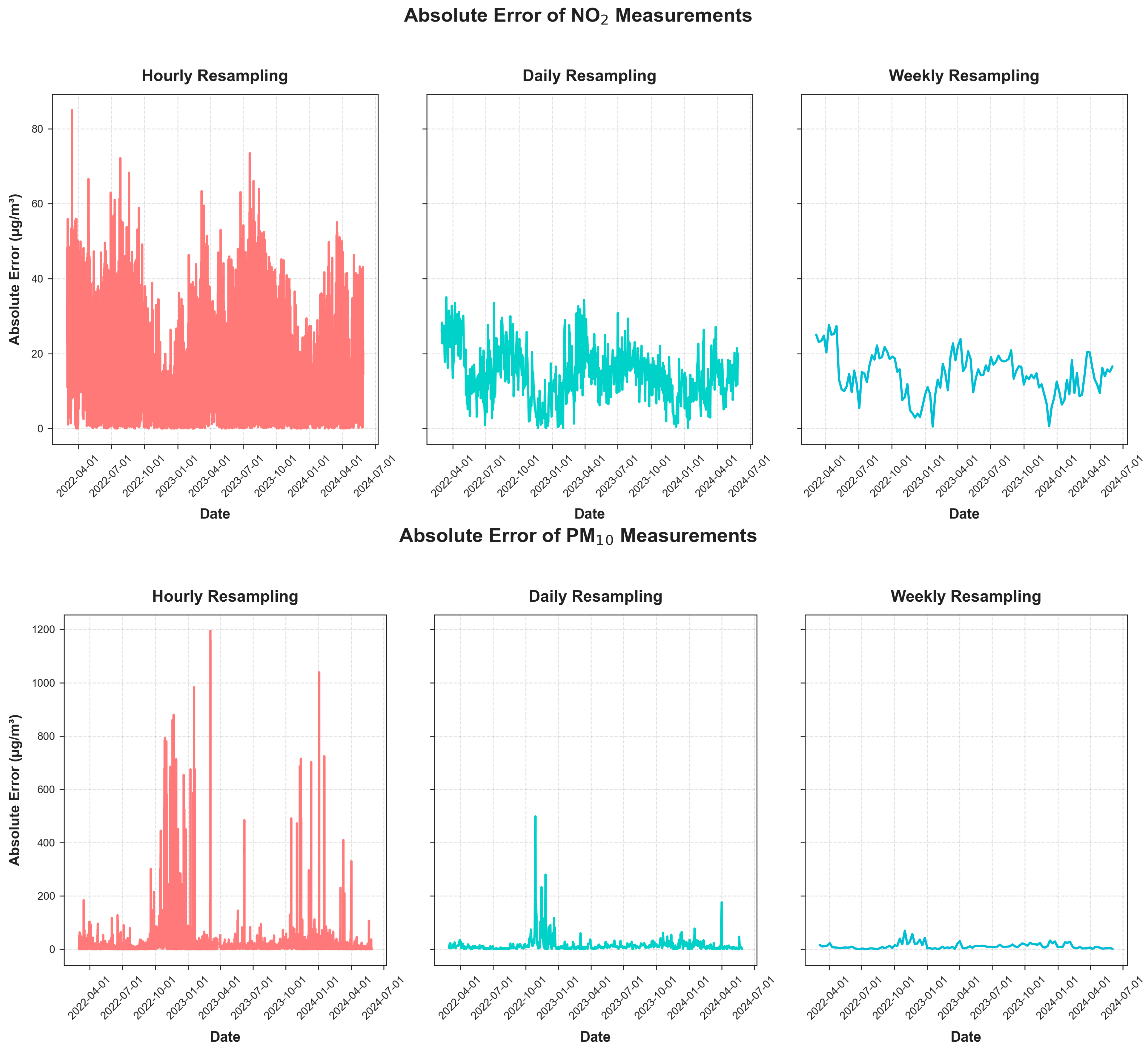
In this section, measurements from the sensors are compared to reference measurements. Figure 5 presents the absolute error of NO₂ and PM₁₀ measurements across three temporal resolutions: hourly, daily, and weekly. To compute the absolute error, measurements from all sensor sites were aggregated by calculating the median, and the same procedure was applied to the reference measurements. The absolute error was then derived from the difference between these aggregated values. These three temporal resolutions were chosen to capture different characteristics: hourly sampling reveals high-frequency fluctuations, daily sampling smooths short-term variations, and weekly sampling highlights long-term error trends. This aggregated error analysis was designed to provide a network-level overview of deviations between the ensemble of sensors and reference stations, explaining temporal and seasonal error patterns rather than quantifying the bias of individual sensors. The upper plot (Figure 5) shows the absolute error of NO₂. Hourly resampling reveals high-frequency fluctuations with peaks exceeding 60 µg/m³, with larger error clusters appearing notably in mid-2022 and 2023. In the daily resampling, while peaks are smoother, the absolute error typically ranges from 10 to 30 µg/m³. Weekly resampling shows relatively stable error values, fluctuating between 10 and 20 µg/m³, with occasional increases. The lower plot in Figure 5 shows the absolute error of PM_10, where hourly resampling exhibits extreme spikes, with errors reaching or exceeding 1200 µg/m³. The distribution is more sporadic than for NO₂, with pronounced outliers, especially in late 2022 and early 2023. Daily resampling reveals clearer temporal patterns, with bursts of error visible around late 2022 and early 2024. Despite smoothing, occasional spikes up to 400 µg/m³ for PM₁₀ persist. Weekly resampling drastically reduces variability, with general error levels below 40 µg/m³, indicating that most extreme fluctuations are short-lived. The analysis shows that as the temporal resolution changes from hourly to weekly, extreme error values are significantly smoothed. This suggests that while high errors do occur, they are typically brief in duration, and daily or weekly averaging provides a more accurate estimation of long-term sensor bias. Given that air quality data are reported as daily values, this suggests sufficient quality for reporting even before software calibration. Moreover, PM₁₀ shows larger and more extreme errors compared to NO₂, especially in the hourly and daily views. This suggests that PM₁₀ predictions from sensors are more sensitive to episodic or extreme pollution events than those of NO₂. Both pollutants exhibit seasonal or periodic errors. For instance, NO₂ errors tend to decrease during late summer and rise again in winter, potentially due to changes in atmospheric dispersion or emission patterns (e.g., increased heating-related emissions in colder months). There is also a visible downward trend in error variability over time, particularly for PM₁₀ during late 2023 and early 2024. This may indicate improvements in the modeling approach or enhanced calibration of the sensor data.

3.2. Sensitivity Assessment

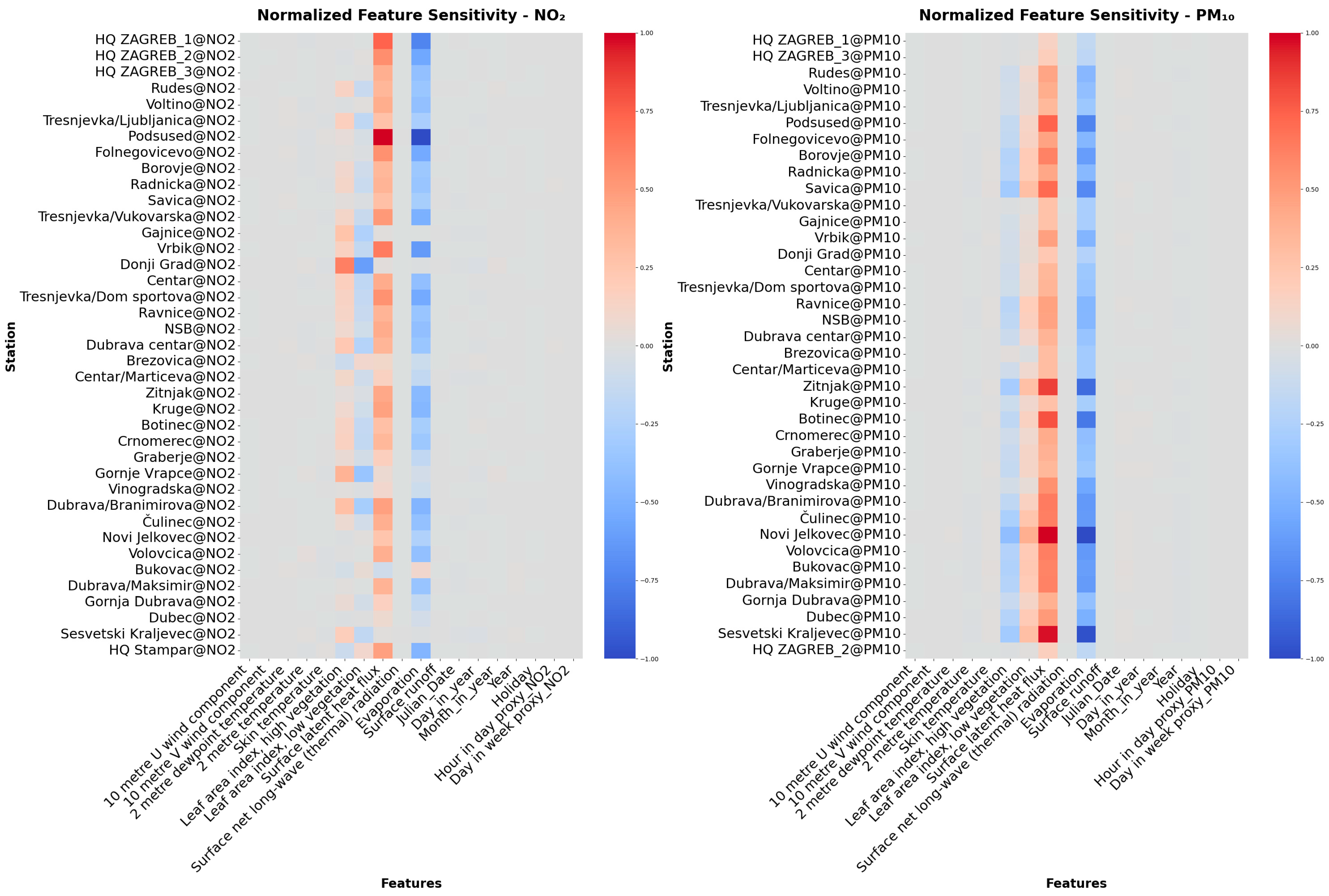
Normalized feature sensitivities for NO₂ (left panel) and PM₁₀ (right panel) concentrations across all monitoring stations are presented in Figure 6. Each row represents a station, while each column corresponds to a feature used in the linear regression model. Feature coefficients were normalized by dividing each value by the maximum absolute coefficient for that station, resulting in values scaled between −1 and 1. This approach emphasizes the relative importance of each feature within a station rather than across stations. For NO₂, most features show values close to zero, indicating weak or diffuse linear relationships with the predictors. Only a few stations display noticeable sensitivity to surface energy balance variables (e.g., surface latent heat flux and evapotranspiration), while temporal features such as Hour in the day or Day in the week contribute very little. This suggests that for NO₂, which is largely traffic-related, the linear model struggles to capture variability using the selected meteorological and temporal predictors. For PM₁₀, sensitivities also remain mostly low across stations. Occasional increases in sensitivity appear for certain stations and meteorological variables, but no consistent feature dominates. Although temporal features have previously been shown to play an important role in PM₁₀ variability [45,46], their contribution here is minimal. Equally important, the overall muted and station-specific sensitivity patterns for both pollutants suggest that neither NO₂ nor PM₁₀ is strongly explained by the selected features within a linear framework. This highlights the need for pollutant-specific calibration strategies and potentially more complex, non-linear model-ling approaches when applying sensor networks for urban air quality monitoring.

3.3. Machine Learning Based Improvement of Data Quality Using Local Stations

ML algorithm XGBoost was used to improve the accuracy of sensor measurements. During the training phase, a Bayesian optimizer was employed to fine-tune the model. The final calibration model utilized the following hyperparameters: n_estimators = 200, indicating that the model was built using 200 decision trees sequentially; and max_depth = 6, which limited the depth of each decision tree, allowing the model to capture moderately complex patterns while reducing the risk of overfitting. A learning rate of 0.1 provided the best balance between learning speed and generalization ability. Subsample of 0.8 implies that 80% of the training data was randomly sampled for each tree, which helped prevent overfitting by introducing variability. For each of the reference stations (1, 2, and 3), two nearby sensor stations were selected. The selection was based on both geographic proximity and similar surrounding environments:

(1)

HQ Zagreb 1 is located on a busy city street with more than six traffic lanes. Therefore, two sensor sites Trešnjevka/Vukovarska and NSB were selected, as both are also located near streets with comparable traffic volume

(2)

HQ Zagreb 2 is situated in the eastern part of the city, which is still relatively busy but less central than HQ Zagreb 1. The chosen sensor sites Dubrava Centar and Ravnice share similar characteristics in terms of the number of surrounding roads and public transport stops

(3)

HQ Zagreb 3 is in the southeastern suburban part of the city, an area with fewer office buildings and lower traffic density. Therefore, Borovje and Folnegovićevo were selected as they share comparable suburban characteristics

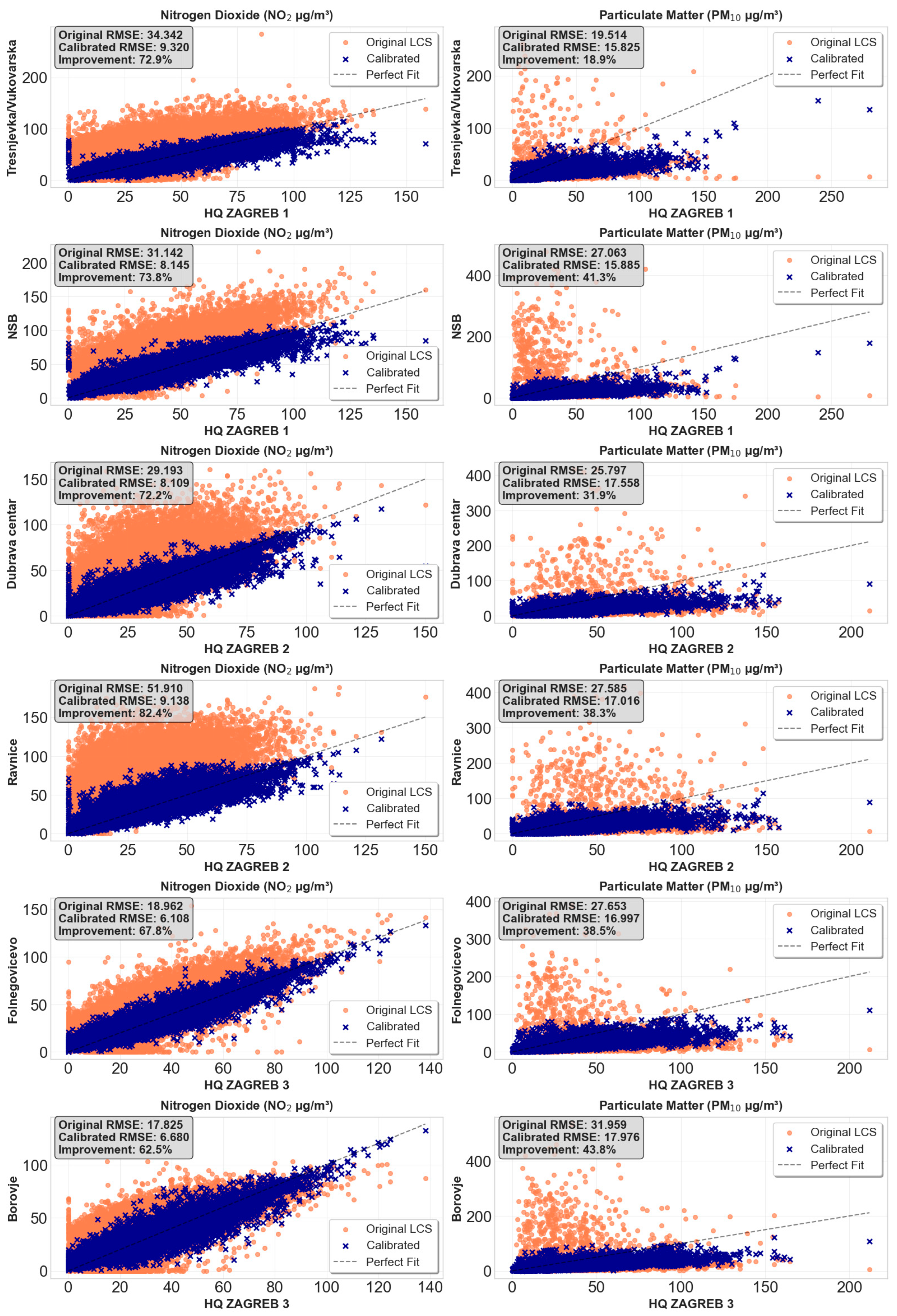
Figure 7 shows the results of the calibration model applied to hourly data. The pre-calibration data are represented as orange dots, while the calibrated values obtained after applying the model are shown in blue. The left column presents results for NO₂, and the right column shows PM₁₀. Each subplot includes the RMSE for the original and calibrated data, along with the calculated percentage improvement. Across all the sensor sites, at higher pollutant concentrations, the original (pre-calibration) data diverges substantially from the reference measurements. The apparent divergence between the sensor and reference data measurements before calibration primarily reflects differences in hyperlocal context. The indicative air quality stations were installed on lighting poles in close proximity to emission sources, up to 4 m above ground and directly facing the street. In contrast, reference-grade stations are generally positioned more than 10 m away from major roads and in semi-open environments to ensure regulatory representativeness. As a result, the indicative sensors often record higher short-term peaks and stronger spatial gradients. These hyperlocal variations naturally lead to discrepancies when comparing sensor data with reference stations, especially without spatial normalization. After calibration, the data points align much more closely with the reference values, indicating a significant improvement in accuracy. The calibration process led to a substantial reduction in RMSE across all sites and for both pollutants. The improvements ranged from 18% to 82%, revealing the effectiveness of the applied correction methodology. The most significant improvement occurred at Ravnice for NO₂, where the RMSE dropped from 51.91 to 9.14 µg/m³², representing an 82% improvement. For PM₁₀, although the initial error levels were generally higher than for NO₂, the calibration still resulted in consistent performance gains, with improvements exceeding 40% in most cases. To better understand the performance of the calibration model over time, rolling RMSE was calculated for both NO₂ and PM₁₀ at each location. This site-specific analysis complements the aggregated error assessment by providing a temporally resolved evaluation of calibration performance, capturing sensor drift and model degradation over time. 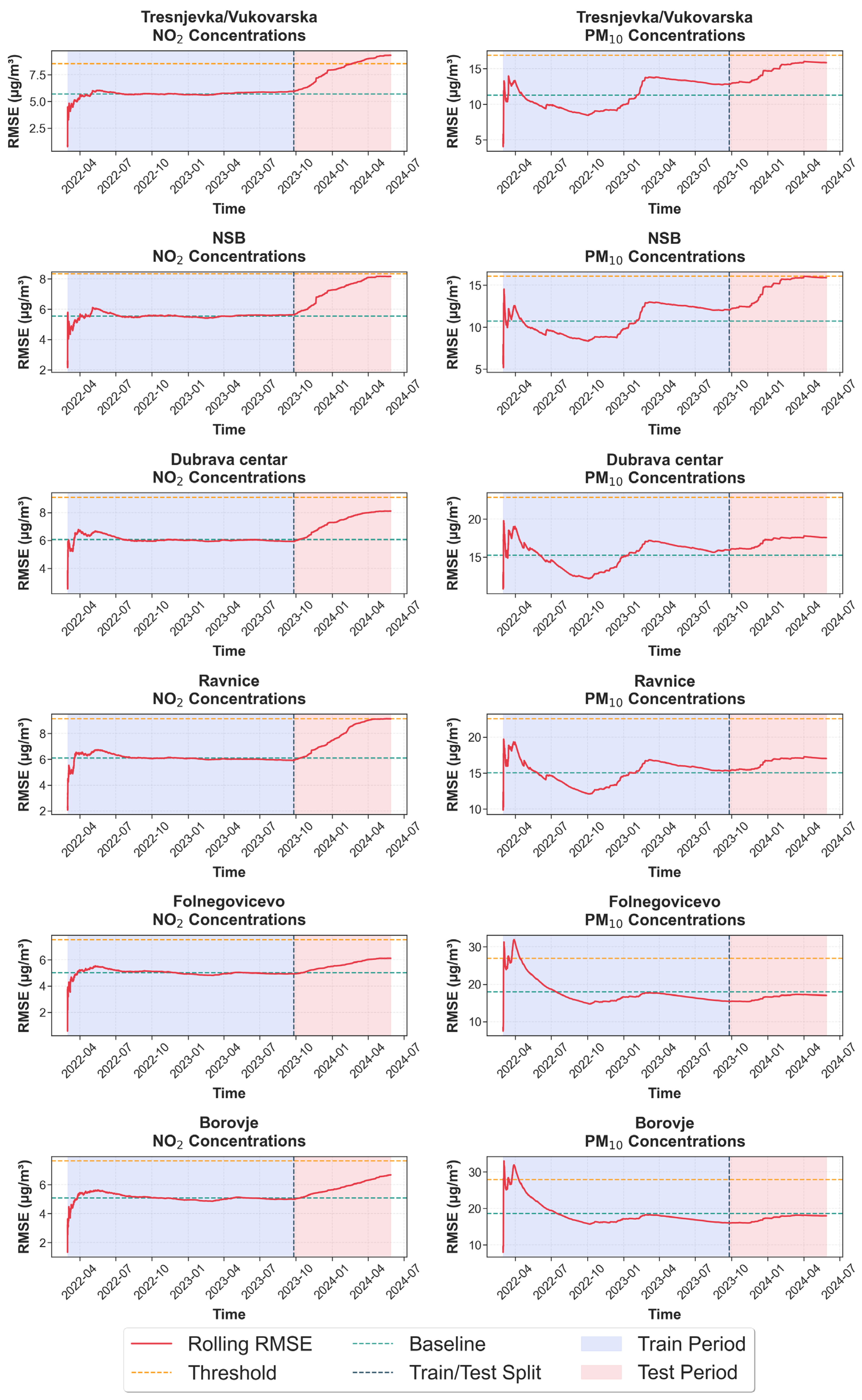Figure 8 shows these results, with NO₂ on the left, and PM₁₀ on the right across all six sensor locations. Each subplot tracks the model’s performance over the entire time span of the dataset. The blue-shaded area represents the training period, while the red-shaded area corresponds to the test period. These two periods are separated by a black vertical dotted line indicating the train/test split. The green dotted line shows the baseline RMSE, calculated during the training phase. The red dashed line represents a threshold that indicates when model recalibration may be necessary. This threshold is defined as a 50% increase over the baseline RMSE. At all locations, model drift is evident during the test period, particularly in 2024, where RMSE increases for both NO₂ and PM₁₀. The increase in RMSE is earlier and more pronounced for PM₁₀, in line with its greater variability and sensitivity. The earliest recalibration is observed at Folnegovićevo station for PM₁₀, just 36 days into the test period, while the latest occurs at Trešnjevka/Vukovarska for NO₂, after 148 days. In some locations, the threshold is not exceeded during the test period, indicating more stable model performance. Notably, Dubrava Centar, Ravnice, and Folnegovićevo stations show rapid error growth, suggesting that these sites may require more frequent retraining or adaptive calibration strategies. The defined thresholds offer a quantitative and interpretable method for identifying when a deployed model’s performance declines to an unacceptable level, supporting effective model maintenance and monitoring practices.

3.4. Strengths and Limitations of the Study

This study presents the first city-wide assessment of next-generation air quality sensors in Zagreb, providing comprehensive spatial and temporal data across 35 sensor locations. A strength of this work lies in the application of ML-based recalibration models (XGBoost), which significantly enhance sensor accuracy, particularly during peak pollution events. Additionally, the introduction of rolling RMSE analysis offers an innovative and practical approach for determining recalibration intervals, contributing to sustainable long-term monitoring practices. The study also integrates extensive meteorological and proxy traffic data, further improving the robustness of sensor calibration.

However, several limitations must be acknowledged. First, full co-location of sensors with reference-grade monitoring stations was not feasible due to infrastructural constraints, leading to reliance on spatiotemporal pairing instead of direct one-to-one calibration. While spatiotemporal pairing provides meaningful correction relationships, it cannot replicate true co-location conditions where micro-environmental differences are eliminated. As a result, some portion of the observed discrepancies particularly short-term peaks reflects hyperlocal emission variability rather than sensor inaccuracy. Moreover, calibration models may partially learn environmental differences rather than purely correcting sensor bias, which should be considered when interpreting the error reductions. Second, the absence of direct traffic data required the use of proxy variables, which may not fully capture real-time traffic dynamics. Although previous studies have shown these proxies to be effective, they cannot fully substitute for real-time traffic data and may underestimate abrupt changes in mobility patterns or special events. Third, while the rolling RMSE method effectively indicates sensor drift, it does not account for the influence of extreme meteorological events or sensor hardware degradation. Lastly, the study focused on PM₁₀ and NO₂ only, while additional pollutants such as PM_2.5, O₃, and CO, though measured, were not included in the calibration analysis.

To address these limitations, future research should aim to increase the number of co-located sensor-reference pairs, integrate real-time traffic and land-use data, and expand calibration efforts to other pollutants and sensor types. Adaptive recalibration frameworks incorporating transfer learning and sensor hardware diagnostics could further improve the scalability and resilience of monitoring networks.

4. Conclusions

This study presents the first city-wide evaluation of air quality sensors in Zagreb, assessing their performance in measuring PM₁₀ and NO₂ concentrations across diverse urban environments prior to software calibration cycles. Unlike previous Croatian studies, this work demonstrates the feasibility of an ML-calibrated, city-wide low-cost sensor network and introduces a replicable recalibration framework based on rolling RMSE. By linking recalibrated data to pollution event detection and health impact relevance, the study provides novel methodological and practical insights for urban air quality management in Europe. The results highlight substantial spatial and temporal variability in these pollutants, which is shaped by traffic, land use, and meteorological conditions. While NO₂ concentrations closely reflected traffic emission patterns, PM₁₀ exhibited a more heterogeneous distribution, influenced by factors such as residential heating, construction activities, and traffic-related factors, including fleet age and road conditions. Sensitivity analysis using linear regression revealed that pollutant concentrations were strongly influenced by temporal and meteorological variables, with NO₂ being more dependent on daily traffic patterns and PM₁₀ more responsive to environmental and surface characteristics. Calibration with XGBoost significantly improved sensor accuracy, reducing RMSE by up to 82%, and should be applied in regular cycles. The models corrected for sensor drift and bias, particularly during peak pollution episodes. Rolling RMSE analysis further indicated that model performance declines over time, especially for PM₁₀, requiring recalibration typically within 1 to 6 months after deployment. While the study demonstrates substantial improvements in sensor performance after ML calibration, these outcomes should be interpreted in the context of several methodological constraints, particularly the reliance on spatiotemporal rather than fully co-located calibration data. Therefore, the results indicate the potential for robust network-wide accuracy rather than establishing strict equivalence to reference-grade measurements. Future work involving expanded co-location campaigns and integration of direct traffic and micro-environmental data will be essential to validate and refine these conclusions. Overall, the findings confirm that an expert-validated sensor system network, when properly calibrated and maintained, serves as a valuable tool for assessing air quality at the city level. This scalable solution for expanding monitoring networks aligns with forthcoming European air quality legislation, enabling more granular data coverage. By combining dense sensor deployments with ML calibration, cities can strengthen evidence-based policy, support targeted public health interventions, and foster citizen engagement in air quality monitoring and management.