Research on the Distribution Characteristics and Health Effects of O₃ in the Fenwei Plain

Abstract

In recent years, coal-combustion-related air pollution has declined markedly, whereas tropospheric ozone (O₃) pollution has emerged as a growing environmental concern. Long-term exposure to O₃ can severely impact human health and ecosystems, constraining socioeconomic development. The Fenwei Plain has complex topographical conditions and a relatively simple industrial structure, and at present, O₃ is one of the main pollutants affecting air quality in this region. Therefore, studying the distribution of O₃ pollution in the Fenwei Plain can provide a reference for developing plans to control O₃ pollution in the area, which is important for safeguarding local public health and economic development. Currently, the number of pollutant monitoring stations in China is limited, spatially discontinuous, and significantly affected by environmental factors, making it difficult to obtain high-precision, large-scale observational data. Satellite-based remote sensing provides broad spatial coverage and is free from topographic constraints, thereby serving as an effective complement to ground-based monitoring networks. This provides important technical support for studying the distribution characteristics of O₃ pollution and its associated health risks. This study focuses on the Fenwei Plain, utilizing machine learning models to estimate continuous O₃ concentrations from 2015 to 2022 and analyze the spatiotemporal distribution of O₃. Based on this, an assessment and analysis of the health risks associated with near-surface O₃ exposure in the study area will be conducted, incorporating the population exposed in the Fenwei Plain and individuals with chronic obstructive pulmonary disease (COPD).

1. Introduction

Nitrogen oxides and volatile organic compounds in the atmosphere produce photochemical smog through photochemical reactions, leading to the formation of ozone [1]. The tropospheric ozone (O₃) is a secondary air pollutant that impacts the health of humans and the ecosystem, and also acts as an important greenhouse gas, being accelerated by and contributing to climate change [2]. Atmospheric ozone has a significant impact on human health, atmospheric chemistry, and climate change [3]. Ozone pollution has become a critical determinant of air quality in China; the Beijing–Tianjin–Hebei region, the Yangtze River Delta, and the Fenwei Plain are particularly notable, with O₃ in these areas exceeding standard levels, accounting for about 70% of the national total from June to September. O₃ is mainly distributed in the stratosphere, with relatively low concentrations near the ground, but it has profound implications for climate change and the ecological environment, causes substantial agricultural production losses [4,5], and affects human health [6], which is associated with increased mortality rates [7,8,9]. O₃ has become one of the main pollutants affecting environmental air quality in some Chinese cities. Long-term exposure to high concentrations of ozone can have serious impacts on human health, agricultural production, and the ecological environment [10,11]. Ozone has a strong oxidative effect on buildings, animals, and plants [12], and different degrees of damage can have varying impacts on the Earth’s ecology and human society [13]. Compared to other gaseous pollutants, ozone has a longer residence time in the troposphere, allowing for long-distance regional transport [14], making O₃ a hot topic in the field of international atmospheric science research. Furthermore, dry deposition is the primary pathway for tropospheric ozone (O₃) removal, with forests playing a critical role. However, environmental stressors such as drought can reduce this removal capacity by limiting stomatal O₃ uptake due to stomata closure [15].

Numerous studies have demonstrated its harmful effects on both ecosystems and human health [6,16]. High concentrations of ground-level ozone can increase urban photochemical smog pollution, irritate the eyes and respiratory tract, impair lung function, and even trigger various diseases. However, there are few studies focusing on the spatiotemporal distribution of ozone and its potential health risks. Most existing analyses of ozone are limited to certain cities, such as Xi’an [17], while research on ozone pollution in the Fenwei Plain is relatively scarce [18,19]. This study analyzes the spatiotemporal distribution characteristics of ozone and its health effects based on observational data on ozone pollutants in the Fenwei Plain. Its aim is to deepen the regional understanding of ozone pollution in the urban agglomeration of the Fenwei Plain, provide a scientific basis for the prevention and control of ozone pollution in the region, and serve as a reference for public health research.

2. Research Area, Data, and Methods

2.1. Overview of the Research Area

This research area employed in this study is the Fenwei Plain, with coordinates ranging from 33.55° to 38.73° N and 106.31°to 114.14° E, as shown in Figure 1. The Fenwei Plain is located in the middle reaches of the Yellow River and is composed of the Fenhe Plain, the Weihe Plain, and surrounding tableland terraces, with an overall orientation from northeast to southwest. The Fenwei Plain belongs to a warm temperate semi-humid climate, characterized by synchronous rainfall and heat, making it the area with the best climatic conditions in the middle reaches of the Yellow River. The Fenhe River basin is elongated from north to south, exhibiting climatic differences between the north and south, while the Weihe River basin shows significant east–west disparities, with precipitation in the western region exceeding that in the eastern region, and heat in the western region being lower than in the eastern region. Additionally, the Fenwei Plain features flat terrain, fertile soil, superior resource conditions, and developed industrial and agricultural sectors, making it one of the seven major production areas in China.

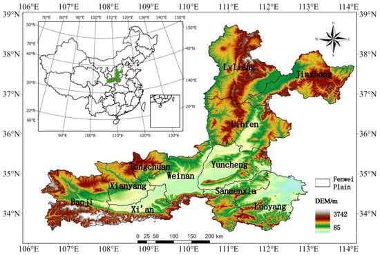
Figure 1. Monitoring station/elevation map of Fenwei Plain.

2.2. Data Sources

This study uses ground monitoring station data, satellite remote sensing data (OMTO3e), meteorological data, ozone precursor data, DEM data, and population data. The ground ozone concentration data was sourced from the National Urban Air Quality Real-time Release Platform of the China Environmental Monitoring Center (https://www.cnemc.cn/) (accessed on 19 August 2023); the satellite remote sensing data was obtained from the Aura Earth Observing System satellite launched by the National Aeronautics and Space Administration (NASA) on 15 July 2004, which is equipped with an Ozone Monitoring Instrument (OMI) [20]; the meteorological data was obtained from the ERA5 hourly reanalysis dataset provided by the European Centre for Medium-Range Weather Forecasts (ECMWF) (https://www.ecmwf.int/en/forecasts/dataset/ecmwf-reanalysis-v5) (accessed on 21 August 2023); the ozone precursor data was derived from the Multi-scale Emission Inventory for China (MEIC) model created by Tsinghua University (http://meicmodel.org.cn/) (accessed on 22 August 2023); the DEM data was sourced from the Geospatial Data Cloud platform (https://www.gscloud.cn/) (accessed on 23 August 2023); and the population density data for the Fenwei Plain region was sourced from the Landscan (https://landscan.ornl.gov/) (accessed on 24 August 2023).

2.3. Research Methods

2.3.1. Random Forest

Random forest (RF), proposed by Breiman et al. [21], is an ensemble learning method based on a large number of decision trees. It randomly selects samples and features based on the ideas of Bagging [22] and random subspace [23]. The random forest algorithm generally shows good agreement between the actual and estimated values. However, when the actual values are extreme, the error between the actual and estimated values can be significant.

2.3.2. eXtreme Gradient Boosting

The XGBoost (eXtreme Gradient Boosting) algorithm is an emerging ensemble learning method based on Gradient Boosting Decision Trees (GBDTs). It was formally introduced by Chen [24] in the 2016 paper “XGBoost: A Scalable Tree Boosting System.” Its core aim is to learn a new function that fits the residuals of the predictions from the previous iteration, thereby training a new tree based on previously generated trees [25]. The advantages of the XGBoost algorithm include support for parallel computation, support for linear base models, random selection of modeling features, built-in cross-validation, regularization to prevent overfitting, and efficient handling of missing data [25].

The calculation formula for the XGBoost model is as follows:

Assuming that K trees have been trained, the final predicted value for the i-th sample is

$$\widehat{{\mathrm{y}}_{\mathrm{i}}}=\sum _{\mathrm{k}=1}^{\mathrm{K}}{\mathrm{f}}_{\mathrm{k}}\left({\mathrm{x}}_{\mathrm{i}}\right),{\mathrm{f}}_{\mathrm{k}}\in \mathcal{F}$$

(1)

where x_i represents the features of the sample, f_k(x_i) is the prediction for the x_i sample using the k-th tree, $\widehat{{\mathrm{y}}_{\mathrm{i}}}$ is the final predicted value, and y_i is the true label of the sample.

The objective function to be constructed needs to include two parts: the training error and regularization. The training error is used to measure the model’s predictive ability on the training data, while regularization is used to control the complexity of the model and prevent overfitting. The calculation formula is as follows:

$$Obj={\sum }_{i=1}^{n}l\left(y_{i,}{\widehat{y}}_i\right)+{\sum }_{k=1}^k\mathsf{\Omega }\left(f_k\right)$$

(2)

where ${\sum }_{i=1}^{n}l\left(y_{i,}{\widehat{y}}_i\right)$ is the loss function, which calculates the loss between the model’s predicted values and the true values, and ${\sum }_{k=1}^k\mathsf{\Omega }\left(f_k\right)$ is the regularization term used to control the complexity of the model and prevent overfitting. In the XGBoost model, the complexity of the regression tree is defined using the following formula:

$$\mathsf{\Omega }\left(f\right)=\gamma T+{\displaystyle \frac{1}{2}}\lambda {‖\omega ‖}^2$$

(3)

where T is the number of leaf nodes on tree f, $\omega$ is a vector composed of the output regression values of all leaf nodes, ${‖\omega ‖}^2$ is the square of the L2 norm (magnitude) of that vector, and $\gamma$ and $\lambda$ are hyperparameters.

The training fit changes in the XGBoost model are illustrated in Figure 2, where the x-axis represents the measured O₃ values from ground stations, and the y-axis represents the estimated values output by the model for the corresponding stations. From the fitting degree plot of the training set (a) and the fitting degree plot of the test set data (b), it can be observed that the points are evenly distributed on both sides of the line y = x. The slope of the fitting curve for the training set model is 0.996, which is close to 1, while the slope of the fitting curve for the test set is 0.794, which is less than 1. The estimated values are slightly higher than the measured values at lower O₃ concentration levels and slightly lower at higher O₃ concentration levels, although the impact is minimal. The coefficient of determination (R²) for the training set is 0.999, with a root mean square error (RMSE) of 0.859 μg/m³ and a bias (BIAS) of −0.001. For the test set, the coefficient of determination (R²) is 0.749, with a root mean square error (RMSE) of 22.379 μg/m³ and a bias (BIAS) of −0.237.

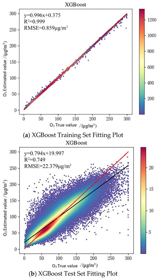
Figure 2. XGBoost ten-fold cross-validation scatter chart. (a) The slope of the fitted curve is 0.996. (b) The slope of the fitted curve is 0.794, both of which are less than 1.

The model testing results obtained from randomly selecting a portion of the test set data in XGBoost are shown in Figure 3. From the figure, it can be observed that the fitting performance is good for most of the data, while the fitting is poor for some instances where the true values are either significantly high or low.

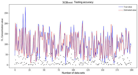
Figure 3. Partial XGBoost test set data testing accuracy.

2.3.3. Support Vector Machine, SVM

Support Vector Machine (SVM) [26] was proposed in 1964 and developed in the 1990s [27] as a type of machine learning method for binary classification of data using supervised learning [28]. SVM uses the hinge loss function to calculate empirical risk and incorporates a regularization term in the optimization process to minimize structural risk, making it a classifier with sparsity and robustness. SVM can perform nonlinear classification through kernel methods and is one of the most common kernel learning methods. The ozone estimates obtained using the support vector machine model often differ significantly from the ground truth measurements, resulting in lower fitting accuracy.

2.3.4. Model Performance Evaluation

The O₃ modeling estimation accuracy of the three machine learning models is shown in Table 1, which shows that the evaluation metrics of the XGBoost model are generally superior to those of RF and SVM. The XGBoost model has the highest degree of agreement between the estimated values for all stations and the ground truth measurements, indicating that the XGBoost model is better at capturing the nonlinear relationships between O₃ and various factors compared to RF and SVM. Table 2 presents a comparison of the fitting accuracy of ozone concentrations in 11 cities of the Fenwei Plain, where the R² and RMSE of the XGBoost model outperform those of RF and SVM. Therefore, the estimation results of the XGBoost model are more accurate.

Table 1. Comparison of modeling accuracy of three machine learning models.

Rating Indicators	Data	RF	XGBoost	SVM
R2	Training Set	0.964	0.999	0.447
	Test Set	0.706	0.749	0.453
RMSE	Training Set	8.753	0.859	30.202
	Test Set	23.341	22.379	30.030
BIAS	Training Set	−0.085	−0.002	−0.013
	Test Set	−0.028	−0.237	−0.423
Slope of the Fitted Curve (k)	Training Set	0.912	0.996	0.640
	Test Set	0.758	0.794	0.645
Intercept of the Fitted Curve (b)	Training Set	8.639	0.375	35.165
	Test Set	23.55	19.997	34.868

Table 2. Comparison of ozone concentration fitting accuracy in 11 cities in the Fenwei Plain.

City	Rating Indicators	RF	XGBoost	SVM
Xi’an	R2	0.766	0.992	0.663
	RMSE	4.927	4.883	30.975
Linfen	R2	0.934	0.992	0.667
	RMSE	2.892	5.078	32.760
Luoyang	R2	0.898	0.991	0.653
	RMSE	4.704	4.917	30.624
Sanmenxia	R2	0.973	0.987	0.635
	RMSE	2.073	5.432	28.695
Xianyang	R2	0.837	0.984	0.628
	RMSE	6.352	6.337	30.975
Tongchuan	R2	0.815	0.982	0.508
	RMSE	4.165	5.810	30.311
Baoji	R2	0.796	0.989	0.590
	RMSE	3.763	4.583	27.389
Weinan	R2	0.639	0.992	0.689
	RMSE	4.778	4.371	27.579
Jinzhong	R2	−1.035	0.991	0.664
	RMSE	4.993	5.076	31.223
Lvliang	R2	−0.700	0.989	0.615
	RMSE	17.588	5.021	29.552

2.3.5. Analysis Methods for Ozone Health Effects

To better assess the exposure levels of ozone in the population, this study calculates the population-weighted exposure concentration of ozone, which incorporates both population distribution and ozone concentration. This approach provides a more accurate reflection of the exposure levels experienced by the population [29,30].

$$c_{wp}={\displaystyle \frac{\sum P_i\times c_i}{\sum P_i}}$$

(4)

In the equation, c_wp represents the population-weighted daily ozone concentration for the entire region, P_i denotes the population density within grid i, and c_i refers to the estimated ozone concentration value within grid i.

In this study, the relative risk (RR) of COPD mortality attributable to ozone exposure is calculated based on the exposure–response relationship between ozone exposure and COPD mortality [31].

$$RR=e^{\left(\beta \times ∆x\right)}$$

(5)

Based on this, the number of COPD deaths attributable to ozone exposure is calculated as follows:

$$PAF={\displaystyle \frac{RR-1}{RR}}$$

(6)

$$\mathsf{\Delta }M=y_0 \mathrm{\ast } PAF \mathrm{\ast } Pop$$

(7)

In the equation, RR represents the relative risk of COPD mortality under ozone concentration exposure; $\beta$ denotes the exposure–response coefficient, indicating that for every increase of 10 μg/m³ in ozone concentration, the risk of COPD mortality increases by approximately 1.4% (95% CI: 0.2%, 5.3%); $\mathsf{\Delta }x$ is the difference between the estimated ozone concentration and the threshold, which is set at 100 μg/m³. If the ozone concentration is below 100 μg/m³, it is considered that ozone exposure has no impact on human health; PAF (Population Attributable Fraction) represents the proportion of COPD cases in the population that can be attributed to ozone exposure; $\mathsf{\Delta }M$ indicates the number of COPD deaths attributable to ozone exposure; y₀ represents the baseline mortality rate for COPD, with data sourced from the national disease monitoring system’s cause of death dataset; and Pop refers to the exposed population, derived from annual statistical yearbooks.

3. Result

3.1. The Spatial Distribution Characteristics of Ozone Pollution in the Fenwei Plain

3.1.1. Annual-Scale Spatial Distribution Characteristics

Using the Kriging interpolation method in ArcGIS Pro 3.1.5, spatial interpolation was performed on the annual average ozone concentration values estimated by the XGBoost model for eleven cities in the Fenwei Plain from 2015 to 2022, resulting in the maps shown in Figure 4 and Figure 5. Figure 4 shows that the annual average ozone concentration during this period ranges between 89.49 μg/m³ and 108.14 μg/m³. Spatially, the ozone concentration generally shows a pattern where higher altitudes correspond to lower ozone concentrations, while lower altitudes correspond to higher ozone concentrations. The areas with high ozone concentrations are concentrated in the cities of Yuncheng, Linfen, Luoyang, Sanmenxia, and Jinzhong, primarily due to the higher population distribution and favorable geographical locations of these areas [32]. Additionally, the central region of the Fenwei Plain is situated in a river valley, where meteorological conditions are stable, making it easier to form ground inversion layers, which can lead to ozone accumulation, thus increasing the ozone concentration in nearby areas. The ozone pollution in Tongchuan City ranks just below that in the five aforementioned cities, primarily due to the rapid development of the secondary industry in the Tongchuan area, resulting in higher emissions of ozone precursors compared to other regions. In contrast, Lvliang City and Baoji City, located at the boundary of the Fenwei Plain, experience relatively lower ozone pollution levels.

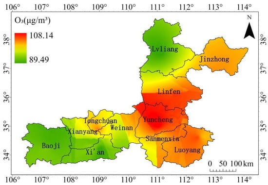
Figure 4. Annual mean spatial distribution of ozone in the Fenwei Plain from 2015 to 2022.

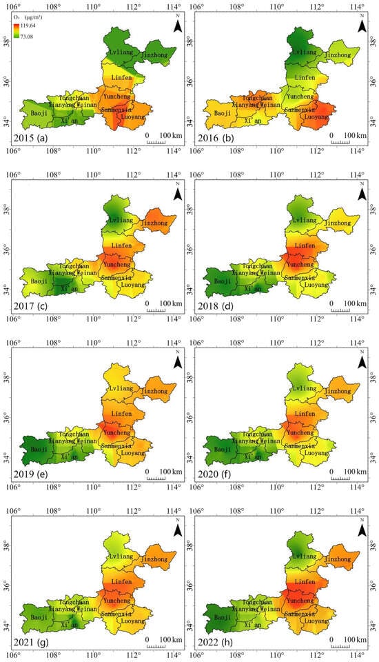
Figure 5. Annual spatial distribution of ozone in the Fenwei Plain from 2015 to 2022. (a–h) Period (2015–2022).

Figure 5 shows the annual average distribution of ozone concentrations in the Fenwei Plain from 2015 to 2022 based on the Kriging interpolation results. It can be observed that the spatial distribution of ozone in the Fenwei Plain generally presents a trend of higher concentrations in the east and lower concentrations in the west, although there are slight variations.

Based on data analysis, we found that in 2017, ozone pollution in the Fenwei Plain was at its most severe. One possible reason for this is that the daily average maximum temperature reached 34.2 °C during June and July of that year, which provided favorable conditions for ozone formation. Starting in 2018, the overall level of ozone pollution in the Fenwei Plain improved, likely due to the government’s designation of the Fenwei Plain as a key area in the “Three-Year Action Plan for Winning the Blue Sky Defense War” issued in 2018. This plan played a significant role in the management and control of various pollutants in the Fenwei Plain region. In 2019, the ozone concentration in the Fenwei Plain decreased compared to previous years, while in 2020, there was a slight increase in ozone concentration.

3.1.2. Seasonal-Scale Spatial Distribution Characteristics

The Fenwei Plain has a warm, temperate, semi-humid climate, so the seasons are divided according to an astronomical perspective: March to May is spring, June to August is summer, September to November is autumn, and December to February is winter. Figure 6 shows the spatial distribution of ozone concentrations in the Fenwei Plain for each season from 2015 to 2022. The results indicate pronounced seasonal variability in ozone concentrations during 2015–2022, following the order of summer > spring > autumn > winter, which is consistent with the findings of Wang Shengjie et al. [33]. In summer, the ozone concentration in the Fenwei Plain ranges from 128.37 μg/m³ to 155.76 μg/m³, while in spring, it ranges from 99.75 μg/m³ to 121.27 μg/m³. In autumn, the ozone concentration ranges from 65.61 μg/m³ to 93 μg/m³, and in winter, it ranges from 45.34 μg/m³ to 74.67 μg/m³, with the maximum difference in ozone concentration reaching 110.42 μg/m³, which is closely related to temperature conditions. From the distribution map, the ozone distribution in spring, summer, and autumn is generally consistent, showing a trend of higher concentrations in the east and lower in the west, as well as higher in the south and lower in the north. Among these, Linfen City and Yuncheng City experience the most severe ozone pollution, which then spreads to the surrounding areas, aligning with the conclusions of Hong Weilin et al. [34].

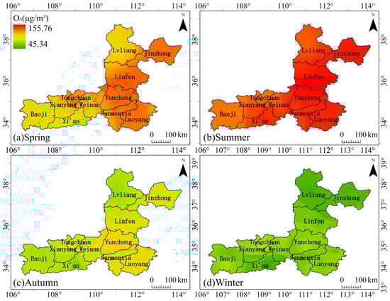
Figure 6. Seasonal spatial distribution of average ozone values in the Fenwei Plain from 2015 to 2022. (a) Spring, (b) summer, (c) autumn, and (d) winter.

3.1.3. Spatial Distribution Characteristics on a Monthly Scale

The analysis of the seasonal average ozone concentrations in the Fenwei Plain demonstrates that, from 2015 to 2022, the formation of ozone pollutants exhibits a significant inter-monthly variation trend. Therefore, it is essential to study inter-monthly spatial variation trends in the Fenwei Plain. Figure 7 illustrates the monthly average spatial distribution of ozone concentrations in the Fenwei Plain from 2015 to 2022.

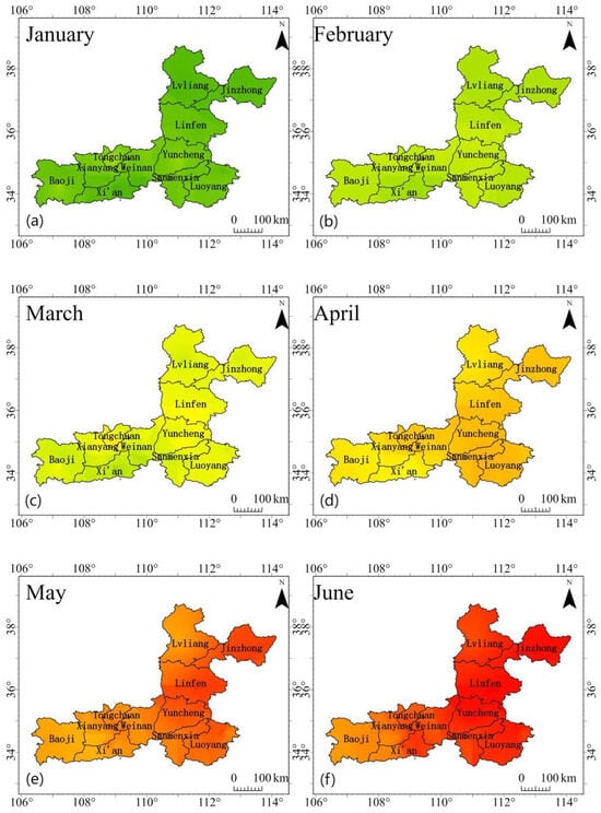
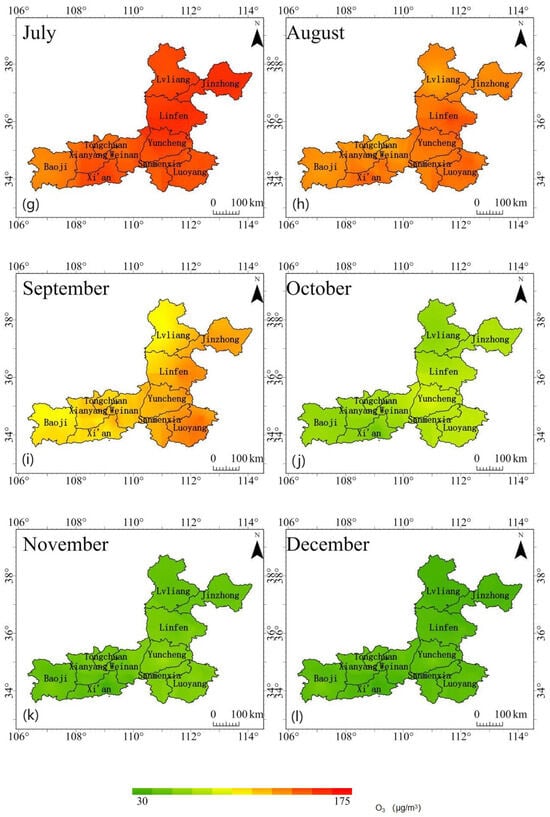
Figure 7. Monthly spatial distribution of ozone in the Fenwei Plain from 2015 to 2022. (a) January, (b) February, (c) March, (d) April, (e) May, (f) June, (g) July, (h) August, (i) September, (j) October, (k) November, and (l) December.

Winter in the Fenwei Plain spans from December to February, during which the ozone concentrations range from 33.1 μg/m³ to 85.09 μg/m³, below 100 μg/m³, indicating that there is slight pollution in the region during winter. The maximum ozone concentration in March is 105.02 μg/m³, exceeding the national first-level limit for ozone. Starting in April, the ozone concentration values gradually increase, with both the maximum and minimum values exceeding 100 μg/m³ from May to August. This indicates that ozone pollution in the Fenwei Plain becomes increasingly severe during this period. After September, the ozone concentration decreases, which aligns with the previous statement that the highest ozone concentrations occur in summer, followed by spring and autumn, with winter having the lowest levels. From a spatial perspective, the distribution of ozone concentrations from October to the following February is relatively uniform. However, from March to September, it is evident that the areas with high levels of ozone are located in the eastern part of the Fenwei Plain. Ozone concentrations are lower in high-altitude areas and higher in low-altitude areas, with urban areas exhibiting higher concentrations than rural areas. In addition, ozone pollution primarily occurs in the spring and summer seasons.

3.1.4. Spatial Autocorrelation Analysis of Ozone

Using ArcGIS Pro 3.1.5, a spatial autocorrelation analysis of the annual average ozone concentrations in the Fenwei Plain from 2015 to 2022 was conducted. The resulting global Moran’s I index, z-scores, and p-values are shown in Table 3. The p-values are all less than 0.01, indicating that the likelihood of this clustering pattern occurring randomly is less than 1%, meaning the confidence interval for the data is over 99%, as confirmed by significance testing.

Table 3. Global Moran’s I index and associated values for annual average ozone concentrations in Fenwei Plain from 2015 to 2022.

Year	Moran’s Index	Z-Scores	p-Values	Variance
2015	0.340641	4.000576	0.000063	0.007909
2016	0.690722	8.013367	0.000000	0.007759
2017	0.702377	8.025032	0.000000	0.007994
2018	0.823737	9.376009	0.000000	0.008005
2019	0.712863	8.107105	0.000000	0.008064
2020	0.862190	9.819896	0.000000	0.007982
2021	0.900472	10.214960	0.000000	0.008035
2022	0.574064	6.560314	0.000000	0.008067
2015–2022	0.809029	9.188001	0.000000	0.008046

Figure 8 shows the LISA clustering maps for the annual and seasonal average ozone concentrations in the Fenwei Plain from 2015 to 2022, illustrating the spatial aggregation characteristics of annual average ozone concentrations over the years. In 2015, Luoyang City exhibited high–high clustering, while Baoji City and Tongchuan City showed high–low clustering, indicating that the ozone concentrations in Luoyang City and its surrounding areas were relatively high, possibly due to spatial diffusion effects. In contrast, although the ozone concentrations in Baoji City and Tongchuan City were high, their surrounding areas had lower ozone concentrations. In 2016, the Fenwei Plain demonstrated spatial aggregation effects, but these were not significant in terms of local spatial autocorrelation. In 2017, Lvliang City displayed low–high clustering, while Baoji City and Tongchuan City continued to show high–low clustering, and Xi’an City exhibited low–low clustering. This indicates that the ozone concentration in Lvliang City was low, with higher concentrations in the surrounding areas, while the opposite was true for Baoji City and Tongchuan City. In 2018, Jinzhong City and its surrounding areas exhibited high–low clustering. In 2019, Tongchuan City, Xianyang City, and Xi’an City showed low–low clustering, indicating that the ozone concentrations in these three cities and their surrounding areas were low, while Luoyang City exhibited high–high clustering, indicating that both Luoyang City and its surrounding areas had high ozone concentrations. In 2020, Tongchuan City and Xi’an City displayed low–low clustering, suggesting that the ozone concentrations in both cities were low, while Jinzhong City showed high–low clustering, indicating that its ozone concentration was higher compared to its surrounding areas. In 2021, Baoji City, Xianyang City, Tongchuan City, and Xi’an City all exhibited low–low clustering, indicating that the ozone concentrations in the western region of the Fenwei Plain were low. In 2022, Jinzhong City and Xi’an City showed high–low clustering, while Yuncheng City exhibited high–high clustering, indicating that the ozone concentrations in Jinzhong City and Xi’an City were high, with lower concentrations in the surrounding areas, whereas Yuncheng City and its surrounding areas had high ozone concentrations.

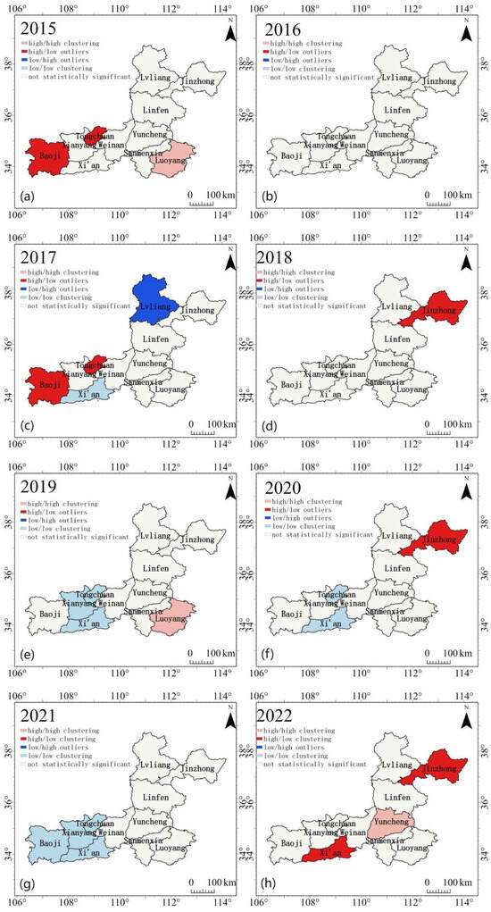
Figure 8. Spatial clustering characteristics of annual average ozone concentration in the Fenwei Plain from 2015 to 2022. (a–h) Period (2015–2022).

3.2. Temporal Distribution Characteristics of Ozone Pollution in the Fenwei Plain

3.2.1. Annual-Scale Temporal Variation

Figure 9 shows an annual average distribution box plot of ozone concentration in the Fenwei Plain from 2015 to 2022, indicating that the overall change in ozone concentration during this period is relatively small, remaining at a high level. Specifically, from 2015 to 2017, the concentration showed a stable upward trend, peaking in 2017. From 2018 to 2020, there was a downward trend, after which the ozone concentration values rose again.

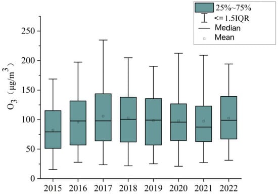
Figure 9. Box plot of annual distribution of ozone concentrations in the Fenwei Plain from 2015 to 2022.

Figure 10, which illustrates the annual classification of the proportions of daily variations in ozone concentration in the Fenwei Plain from 2015 to 2022, shows that ozone pollution in the Fenwei Plain was low in 2015 and 2016. During these years, more than half of the days had ozone concentrations that did not exceed the first-level standard limit, and over 35% of the days did not exceed the second-level standard limit, with days of severe pollution accounting for less than 5%. However, in 2017, the number of days with ozone concentrations exceeding 100 μg/m³ reached half, and more than 3% of the days had ozone concentrations exceeding 200 μg/m³. Starting in 2018, a few years after the government implemented a series of policies to control ozone pollution, ozone levels in the Fenwei Plain began to show slight improvements, with the proportion of “good” days reaching over 50%. Nevertheless, in 2020 and 2021, there were still instances of ozone concentrations exceeding 200 μg/m³. In 2022, the number of days with ozone concentrations below 100 μg/m³ decreased to 51%, indicating a considerable worsening of ozone pollution since 2021.

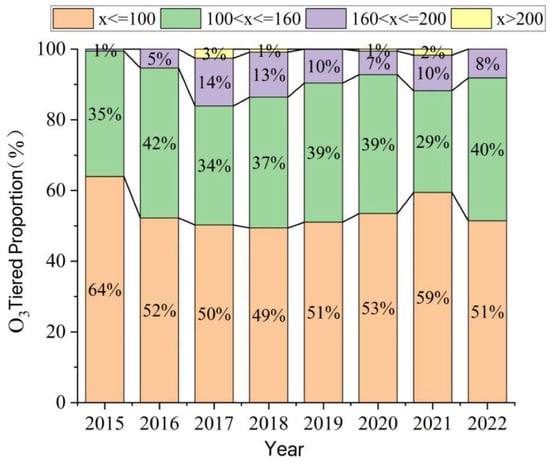
Figure 10. Annual classification of proportions of daily variation in ozone concentration in the Fenwei Plain from 2015 to 2022.

3.2.2. Seasonal-Scale Temporal Variation

Figure 11 illustrates the seasonal variation in ozone concentration in the Fenwei Plain from 2015 to 2022. It shows that the levels of ozone concentration exhibit significant seasonal variation, with each year exhibiting decreasing ozone concentrations in the order of summer > spring > autumn > winter, and a trend of first increasing, then decreasing, and then increasing again.

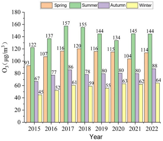
Figure 11. Seasonal average ozone concentration in the Fenwei Plain from 2015 to 2022.

In the process of ozone formation through photochemical reactions, temperature influences various factors such as reaction rate, the release of reactants, and meteorological conditions. Therefore, temperature is closely related to ozone production; low temperatures have a minimal impact on ozone concentration, while increasing temperatures gradually increase ozone levels. Thus, the occurrence of the highest ozone concentration in summer is attributed to strong solar radiation and high temperatures, which promote the occurrence of photochemical reactions. In contrast, spring, autumn, and winter have lower temperatures and weaker sunlight intensity, which are unfavorable for photochemical reactions, resulting in a reduced rate of ozone generation and lower concentration of ozone during these periods. Additionally, in winter, human activities (such as coal heating) produce large amounts of reducing substances like sulfur dioxide, which may affect the redox balance of other substances in the atmosphere, thereby reducing ozone concentration.

3.2.3. Monthly Scale Temporal Variation

The heatmap of monthly average ozone concentrations in the Fenwei Plain (Figure 12) indicates that from 2015 to 2022, the overall trend of ozone concentration in the Fenwei Plain has been increasing. This is primarily characterized by a gradual increase in ozone concentration from January to June, reaching a peak in June, followed by a gradual decline, with the lowest value occurring in December. This finding is consistent with the research results of Qin Zhuofan [35], further confirming the reliability of the XGBoost model for retrieving ozone concentrations. This variation trend is primarily attributed to the combined effects of ultraviolet radiation intensity and favorable meteorological conditions. Firstly, the high temperatures in summer (including June and July) promote ozone generation and, along with excellent sunlight conditions, low wind speeds, and minimal cloud cover, contribute to strong atmospheric stability. These weather conditions increase the photodissociation reactions of oxygen, facilitating photochemical reactions, while also hindering the dispersion of atmospheric pollutants. As a result, the ozone generation rate accelerates during the high-temperature periods of June and July, leading to ozone accumulation near the surface and further increasing its concentration. Secondly, emissions of nitrogen oxides and volatile organic compounds in the atmosphere are higher in summer, and under high temperatures and intense ultraviolet radiation, ozone is generated through photochemical reactions, resulting in peak ozone production during this period.

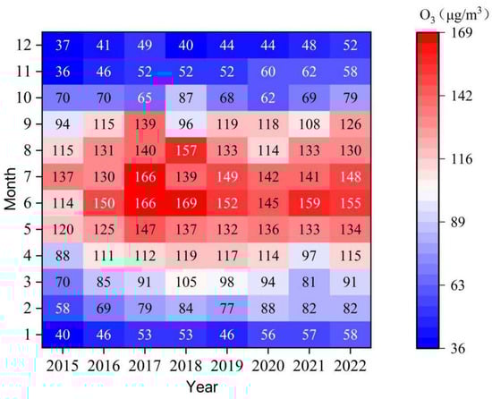
Figure 12. Monthly variations in ozone concentration in the Fenwei Plain from 2015 to 2022.

Figure 13 shows the monthly distribution of ozone concentrations in the Fenwei Plain from 2015 to 2022, demonstrating that the distribution pattern of ozone concentrations for each month of the year presents a “V” shape. This indicates that there is once again severe ozone pollution in the Fenwei Plain. Therefore, the management of ozone pollution in the Fenwei Plain is urgent and cannot be delayed.

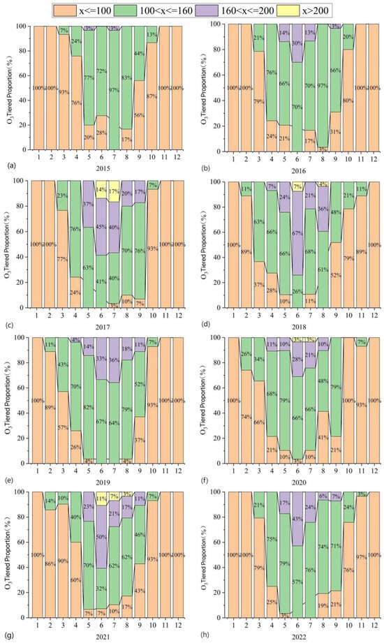
Figure 13. Classification of monthly changes in ozone concentration in the Fenwei Plain. (a–h) Period (2015–2022).

3.3. Health Effect Analysis of Ozone in the Fenwei Plain

To further investigate the impact of ozone pollution on public health, this study analyzes ozone exposure’s burden of mortality due to Chronic Obstructive Pulmonary Disease (COPD), using ozone concentration data simulated by the XGBoost model. The evaluation metrics include ozone population exposure risk, relative risk of COPD, and the number of deaths attributable to ozone. This approach comprehensively considers factors such as ozone concentration, population demographics, and baseline mortality rates for COPD, thereby providing deeper insights into the effects of ozone exposure on public health.

To better assess the exposure levels of ozone in the population, this study calculates the population-weighted exposure concentration of ozone, which incorporates both population distribution and ozone concentration. This approach provides a more accurate reflection of the exposure levels experienced by the population [29,30].

$$c_{wp}={\displaystyle \frac{\sum P_i\times c_i}{\sum P_i}}$$

(8)

In the equation, c_wp represents the population-weighted daily ozone concentration for the entire region, P_i denotes the population density within grid i, and c_i refers to the estimated ozone concentration value within grid i.

In this study, the relative risk (RR) of COPD mortality attributable to ozone exposure is calculated based on the exposure–response relationship between ozone exposure and COPD mortality [31].

$$RR=e^{\left(\beta \times ∆x\right)}$$

(9)

Based on this, the number of COPD deaths attributable to ozone exposure is calculated as follows:

$$PAF={\displaystyle \frac{RR-1}{RR}}$$

(10)

$$\mathsf{\Delta }M=y_0 \mathrm{\ast } PAF \mathrm{\ast } Pop$$

(11)

In the equation, RR represents the relative risk of COPD mortality under ozone concentration exposure; $\beta$ denotes the exposure–response coefficient, indicating that for every increase of 10 μg/m³ in ozone concentration, the risk of COPD mortality increases by approximately 1.4% (95% CI: 0.2%, 5.3%); $\mathsf{\Delta }x$ is the difference between the estimated ozone concentration and the threshold, which is set at 100 μg/m³. If the ozone concentration is below 100 μg/m³, it is considered that ozone exposure has no impact on human health; PAF (Population Attributable Fraction) represents the proportion of COPD cases in the population that can be attributed to ozone exposure; $\mathsf{\Delta }M$ indicates the number of COPD deaths attributable to ozone exposure; y₀ represents the baseline mortality rate for COPD, with data sourced from the national disease monitoring system’s cause of death dataset; and Pop refers to the exposed population, derived from annual statistical yearbooks.

3.3.1. Risk Analysis of Population’s Exposure to Ozone

Figure 14 presents the population-weighted ozone concentrations in the Fenwei Plain region from 2015 to 2022. This is generally consistent with the trend of changes in ozone concentrations in the Fenwei Plain. Overall, the population-weighted annual average ozone concentrations in the Fenwei Plain for the years 2015, 2016, and 2022 were higher than the arithmetic annual average ozone concentrations. In contrast, from 2017 to 2021, the population-weighted annual average ozone concentrations were lower than the arithmetic annual average concentrations. This indicates a clear spatial correlation between ozone concentration and population density in the Fenwei Plain, except for a few years.

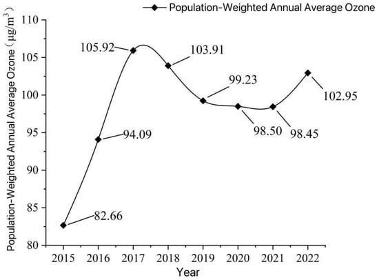
Figure 14. Population-weighted concentrations of ozone in the Fenwei Plain from 2015 to 2022.

3.3.2. Analysis of Relative Risk of Death from Chronic Obstructive Pulmonary Disease (COPD)

Using the ozone concentration data obtained from model simulations for the Fenwei Plain, the relative risk values for ozone exposure and chronic obstructive pulmonary disease (COPD) were calculated using the exposure–response relationship. As shown in Figure 15 and Table 4, areas with higher relative risk values for COPD are generally distributed in the central and eastern regions of the Fenwei Plain, while the northern and western regions, such as Lüliang City, Baoji City, and Xi’an City, have lower relative risk values.

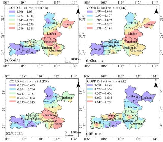
Figure 15. Seasonal spatial distribution of relative risk of COPD mortality in the Fenwei Plain from 2015 to 2022. (a) Spring, (b) summer, (c) autumn, and (d) winter.

Table 4. Annual relative risk of COPD mortality in the Fenwei Plain from 2015 to 2022.

City	Year
	2015	2016	2017	2018	2019	2020	2021	2022
Baoji	0.74	0.98	1.08	0.91	0.83	0.83	0.86	0.94
Jinzhong	0.71	0.85	1.23	1.09	1.10	1.09	1.10	1.11
Linfen	0.78	0.88	1.18	1.30	1.10	1.14	1.17	1.14
Luoyang	0.86	1.13	1.13	1.08	1.09	0.99	1.04	1.08
Lvliang	0.69	0.67	0.94	0.92	1.01	0.90	0.90	0.91
Sanmenxia	0.84	1.03	1.11	1.10	1.01	1.03	1.03	1.07
Tongchuan	0.90	1.11	1.13	1.09	1.00	1.00	0.96	1.02
Weinan	0.76	0.99	1.10	0.97	0.92	0.93	0.97	1.05
Xi’an	0.74	0.90	1.00	0.95	0.87	0.88	0.84	1.00
Xianyang	0.72	0.94	0.98	1.03	0.94	0.92	0.89	0.99
Yuncheng	0.95	0.81	1.26	1.31	1.21	1.19	1.19	1.19

3.3.3. Analysis of the Burden of Deaths Attributable to Chronic Obstructive Pulmonary Disease Due to Ozone Exposure

This study analyzes the burden of deaths from chronic obstructive pulmonary disease (COPD) caused by ozone exposure in the Fenwei Plain and various other cities. Due to the lack of baseline mortality data for COPD in 2022 (Table 5), the analysis of the burden of COPD deaths covers the period from 2015 to 2021. During this period, the analysis results show a fluctuating upward trend, with the most severe burden occurring in 2017, followed by a trend of improvement. However, residents in the Fenwei Plain region remain at significant risk of ozone exposure, and the health hazards posed by ozone continue to exist.

Table 5. Ozone-exposure- and COPD-attributable mortality in the Fenwei Plain from 2015 to 2021.

Year	Exposed Population (Ten Thousand People)	Baseline Mortality Rate (10−5)	Mean Ozone Concentration (μg/m3)	Relative Risk	Population Attributable Fraction (%)	Attributable Deaths (People)
2015	4951.69	60.5	110.343	1.16	13.48	4038
2016	4984.004	59.91	123.745	1.39	28.28	8445
2017	5014.323	56.97	145.7	1.90	47.26	13,501
2018	5056.059	55.6	137.354	1.69	40.72	11,448
2019	5170.397	52.68	135.107	1.64	38.83	10,576
2020	4995.194	45.88	129.726	1.52	34.04	7802
2021	5022.198	46.42	130.749	1.54	34.98	8155

4. Discussion

4.1. Analysis of Ozone Estimation Model’s Accuracy

This study primarily constructs random forest, XGBoost, and support vector machine models to estimate ground-level ozone based on remote sensing data, ground monitoring values, meteorological data, population data, and other geographic covariates. The models are then evaluated using accuracy assessment metrics such as R², RMSE, BIAS, and SD, and the model fitting is further analyzed from a seasonal perspective. Future work could focus on model inversion at the daily scale to improve the precision of the inversion results.

By comparing the experimental results of the random forest and support vector machine algorithms [36], as well as the XGBoost model algorithm. The XGBoost model shows the highest degree of agreement between the estimated values for all sites and the ground-measured values. This suggests that the XGBoost model is better at capturing the nonlinear relationships between O₃ and various factors compared to RF and SVM [26], resulting in the smallest error. The random forest model performs second-best, while the support vector machine model has the lowest fitting accuracy. Some of the data used in the machine learning models only represent a monthly scale, which may affect the accuracy of the inversion results. The efficiency of XGBoost lies in the use of multi-output regressors for multiclass tasks, enhancing generalization compared with other methods [37]. This indicated that the nonlinearity of ozone in relation to several variables, such as precursor levels, meteorology, and spatial variables, became more pronounced at higher ozone concentrations [38]. This stepwise approach enables the capture of complex patterns, including nonlinear relationships, better than single decision trees or linear models [39]. Unlike algorithms that make simpler, isolated predictions, XGBoost considers these interdependencies, which is crucial for accurately estimating fluctuating ozone levels across different regions [40].

4.2. Mechanistic Link Between Ozone Exposure and Chronic Obstructive Pulmonary Disease (COPD)

Chronic obstructive pulmonary disease (COPD) is a chronic condition characterized by a long course, high incidence, and a significant disability rate, affecting patients’ health and productivity [41,42,43]. Previous studies have found positive correlations between long-term O₃ exposure and the incidence, hospital admissions, and mortality rates of COPD [44,45,46]. Ozone exposure can induce the occurrence, development and exacerbation of chronic airway diseases, short-term ozone exposure can induce non-eosinophilic asthma, long-term ozone exposure can induce COPD, and ozone exposure can also induce acute attacks of asthma and acute exacerbation of COPD [47]. This is consistent with epidemiological studies [48,49].

The implementation of the Air Pollution Prevention and Control Action Plan (APPCAP) in China has led to a notable reduction in air pollutants, and yet O₃ concentrations remain persistently high [50,51,52]. The population-weighted annual average concentration of ozone in the Fenwei Plain region shows an increasing trend of fluctuation. For all but a few years, there is a clear spatial matching relationship between ozone concentration and population density in this area. The regions in the Fenwei Plain with a relatively high risk value for COPD-related mortality attributed to ozone exposure are primarily distributed in the central and eastern parts, with the highest relative risk values found in cities such as Yuncheng and Linfen in the central area, which are most affected by ozone concentration levels.

Niu et al. [53] found in a nationwide cohort study on ozone that long-term exposure to ozone increases the risk of mortality from cardiovascular diseases and ischemic heart disease, with a nearly linear relationship between ozone concentration and cardiovascular mortality. The analysis of the burden of COPD mortality attributed to ozone exposure in the Fenwei Plain from 2015 to 2021 shows a fluctuating upward trend, with the most severe burden occurring in 2017, followed by a trend of improvement. However, residents of the Fenwei Plain still face significant risks from ozone exposure. Studies have shown that long-term exposure to ozone can lead to a decline in lung function [54], and the health hazards associated with ozone remain prevalent. Therefore, more reasonable emission reduction policies for ozone should be formulated. And personal protective measures, such as remaining indoors, using air purifiers, wearing face masks, and limiting outdoor physical activities, are essential in reducing individual exposure to O₃ [55].

4.3. Innovation and Limitations

This article analyzes the spatiotemporal distribution characteristics of ozone in the Fenwei Plain from 2015 to 2022 based on machine learning estimation results. It also assesses the health risks of ozone exposure in the region through a population-weighted exposure model and the relative risk of mortality from COPD. However, our study still has the potential for further exploration, and continuous research and in-depth investigation are needed regarding the aforementioned issues.

Due to the lack of long-term population cohort data from China, the exposure–response coefficients and the minimum threshold for ozone exposure used in this study are uncertain. Ground-level O₃ has detrimental effects on human health and crop production; therefore, O₃ concentrations need continuous attention from the scientific community and pollution control authorities [56,57,58]. Additionally, assuming that the baseline mortality rate for COPD is uniform across the study area may lead to over- or underestimation of the evaluation results. Furthermore, future health risk assessments of ozone exposure could consider characteristics such as gender and age, incorporate additional health risk evaluation indicators like disability-adjusted life years (DALY) and years of life lost (YLL) to improve the accuracy of the evaluation results, and study the impact of ozone exposure on socioeconomic benefits.

5. Conclusions

The XGBoost model demonstrates significantly better fitting accuracy than RF and SVM when simulating ozone concentrations in cities of the Fenwei Plain. Furthermore, upon further studying the XGBoost model from a seasonal perspective, it is found that it has the highest estimation accuracy in autumn and winter, followed by spring and summer.

The continuous ozone concentration data obtained using the XGBoost model indicate that the annual average ozone concentration values in the Fenwei Plain from 2015 to 2022 exhibit distinct regional characteristics in the spatial dimension. Areas with high ozone concentrations are primarily located in the central and eastern regions, while low-concentration areas are primarily distributed in the western and northern regions, a pattern that closely aligns with local topographical conditions and industrial structure. Additionally, the distribution of ozone pollution shows strong spatial clustering, with “high–high” clusters found in cities such as Yuncheng and Luoyang, and “low–low” clusters in cities like Tongchuan and Xianyang. From a temporal perspective, the ozone concentration in the Fenwei Plain from 2015 to 2022 shows a trend of increasing fluctuation, remaining at relatively high levels. The ozone concentration also exhibits significant seasonal variation, following a decreasing pattern in the order of summer > spring > autumn > winter. The monthly average ozone concentrations for each year present an inverted “V” shape, with peaks occurring primarily in June and low values occurring in December. The proportion of days with ozone concentrations greater than 100 μg/m³ from 2015 to 2022 in the Fenwei Plain shows an irregular “V” shape.

In the Fenwei Plain, the annual mortality rate of individuals with COPD attributed to ozone exposure is most severe in the central and eastern regions, with Yuncheng and Linfen having the highest relative risk (RR), indicating that these two cities are most affected by ozone exposure, and these relative risk values exhibit significant seasonal characteristics. Furthermore, the COPD mortality burden attributed to ozone exposure in the Fenwei Plain shows a fluctuating upward trend, highlighting the need for targeted management policies to address ozone pollution in the region.

References

- Bloomer, B.J.; Stehr, J.W.; Piety, C.A.; Salawitch, R.J.; Dickerson, R.R. Observed relationships of ozone air pollution with temperature and emissions. Geophys. Res. Lett. 2009, 36, 269–277. [Google Scholar] [CrossRef]
- Fu, T.-M.; Zheng, Y.; Paulot, F.; Mao, J.; Yantosca, R.M. Positive but variable sensitivity of August surface ozone to large-scale warming in the southeast United States. Nat. Clim. Change 2015, 5, 454–458. [Google Scholar] [CrossRef]
- Lefohn, A.S.; Malley, C.S.; Smith, L.; Wells, B.; Hazucha, M.; Simon, H.; Naik, V.; Mills, G.; Schultz, M.G.; Paoletti, E.; et al. Tropospheric ozone assessment report: Global ozone metrics for climate change, human health, and crop/ecosystem research. Elem. Sci. Anthr. 2018, 6, 27. [Google Scholar] [CrossRef] [PubMed]
- Poornima, R.; Dhevagi, P.; Ramya, A.; Agathokleous, E.; Sahasa, R.G.K.; Ramakrishnan, S. Protectants to ameliorate ozone-induced damage in crops—A possible solution for sustainable agriculture. Crop Prot. 2023, 170, 106267. [Google Scholar] [CrossRef]
- Sampedro, J.; Waldhoff, S.T.; Van de Ven, D.-J.; Pardo, G.; Van Dingenen, R.; Arto, I.; del Prado, A.; Sanz, M.J. Future impacts of ozone driven damages on agricultural systems. Atmos. Environ. 2020, 231, 117538. [Google Scholar] [CrossRef]
- Tao, C.; Mettke, P.; Wang, Y.; Li, X.; Hu, L. Exhalation metabolomics: A new force in revealing the impact of ozone pollution on respiratory health. Eco-Environ. Health 2024, 3, 407–411. [Google Scholar] [CrossRef]
- Yan, D.; Jin, Z.; Zhou, Y.; Li, M.; Zhang, Z.; Wang, T.; Zhuang, B.; Li, S.; Xie, M. Anthropogenically and meteorologically modulated summertime ozone trends and their health implications since China’s clean air actions. Environ. Pollut. 2024, 343, 123234. [Google Scholar] [CrossRef]
- Yang, X.; Wang, L.; Ma, P.; He, Y.; Zhao, C.; Zhao, W. Urban and suburban decadal variations in air pollution of Beijing and its meteorological drivers. Environ. Int. 2023, 181, 108301. [Google Scholar] [CrossRef]
- Huang, M.; Tao, S.; Zhu, K.; Feng, H.; Lu, X.; Hang, J.; Wang, X. Applicability of evaluation metrics/schemes for human health burden attributable to regional ozone pollution: A case study in the Guangdong-Hong Kong-Macao Greater Bay Area (GBA), South China. Sci. Total Environ. 2024, 914, 169910. [Google Scholar] [CrossRef]
- Chen, R.; Chen, B.; Kan, H. Health impact assessment of surface ozone pollution in Shanghai. China Environ. Sci. 2010, 30, 603–608. [Google Scholar]
- Jia, L.; Ge, M.; Xu, Y.; Du, L.; Zhuang, G.; Wang, D. Advances in Atmospheric Ozone Chemistry. Prog. Chem. 2006, 18, 1565–1574. [Google Scholar]
- Lee, D.S.; Holland, M.R.; Falla, N. The potential impact of ozone on materials in the U.K. Atmos. Environ. 1996, 30, 1053–1065. [Google Scholar] [CrossRef]
- Liu, F.; Zhu, Y.; Wang, X. Surface ozone pollution and its ecoenvironmental impacts in China. Ecol. Environ. 2008, 4, 1674–1679. [Google Scholar]
- Fiore, A.M.; Dentener, F.J.; Wild, O.; Cuvelier, C.; Schultz, M.G.; Hess, P.; Textor, C.; Schulz, M.; Doherty, R.M.; Horowitz, L.W. Multimodel estimates of intercontinental source-receptor\nrelationships for ozone pollution. J. Geophys. Res. D Atmos. 2009, 114, D04301. [Google Scholar] [CrossRef]
- Juráň, S.; Karl, T.; Ofori-Amanfo, K.K.; Šigut, L.; Zavadilová, I.; Grace, J.; Urban, O. Drought shifts ozone deposition pathways in spruce forest from stomatal to non-stomatal flux. Environ. Pollut. 2025, 372, 126081. [Google Scholar] [CrossRef]
- Day, D.B.; Xiang, J.; Mo, J.; Li, F.; Chung, M.; Gong, J.; Weschler, C.J.; Ohman-Strickland, P.A.; Sundell, J.; Weng, W.; et al. Association of Ozone Exposure with Cardiorespiratory Pathophysiologic Mechanisms in Healthy Adults. JAMA Intern. Med. 2017, 177, 1344–1353. [Google Scholar] [CrossRef] [PubMed]
- Lu, D.; Dong, Z.; Cao, H.; Li, X. Characteristics of ozone pollution and its relationship with the meteorological conditions in Xi’an. J. Shaanxi Meteorol. 2020, 1, 14–19. [Google Scholar]
- Cai, H.; Lu, E.; Chen, X.; Liu, P.; Zhong, M. PM2.5 distribution and its relationship with meteorological elements in Gaoling District. J. Shaanxi Meteorol. 2021, 5, 42–46. [Google Scholar]
- Wang, H.; He, X.; Su, J.; Ma, Y. Analysis of the spatiotemporal distribution of major air pollutants in Guanzhong region. J. Shaanxi Meteorol. 2020, 3, 26–30. [Google Scholar]
- Chen, Y.; Chen, C.; Liu, Z.; Hu, Z.; Wang, X. The methodology function of Cite Space mapping knowledge domains. Stud. Sci. Sci. 2015, 33, 242–253. [Google Scholar]
- Breiman, L. Random Forests. Mach. Learn. 2001, 45, 5–32. [Google Scholar] [CrossRef]
- Breiman, L. Bagging Predictors. Mach. Learn. 1996, 24, 123–140. [Google Scholar] [CrossRef]
- Tin Kam, H. The random subspace method for constructing decision forests. IEEE Trans. Pattern Anal. Mach. Intell. 1998, 20, 832–844. [Google Scholar] [CrossRef]
- Chen, T.; Guestrin, C. XGBoost: A Scalable Tree Boosting System. In Proceedings of the 22nd ACM SIGKDD International Conference on Knowledge Discovery and Data Mining, San Francisco, CA, USA, 13–17 August 2016. [Google Scholar]
- Zhou, Y. Research on AQI Prediction Model ofHefei City Based on Boosting Algorithm. Master’s Thesis, Anhui University of Finance and Economics, Bengbu, China, 2021. [Google Scholar]
- Saunders, C.; Stitson, M.O.; Weston, J.; Holloway, R.; Bottou, L.; Scholkopf, B.; Smola, A. Support Vector Machine. Comput. Ence 2002, 1, 1–28. [Google Scholar]
- Tan, X.; Chen, J.; Cao, J.; Hu, L.; Li, C.; Zhou, H. Application and Comparison of Logistic Regression and Support Vector Machine in Condition Assessment of Cable Aging Condition. High Volt. Appar. 2023, 59, 113–121. [Google Scholar] [CrossRef]
- Vapnik, V.N. Statistical Learning Theory (Adaptive and Learning Systems for Signal Processing, Communications and Control Series); Wiley: Hoboken, NJ, USA, 1998; Volume 10–11, pp. 401–492. [Google Scholar]
- Hu, J.; Ying, Q.; Chen, J.; Mahmud, A.; Zhao, Z.; Chen, S.-H.; Kleeman, M.J. Particulate air quality model predictions using prognostic vs. diagnostic meteorology in central California. Atmos. Environ. 2010, 44, 215–226. [Google Scholar] [CrossRef]
- Liu, T.; Wang, C.; Wang, Y.; Huang, L.; Li, J.; Xie, F.; Zhang, J.; Hu, J. Impacts of model resolution on predictions of air quality and associated health exposure in Nanjing, China. Chemosphere 2020, 249, 126515. [Google Scholar] [CrossRef]
- Zhao, N.; Lu, Y. Estimation of Surface Ozone Concentration and Health Impact Assessment in China. Environ. Sci. 2022, 43, 1235–1245. [Google Scholar] [CrossRef]
- Xia, L.; Wang, J.; Huang, Y.; Wang, R.; Wang, R. Lung cancer risk assessment of the exposure to atmospheric polycyclicaromatic hydrocarbons based on population attributable fraction andincremental lifetime cancer risk models: A case study in Hefei. Environ. Chem. 2024, 43, 856–863. [Google Scholar]
- Wang, S.; Xie, S.; Wang, J.; Huo, X.; Wang, W.; Du, L. Analysis of Air Quality in Fenwei Plain from 2016 to 2019. Environ. Monit. China 2020, 36, 57–65. [Google Scholar] [CrossRef]
- Hong, W.; Miao, Y.; Jia, X.; Sun, F.; Luo, H.; Hong, H.; Wang, M. Spatiotemporal Distribution Characteristics and Population Exposure of Air Pollution in the Fenwei Plain from 2015 to 2020. J. Anhui Norm. Univ. (Nat. Sci.) 2023, 46, 457–465. [Google Scholar] [CrossRef]
- Qin, Z.; Liao, H.; Chen, L.; Zhu, J.; Qian, J. Fenwei Plain Air Quality and the Dominant Meteorological Parameters for Its Daily and Interannual Variations. Chin. J. Atmos. Sci. 2021, 45, 1273–1291. (In Chinese) [Google Scholar]
- Li, H.; Dong, P.; Li, Y. Engine Health Status Assessment Based on SVM. Ship Electron. Eng. 2023, 43, 158–163. [Google Scholar]
- Emami, S.; Martínez-Muñoz, G. Condensed-gradient boosting. Int. J. Mach. Learn. Cybern. 2025, 16, 687–701. [Google Scholar] [CrossRef]
- Vicente, D.J.; Salazar, F.; López-Chacón, S.R.; Soriano, C.; Martin-Vide, J. Evaluation of different machine learning approaches for predicting high concentration episodes of ground-level ozone: A case study in Catalonia, Spain. Atmos. Pollut. Res. 2024, 15, 101999. [Google Scholar] [CrossRef]
- Si, M.; Du, K. Development of a predictive emissions model using a gradient boosting machine learning method. Environ. Technol. Innov. 2020, 20, 101028. [Google Scholar] [CrossRef]
- Imami, A.D.; Yee, J.-J. Neighborhood ozone estimation in Busan, South Korea: A comparative study of proximity-based ensemble clustering and machine-learning models. Atmos. Pollut. Res. 2025, 16, 102601. [Google Scholar] [CrossRef]
- Celli, B.; Fabbri, L.; Criner, G.; Martinez, F.J.; Mannino, D.; Vogelmeier, C.; Montes de Oca, M.; Papi, A.; Sin, D.D.; Han, M.K.; et al. Definition and Nomenclature of Chronic Obstructive Pulmonary Disease: Time for Its Revision. Am. J. Respir. Crit. Care Med. 2022, 206, 1317–1325. [Google Scholar] [CrossRef]
- Liang, Z.; Wang, F.; Chen, Z.; Chen, R. Updated Key Points Interpretation of Global Strategy for the Diagnosis, Management, and Prevention of Chronic Obstructive PulmonaryDisease(2023 Report). Chin. Gen. Pract. 2023, 26, 1287–1298. [Google Scholar]
- Diagnostic Guidelines for Chronic Obstructive Pulmonary Disease (Revised 2021 Edition). Pract. J. Card. Cereb. Pneumal Vasc. Dis. 2021, 29, 134.
- Lim, C.C.; Hayes, R.B.; Ahn, J.; Shao, Y.; Silverman, D.T.; Jones, R.R.; Garcia, C.; Bell, M.L.; Thurston, G.D. Long-Term Exposure to Ozone and Cause-Specific Mortality Risk in the United States. Am. J. Respir. Crit. Care Med. 2019, 200, 1022–1031. [Google Scholar] [CrossRef]
- Press, V.G.; Konetzka, R.T.; White, S.R. Insights about the economic impact of chronic obstructive pulmonary disease readmissions post implementation of the hospital readmission reduction program. Curr. Opin. Pulm. Med. 2018, 24, 138–146. [Google Scholar] [CrossRef]
- Shin, S.; Bai, L.; Burnett, R.T.; Kwong, J.C.; Hystad, P.; van Donkelaar, A.; Lavigne, E.; Weichenthal, S.; Copes, R.; Martin, R.V.; et al. Air Pollution as a Risk Factor for Incident Chronic Obstructive Pulmonary Disease and Asthma. A 15-Year Population-based Cohort Study. Am. J. Respir. Crit. Care Med. 2021, 203, 1138–1148. [Google Scholar] [CrossRef]
- Wen, J.; Li, C.; Li, F. Advances in research on effects and mechanisms of ozone exposure on asthma and chronicobstructive pulmonary disease. J. Environ. Occup. Med. 2023, 40, 965–971. [Google Scholar]
- Jerrett, M.; Burnett, R.T.; Pope, C.A., III; Ito, K.; Thurston, G.; Krewski, D.; Shi, Y.; Calle, E.; Thun, M. Long-term ozone exposure and mortality. N. Engl. J. Med. 2009, 360, 1085–1095. [Google Scholar] [CrossRef] [PubMed]
- Seinfeld, J.H.; Pandis, S.N.; Noone, K. Atmospheric Chemistry and Physics: From Air Pollution to Climate Change. Phys. Today 2008, 51, 88. [Google Scholar] [CrossRef]
- Liang, L.; Cai, Y.; Barratt, B.; Lyu, B.; Chan, Q.; Hansell, A.L.; Xie, W.; Zhang, D.; Kelly, F.J.; Tong, Z. Associations between daily air quality and hospitalisations for acute exacerbation of chronic obstructive pulmonary disease in Beijing, 2013–2017: An ecological analysis. Lancet Planet. Health 2019, 3, e270–e279. [Google Scholar] [CrossRef]
- Huang, J.; Pan, X.; Guo, X.; Li, G. Health impact of China’s Air Pollution Prevention and Control Action Plan: An analysis of national air quality monitoring and mortality data. Lancet Planet. Health 2018, 2, e313–e323. [Google Scholar] [CrossRef]
- Xue, T.; Zhu, T.; Peng, W.; Guan, T.; Zhang, S.; Zheng, Y.; Geng, G.; Zhang, Q. Clean air actions in China, PM2.5 exposure, and household medical expenditures: A quasi-experimental study. PLoS Med. 2021, 18, e1003480. [Google Scholar] [CrossRef]
- Niu, Y.; Zhou, Y.; Chen, R.; Yin, P.; Meng, X.; Wang, W.; Liu, C.; Ji, J.S.; Qiu, Y.; Kan, H.; et al. Long-term exposure to ozone and cardiovascular mortality in China: A nationwide cohort study. Lancet Planet. Health 2022, 6, e496–e503. [Google Scholar] [CrossRef] [PubMed]
- Crouse, D.L.; Peters, P.A.; Hystad, P.; Brook, J.R.; van Donkelaar, A.; Martin, R.V.; Villeneuve, P.J.; Jerrett, M.; Goldberg, M.S.; Pope, C.A., 3rd; et al. Ambient PM2.5, O3, and NO2 Exposures and Associations with Mortality over 16 Years of Follow-Up in the Canadian Census Health and Environment Cohort (CanCHEC). Environ. Health Perspect. 2015, 123, 1180–1186. [Google Scholar] [CrossRef]
- Laumbach, R.J.; Cromar, K.R. Personal Interventions to Reduce Exposure to Outdoor Air Pollution. Annu. Rev. Public Health 2022, 43, 293–309. [Google Scholar] [CrossRef] [PubMed]
- Wan, W.; Manning, W.J.; Wang, X.; Zhang, H.; Sun, X.; Zhang, Q. Ozone and ozone injury on plants in and around Beijing, China. Environ. Pollut. 2014, 191, 215–222. [Google Scholar] [CrossRef] [PubMed]
- Feng, Z.; Hu, E.; Wang, X.; Jiang, L.; Liu, X. Ground-level O3 pollution and its impacts on food crops in China: A review. Environ. Pollut. 2015, 199, 42–48. [Google Scholar] [CrossRef] [PubMed]
- Chuwah, C.; van Noije, T.; van Vuuren, D.P.; Stehfest, E.; Hazeleger, W. Global impacts of surface ozone changes on crop yields and land use. Atmos. Environ. 2015, 106, 11–23. [Google Scholar] [CrossRef]
Disclaimer/Publisher’s Note: The statements, opinions and data contained in all publications are solely those of the individual author(s) and contributor(s) and not of MDPI and/or the editor(s). MDPI and/or the editor(s) disclaim responsibility for any injury to people or property resulting from any ideas, methods, instructions or products referred to in the content. |
© 2025 by the authors. Licensee MDPI, Basel, Switzerland. This article is an open access article distributed under the terms and conditions of the Creative Commons Attribution (CC BY) license (https://creativecommons.org/licenses/by/4.0/).