Advanced Soft Computing Techniques for Monthly Streamflow Prediction in Seasonal Rivers

Abstract

The rising incidence of droughts in specific global regions in recent years, primarily attributed to global warming, has markedly increased the demand for reliable and accurate streamflow estimation. Streamflow estimation is essential for the effective management and utilization of water resources, as well as for the design of hydraulic infrastructure. Furthermore, research on streamflow estimation has gained heightened importance because water is essential not only for the survival of all living organisms but also for determining the quality of life on Earth. In this study, advanced soft computing techniques, including long short-term memory (LSTM), convolutional neural network–recurrent neural network (CNN-RNN), and group method of data handling (GMDH) algorithms, were employed to forecast monthly streamflow time series at two different stations in the Wadi Mina basin. The performance of each technique was evaluated using statistical criteria such as mean square error (MSE), mean bias error (MBE), mean absolute error (MAE), and the correlation coefficient (R). The results of this study demonstrated that the GMDH algorithm produced the most accurate forecasts at the Sidi AEK Djillali station, with metrics of MSE: 0.132, MAE: 0.185, MBE: −0.008, and R: 0.636. Similarly, the CNN-RNN algorithm achieved the best performance at the Kef Mehboula station, with metrics of MSE: 0.298, MAE: 0.335, MBE: −0.018, and R: 0.597.

1. Introduction

Accurate prediction of streamflow is critical for the development and management of water resources in many parts of the world. This includes applications such as flood control, dam design and construction, the implementation of hydraulic structures like bridges, reservoir operation and management, water supply, and hydroelectric power generation. However, due to the basin’s erratic flow distribution, periodic flow patterns, and complex, non-linear interactions between its constituent elements—such as climatic conditions, soil type, and vegetation cover—accurately estimating a catchment’s streamflow remains a significant challenge.

In recent decades, numerous studies have been reported on streamflow modeling via machine learning (ML) approaches. Mehdizadeh and Kozekalani Sales [1] evaluated the efficiency of artificial intelligence (AI) methods for estimating monthly streamflow in Northern Iran over the period from October 1964 to September 2014. These methods included Bayesian networks (BNs), gene expression programming (GEP), autoregressive (AR), and autoregressive moving average (ARMA), as well as simple multiple linear regression (MLR). The study revealed that the BN2-AR model at Ponel station and the BN4-AR model at Toolelat station provided the most accurate streamflow estimations. Al-Juboori [2] applied random tree (RT) and K-nearest neighbor (KNN) algorithms to estimate the streamflow data in Iraq. The results showed that the KNN-RT hybrid model produced promising outputs. Zhu et al. [3] implemented probabilistic long short-term memory (LSTM) techniques combined with Gaussian processes (GP) to predict daily streamflow in the Upper Yangtze River (China). Their analysis demonstrated that the proposed model delivered satisfactory predictions. Analysis has proven that the proposed model exhibits satisfactory predictions. Yaseen et al. [4] implemented a hybrid neural network combined with rolling mechanism and gray model algorithms to predict flow over multiple time horizons. The findings indicated that the hybrid RMGM-ERNN model outperformed the hybrid RMGM-BP model in terms of prediction accuracy [5]. A combination of adaptive neuro-fuzzy inference system (ANFIS) and particle swarm optimization (PSO) algorithm was applied to predict streamflow in India. This study utilized various parameters, including precipitation, temperature, humidity, and infiltration loss, to enhance model performance. The results showed that the ANFIS-PSO model outperformed both the standalone ANFIS and artificial neural network (ANN) models in terms of reliability and accuracy.

Shu et al. [6] evaluated the accuracy of extreme learning machine (ELM), convolutional neural network (CNN), and ANN models based on various graphical approaches and statistical metrics to create models and predict river flow for the Huanren Reservoir and Xiangjiaba Hydroelectric Power Plant in China. The results demonstrated that the CNN model outperformed both ELM and ANN. Lin et al. [7] suggested the hybrid DIFF-FFNN-LSTM model by linking align ANN, first-order difference (DIFF), and LSTM models to predict hourly stream flow. The DIFF-FFNN-LSTM model achieved high-accuracy statistical outputs for hourly flow predictions in the Andun Basin of China. Khosravi et al. [8] compared the daily flow prediction performance of BAT-based algorithms, such as multilayer perceptron (MLP-BAT), ANFIS-BAT, SVR-BAT and random forest (RF-BAT), and CNN-BAT algorithms, in the Korkorsar basin in northern Iran. Their analysis revealed that the CNN-BAT algorithm outperformed the other models. Forghanparast and Mohammadi [9] compared the accuracy of CNN, LSTM, ELM, and Personal Attention LSTM in the monthly flow forecast of the Texas Colorado River. The models also evaluated river water scarcity and flood conditions. Analysis results indicate that the ELM model is more ineffective in capturing extreme flow states than deep learning models. Haznedar et al. [10] applied the PSO-LSTM approach to combine monthly flows in the Zamantı and Eğlence rivers in the Seyhan Basin. The prediction results were compared with the ANFIS model to validate the proposed approach’s effectiveness. As a result, it has been proven that the PSO-LSTM approach exhibits promising results in flow estimation. Katipoğlu [11] studied the prediction of streamflow of Amasya, integrating a discrete wavelet transform (DWT) and ANN model. The study demonstrated that monthly streamflow could be accurately forecasted using prior rainfall, temperature, and streamflow data, along with the Coiflet 5 mother wavelet and the ANN hybrid model. Furthermore, Katipoğlu et al. [12] introduced advanced hybrid models combining the artificial bee colony (ABC) algorithm with ANN (ABC-ANN) and Local Mean Decomposition (LMD) with ABC-ANN (LMD-ABC-ANN). These models were applied to predict streamflow at stations in Ordu, Rize, and Trabzon in the Eastern Black Sea Region of Türkiye.

In Algeria, the prediction of streamflow in mountainous basins is and will become an essential hydrological task. ML models have become increasingly popular for making such forecasts in recent years. Abda et al. [13] also proposed flow models based on soft computing techniques to predict daily flows in the Oued Sebaou basin in northern Algeria. They used random forest (RF), ANN, and locally weighted linear regression (LWLR). The prediction results demonstrated that RF was the superior algorithm for both the training and validation stages. Moreover, compared to a single ANN model based on backpropagation and the Bayesian regularization algorithm, Tikhamarine et al. [14] examined the efficacy of a hybrid ANN model combined with discrete wavelet transform (DWT) compared to a single ANN model based on backpropagation and the Bayesian regularization algorithm. Monthly flow data from the Bouchegouf gauging station in the Seybouse basin were used for the analysis. The results indicated that the hybrid model, combining DWT and ANN, outperformed the standalone ANN model. This suggests that the hybrid model may be a valuable resource for addressing a variety of prediction challenges. Also, through a study conducted in the semi-arid zone of Algeria’s northern wadi, Beddal et al. [15] employed monthly hydrometric data collected between July 1983 and May 2016 to develop a multiple linear regression (MLR) model and back propagation neural network (BPNN) model to predict the discharge of the wadi Hounet sub-basin. The prediction results demonstrated that the BPNN model outperformed the MLR model in both the learning and validation stages in terms of performance and accuracy. The best model may be identified by looking at the NSE, R, and RMSE values for training and validation. Soil and Water Assessment Tool (SWAT) and MIKE SHE models are two other hydrological tools that are utilized for streamflow prediction [16]. Using time series forecasting approaches, researchers have forecasted and analyzed water level patterns in Bern and Philadelphia (PA) [17,18]. Kartal et al. [19] predicted streamflow for Kızılırmak Baisn of Türkiye via integrating cognitive approaches and meteorological variables (precipitation, temperature, relative humidity, wind speed). However, inaccurate remote sensing data are necessary for tributaries and snow-fed rivers; the underlying mechanism is very non-linear, and the data are noisy or lacking. This makes predictive modeling very difficult. In order to manage water resources, lessen the impact of flooding, and reduce or prevent disasters, it is crucial to predict river flow rates using models. Particularly in times of severe weather and climate change, precise flow forecasts are essential for effective planning and decision-making [20]. Fatemeh and Kang [21] state that one possible approach to increase the precision of river forecasts is to combine cognitive algorithms with meteorological data.

Due to the limited information available in the literature, this study aimed to analyze the predictive performance of different machine learning and deep learning models in the context of seasonal rivers in arid areas.

Dry rivers exhibit intermittent or seasonal flow patterns and pose challenges for accurately predicting streamflow because of their dynamic nature. Traditional hydrological models frequently encounter difficulties in effectively capturing dry riverine systems’ complexity and non-linear nature. This research mainly focuses on comparing the performance of LSTM, CNN-RNN, and GMDH models in predicting monthly streamflow in dry rivers, employing advanced soft computing techniques.

2. Materials and Methods

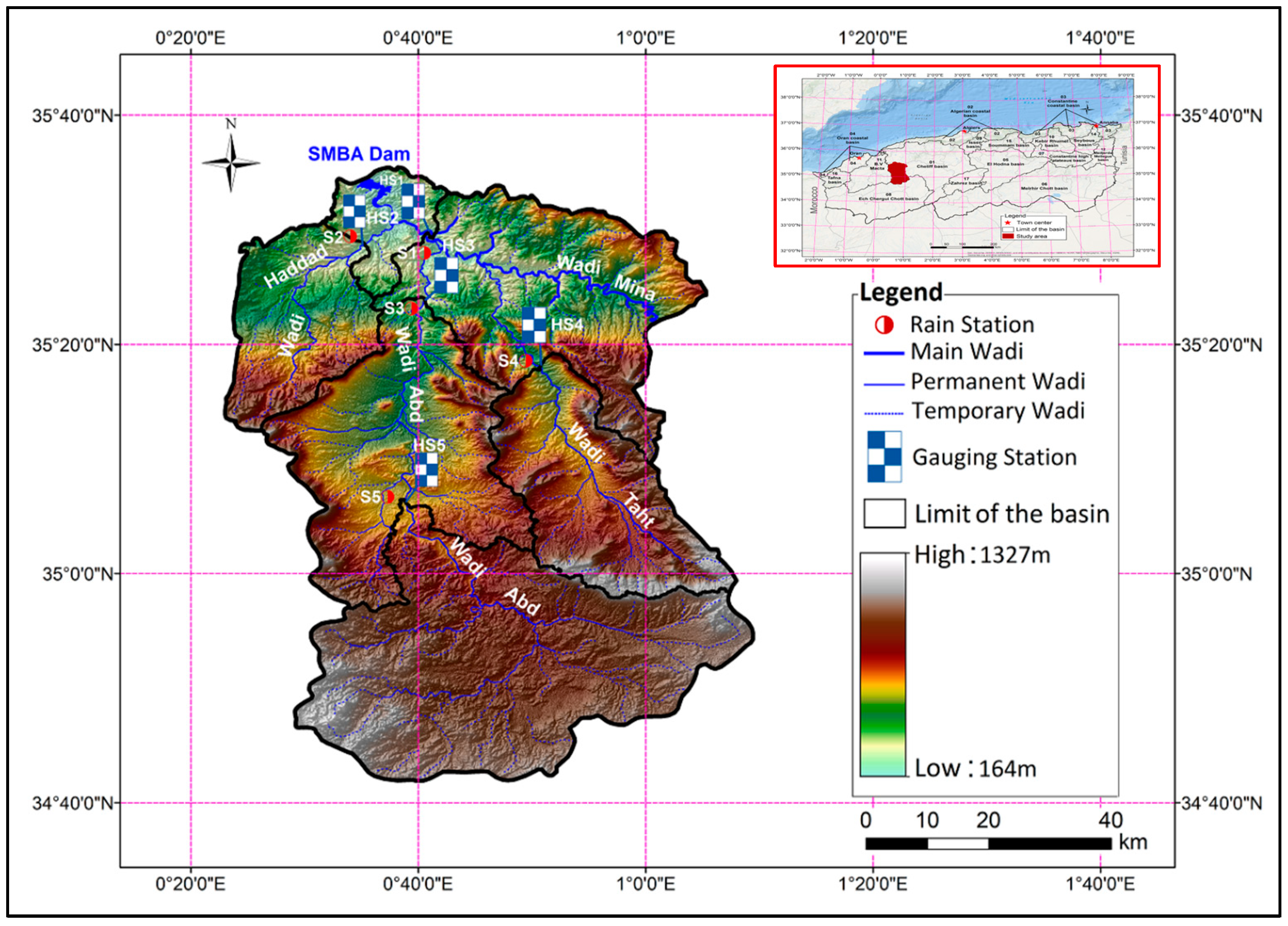
2.1. Study Area and Data

The study region, the Wadi Mina Basin, is located in northwest Algeria (Figure 1). It is located between 00°22′59″ E and 01°09′02″ E and between 34°41′57″ N and 35°35′27″ N. Its area is 4900 km², and its elevation ranges from 164 to 1327 m. The terrain is rugged and complex, and the climate is continental, with significant temperature fluctuations. The main wadi extends 135 km from south to north. Wadi Mina is the principal and final tributary on the left bank of the Wadi Chelif. Its boundaries are the Ouancharis Mountains in the northeast, the Bani Chougrane Mountains in the northwest, the Saida Mountains in the west, the Frenda Mountains in the southeast, and the high plateau in the south. In addition, for vegetation cover, the scrubs make up 32% of the ground vegetation cover, followed by wood and cereal crops at 35.8%. The annual temperature fluctuates between 16 and 19.5 degrees Celsius on average. Most of the 500–250 mm of annual precipitation falls between November and March [22]. For this study, monthly runoff data from five hydrometric stations were collected between 1974 and 2009 by the Agence Nationale des Ressources Hydriques (ANRH) (

Table 1. Characteristics of gauging stations.

ID	Name	Elevation (m)	Basin Area (km2)	Latitude	Longitude
013401	Sidi Abdelkader Djillali	241	480	35°28′46.05″ N	0°35′19.99″ E
013001	Kef Mehboula	502	680	35°18′05.21″ N	0°50′47.89″ E

and Figure 1). Furthermore, the Mann–Whitney test, linear regression, and the double mass curve procedures were used to check the homogeneity of the data and guarantee their quality. The method detected some inhomogeneities, and the erratic data were adjusted with data from reliable adjacent stations [23]. (Table 1 and

Table 2. Training options of the LSTM model.

Parameters of LSTM Model
Number of Features = 1	Max. Epochs = 200	Learning Rate Schedule = piecewise’
Number of Responses = 1	Gradient Threshold = 1	Learn Rate Drop Period = 125
Number of Hidden Units = 200	Initial Learning Rate = 0.005	Learn Rate Drop Factor = 0.2
Train algorithm: Adam	Verbose = 0

and Figure 1).

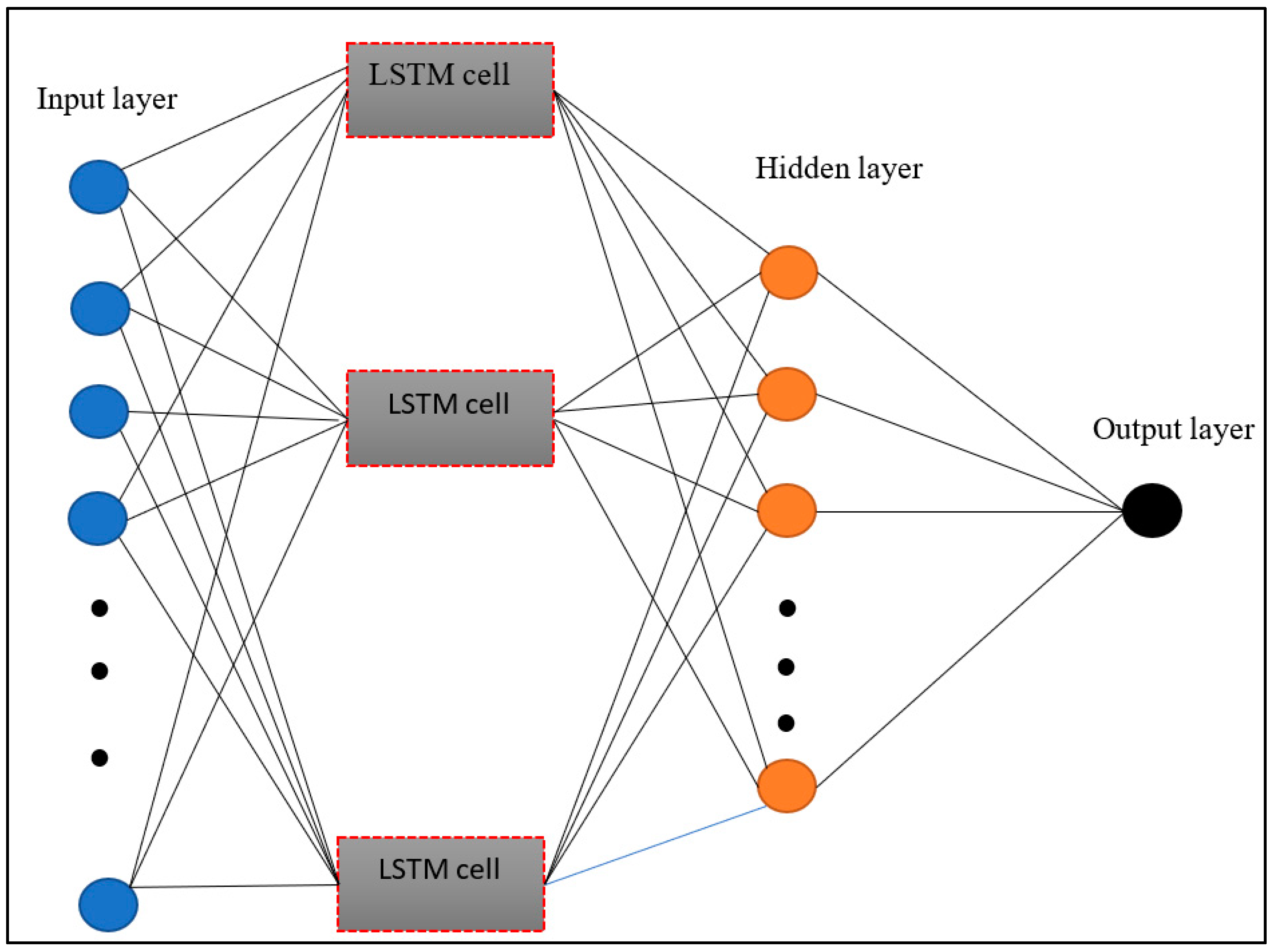
2.2. Long Short-Term Memory (LSTM)

LSTMs represent a significant improvement over RNNs for series forecasting since the method addresses the traditional RNNs’ vanishing gradient problem by integrating gate functions and state dynamics [24,25]. The structure of the LSTM model is presented in Figure 2. The LSTM has memory blocks through layers. Each layer consists of repetitively linked memory cells and forget, input, and output gates [25,26]. The input gate facilitates the addition of information to the cell state as follows: (1) the input values inserted into the cell state are regulated by the sigmoid function, (2) a vector containing all possible values to be inserted into the cell state is generated by the hyperbolic tangent function, and (3) the regulated filter is multiplied by the vector just generated, and the information is inserted into the cell state. The forget gate, which uses a multiplication filter, discards information that is unnecessary for the LSTM to interpret the processes or deemed less significant. The output gate selects relevant information from the present cell state and outputs it.

Assume the input time series data are $x=(x_1, x_2, \dots , x_{t-1}, x_t)$. A typical LSTM cell comprises hyperbolic tangent and sigmoid (σ) layers, along with multiplication ($\times$) and pointwise summation ($+$) operations. It can be used to estimate the target variables $y=(y_1, y_2, \dots , y_{t-1}, y_t)$ by refreshing the gates (output gate $y_t$, forget gate $f_t$, and input gate it) on the memory cell $c_t$, from time t = 1 to T. It is mathematically given below [25,27]:

$$i_t=\sigma (w_i{x}_t+R_i{h}_{t-1}+b_i)$$

(1)

$$f_t=\sigma (w_f{x}_t+R_f{h}_{t-1}+b_f)$$

(2)

$$y_t=\sigma (w_y{x}_t+R_y{h}_{t-1}+b_y)$$

(3)

$$c_t=f_t{c}_{t-1}+i_t{\overline{c}}_t$$

(4)

$${\overline{c}}_t=\sigma (w_c{x}_t+R_c{h}_{t-1}+b_c)$$

(5)

$$h_t=y_t\sigma \left(c_t\right)$$

(6)

The values $b_i$, $b_f$, and by represent bias vectors for the input, forget, and output gates, respectively. The matrices $w_i$, $w_f$, and $w_y$ correspond to the weights connecting the input, forget, and output gates to the input. The vector xt represents the input data, while ht represents the output vector. $R_i$, $R_f$, and $R_y$ indicate the weight matrices from the input, forget, and output gates to the input, respectively. The variables $c_{t-1}$ refer to the previous cell state, and $h_{t-1}$ is the output vector of the previous cell state.

The training parameters of the LSTM model are presented in Table 2. This study uses the LSTM layer with 200 hidden units to train the LSTM model, and the algorithm (adam) is used as the solver. The gradient threshold value was used as 1 to prevent the gradients from bursting. The initial learning coefficient was chosen as 0.005, and after 100 epochs, the learning rate was multiplied by a factor of 0.2.

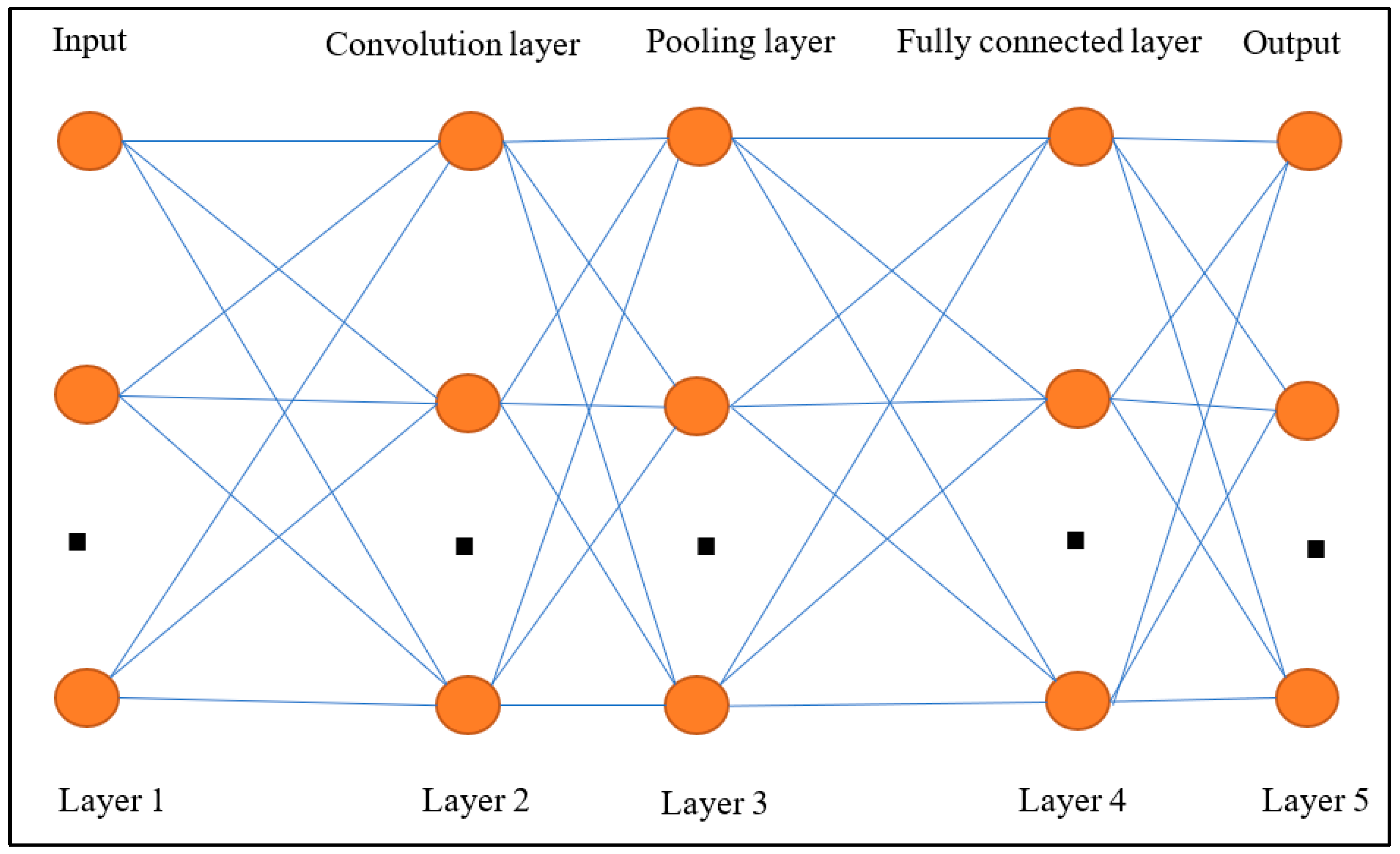
2.3. Convolutional Neural Network (CNN)

The CNN model consists of hidden, input, and output layers. Typically, a 3-D array input is supplied to a convolution layer in which the dimensions are denoted by number of channels, weight, and height. Supposing it is a 1-D input $x={\left(x_t\right)}_{t=0}^{N-1}$ of size N with no zero, the feature output map is produced with the input by a M₁ 3-D filter set, $w_h^1$ for h = 1, …, M₁, where the filters are implemented in the input channels [24,27].

$$a^1\left(i,h\right)=\left(w_h^1\times x\right)\left(i\right)={\sum }_{-\infty }^{+\infty }{w}_h^1\left(j\right)\times (i-j)$$

(7)

in which $a^1\in R^{1\times N-k+1\times M_1}$ represents the output of the first convolutional layer, and $w_h^1\in R^{1\times k\times 1}\mathrm{d}\mathrm{e}\mathrm{n}\mathrm{o}\mathrm{t}\mathrm{e}\mathrm{s}\mathrm{t}\mathrm{h}\mathrm{e}\mathrm{f}\mathrm{i}\mathrm{l}\mathrm{t}\mathrm{e}\mathrm{r}\mathrm{w}\mathrm{e}\mathrm{i}\mathrm{g}\mathrm{h}\mathrm{t}\mathrm{s}$. The resulting feature map then undergoes an activation function h(.), which introduces non-linearity. The output of the first layer is presented as: ${f^1=h(a}^1)$.

The hidden layer contains pooling (PL), convolutional (CL), and fully connected (FCL) layers. The CL automatically extracts features in different regions of the raw input or intermediate feature maps via learnable filters [28]. The filter uses the shared weight matrix to apply the convolution process [29]. The PL turns all values in the pooling window into a single value. Furthermore, the computational cost of the training process is decreased by this layer. This layer addresses any overfitting problem [30].

For the hidden layer $l$ = 2, …, L, the feature map of input $f^{l-1}\in R^{1\times N_{l-1}\times M_{l-1}}$, where $1\times N_{l-1}\times M_{l-1}$ is the size of the output filter map from the previous convolution with $N_{l-1}=N_{l-2}-k+1$, is converted with a set of M₁ filters $w_h^1\in R^{1\times k\times M_{l-1}}$, h = 1, …, M₁, to produce a feature map $a^1\in R^{1\times N_l\times M_l}$ as below [25,28].

$$a^1\left(i,h\right)=\left(w_h^l\times f^{l-1}\right)\left(i\right)={\sum }_{j=-\infty }^{M_{l-1}}{w}_h^1\left(j,m\right)f^{l-1}(i-j,m)$$

(8)

The FCL smooths the high-level deduced features learned by the CL and combines features to gain the final output. The obtained values of feature are then evaluated by passing them through non-linear activation functions $f^1=h\left(a^1\right)$. After CL, the network output will be the matrix $f^L$, whose size is based on the number of filters and filter size utilized in the final layer [25,28]. The structure of the CNN model is presented in Figure 3.

Table 3. Training options of the CNN-RNN model.

Parameters of CNN-RNN Model
Network architecture: CNN-RNN	Horizon = 50	Learning rate = 0.1
Months to look back: 1, 2	Mini Batch Size = 48	Solver: Adam
Train Function = trainlm	Max. Epochs = 250	Momentum constant = 0.25

shows the parameters used in training the CNN-RNN model. Accordingly, the past 1- and 2-months’ time series were used in the streamflow estimation. Levenberg–Marquardt algorithm was used in the training of the network. Levenberg–Marquardt optimization speeds up the error calculation process by applying the least squares method. While training the model, the Adam algorithm was used as a solver. In the setup of the CNN-RNN model, 70% of the streamflow data are reserved for training and testing.

2.4. Recurrent Neural Network (RNN)

LSTM, the recurrent neural network, can explore long-term dependencies among related events over time. It was applied to several topics, such as weather forecasting [31], droughts [32], and solar radiation [33]. The RNN avoids long-term dependencies [24,34], which maintains data in a controller exterior to the normal flow by a new state unit. This memory state block also occurs in a conventional neuron. In the hidden state, the forget gates, output, and input permit RNN to evaluate and check the data flow in isolated chunks, separating two portions known as working memory and memory cells. The memory cell is in charge of the antecedent data from the previous hidden state (i.e., $h_{t-1}$) and new input data, x_t, by the forget gate (g):

$$g_t=\sigma (w_g\times \left[h_{t-1},x_t\right]+b_g)$$

(9)

in which the working memory (h_t) is utilized as an output gate to govern the proportion of the current memory c_t. ${\tilde{c}}_t$ is an updated state generated by $x_t$ and $h_{t-1}$ with the help of tanh layer. It can be written as follows:

$$j_t=\rho (v_j\times \left[h_{t-1},x_t\right]+{\phi }_j)$$

(10)

$${\tilde{c}}_t=tanh(v_c\times \left[h_{t-1},x_t\right]+{\phi }_c)$$

(11)

Both $c_{t-1}$ and c_t are obtained in the forget gate (g) and input gate (j), as follows:

$$c_t=g_t\times c_{t-1}+i_t\times {\tilde{c}}_t$$

(12)

There are two stages involved in processing the output. The output gate, known as a novel gate, determines the relevant components. The c_t state is activated using the tanh function and then adjusted by multiplying it with the obtained $o_t$ to produce the desired output ht. In other words, the output gate helps select the relevant information, while the c_t state is modified and combined with the output gate to generate the final output h_t.

$$o_t=\sigma (v_0\times \left[h_{t-1},x_t\right]+b_0)$$

(13)

$$h_t=o_t\times tanhh\left(c_t\right)$$

(14)

in which $\rho \left(\right)$ is the sigmoid activation function, ${\phi }_g, {\phi }_j, {\phi }_c, {\phi }_0$ are bias vectors, and $v_g, v_j, v_c, v_0$ are weight matrices.

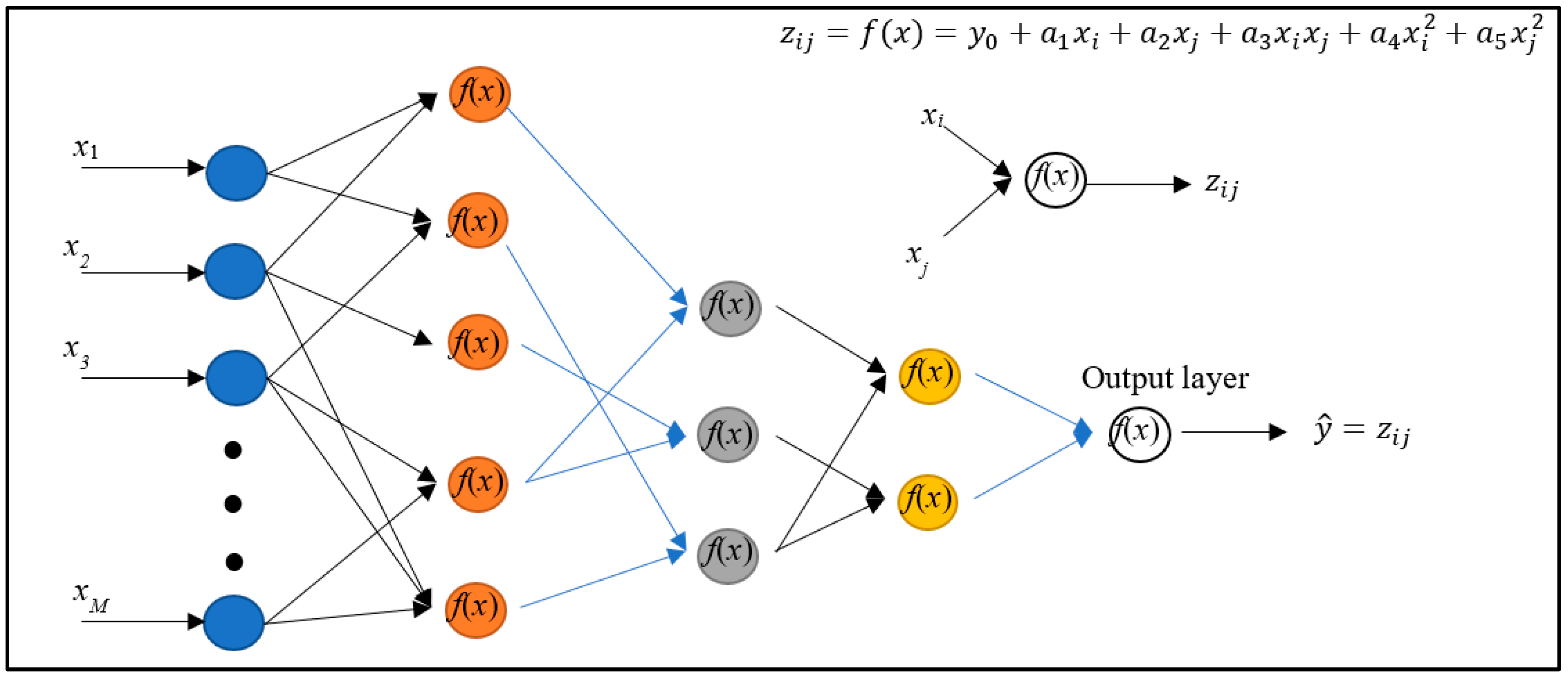
2.5. The Group Method of Data Handling Model (GMDH)

The GMDH algorithm was pioneered by Ivakhnenko [35] to set models and identify complex systems. It was defined to obtain higher-order regression polynomials for solving problems related to modeling and classification. The inputs and output variables can be clarified by complex polynomial series by the Volterra series, called the Kolmogorov–Gabor polynomial [35]:

$$y=a_0+{\sum }_{i=1}^M{a}_i{x}_i+{\sum }_{i=1}^M{\sum }_{j=1}^M{a}_{ij}{x}_i{x}_j+{\sum }_{i=1}^M{\sum }_{j=1}^M{\sum }_{k=1}^M{a}_{ijk}{x}_i{x}_j{x}_k+\dots$$

(15)

where x is the system’s input, M is the number of inputs, and a is the coefficients or weights.

$$y=y_0+a_1{x}_i+a_2{x}_j+a_3{x}_i{x}_j+a_4{x}_i^2+a_5{x}_j^2$$

(16)

The Gauss normal equation is resolved to acquire a value for each m model. The a_i of nodes in each layer are defined as below:

$$A={\left(X^{T}X\right)}^{-1}{X}^{T}Y$$

(17)

where

$$Y={\left[y_1{y}_2\dots y_M\right]}^T,A=[a_0,a_1,a_2,a_3,a_4,a_5]$$

(18)

$$\left[\begin{array}{cccccc}1& x_{1p}& x_{1q}& x_{1p}{x}_{1q}& x_{1p}^2& x_{1q}^2\\ 1& x_{2p}& x_{2q}& x_{2p}{x}_{2q}& x_{2p}^2& x_{2q}^2\\ ⋮& ⋮& ⋮& ⋮& ⋮& ⋮\\ 1& x_{Mp}& x_{Mq}& x_{Mp}{x}_{Mq}& x_{Mp}^2& x_{Mq}^2\end{array}\right]$$

(19)

where M represents the count of real values. The primary function of GMDH relies on the forward propagation of the signal through nodes, akin to neural networks. Each layer comprises elementary nodes that relay the output to the nodes in the succeeding layer as shown in Figure 4. The fundamental steps involved in conventional GMDH modeling are as follows [36,37]. The following guidelines involve (1) selecting normalized data X = {x₁, x₂, …, x_M} as input variables and separating data into training and testing data sets; (2) setting ^MC₂ = M(M − 1)/2 new variables in the training data set and the regression polynomial for first layer by forming the quadratic expression, which is nearly equal to the output (y) in Equation (16); (3) identifying the contributing nodes at each hidden layer by analyzing error values and replacing the least useful variable with new columns of Z in place of old columns (X); (4) conducting this process by repeating steps (2) and (3). The iterative computation is finalized if the test data errors in each layer do not decrease.

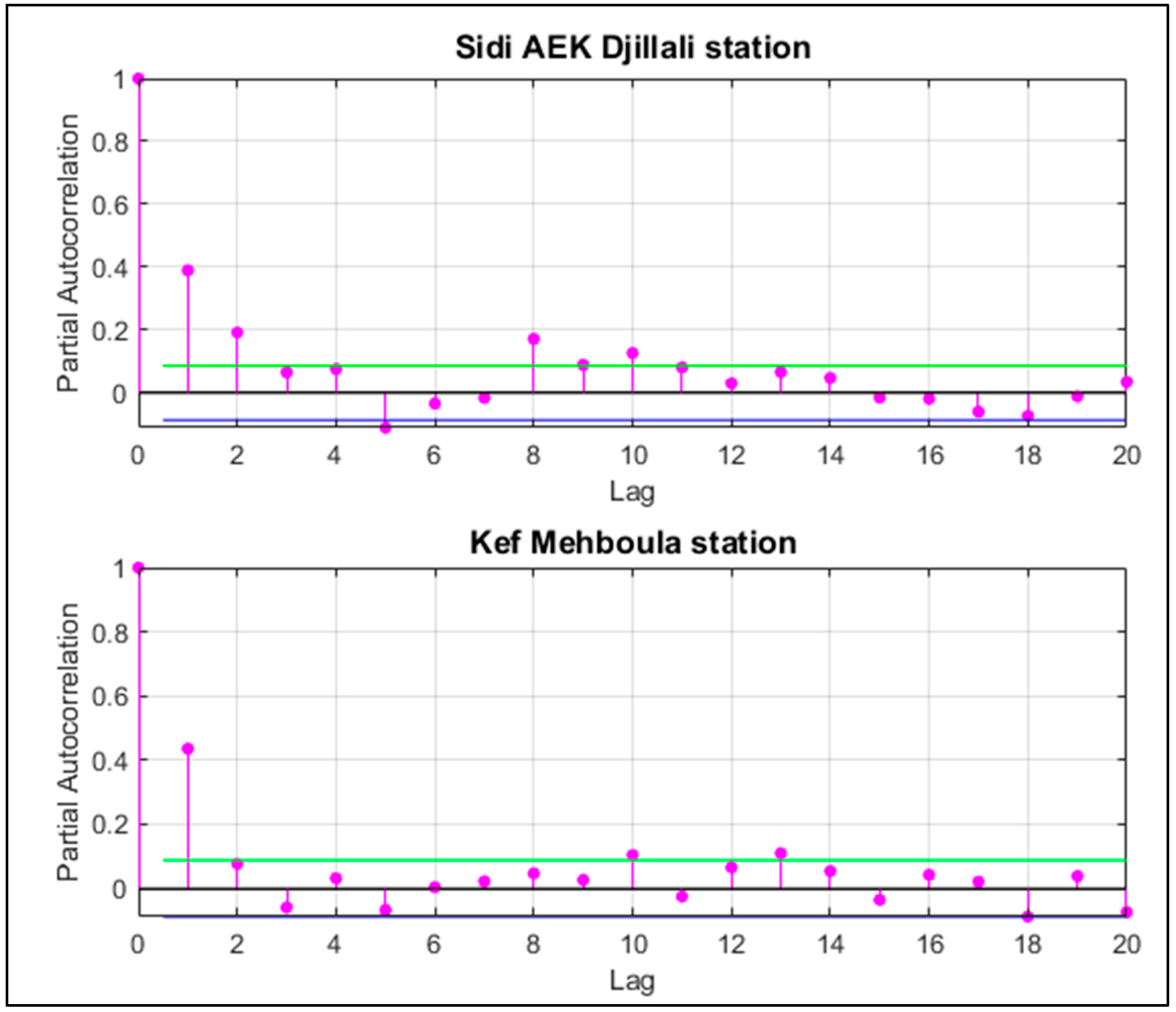
2.6. Selection of Model Input Combinations

PACF graphs of streamflow values are presented in Figure 5. The delayed streamflow values of these graphs exceeding the confidence limit are presented as input to the models. Accordingly, streamflow values with a delay of 2 months at Sidi Abdelkader Djillali station and a delay of 1 month for Kef Mehboula station were presented as inputs to the AI models. This study used newly developed LSTM, CNN-RNN, and GMDH techniques to compare the performance of DL and ML approaches in estimating monthly streamflow values. In the setup of the models, 70% of the data were chosen as training and the rest as testing. Partial autocorrelation graphs (PACF) were used to select model input combinations. The performances of the established models were compared according to MSE, MAE, MBE, and R values.

2.7. Measurement of Model Prediction Success

The preciseness of LSTM, CNN, RNN, GMDH, and CNN-RNN models was assessed via some statistical metrics to forecast the streamflow. This study used four different statistical metrics to compare the estimation performance of streamflow prediction. The models’ performance was assessed with mean square error (MSE), mean absolute error (MAE), mean bias error (MBE), and the correlation coefficient (R). MSE represents the mean square errors between the predicted values and the true values. This metric is an effective tool for evaluating the overall performance of the model because it penalizes large errors more. MAE calculates the mean of the absolute values of the differences between the predicted values and the observations. This metric makes it easier to interpret the magnitude of the errors and prevents positive or negative errors from canceling each other out. Small error values indicate the accuracy and consistency of the models. MBE is a metric used to detect systematic errors in the model. It determines the tendency of the predicted values to deviate from the observations (positive or negative). A positive MBE indicates that the model generally overestimates the values; a negative MBE indicates that it underestimates the values. The correlation coefficient measures the linear relationship between the predicted and observed values. An R value close to 1 indicates that the model represents the observations with high accuracy. This metric is important in understanding the strength of the relationship between variables, as well as evaluating the overall accuracy of the predictions. Equations of statistical metrics are commonly interpreted in several studies [25,38]. R is the linear regression strength between actual and estimated values. The relationship is the strongest when R = 1. The MAE and MSE provide information about the preciseness of the models. The following equations materialize when employed to derive these metrics.

$$\mathrm{R}=\sqrt{{\displaystyle \frac{{\sum }_{i=1}^n{\left(o_i-o_{mean}\right)}^2-{\sum }_{i=1}^n{\left(o_i-p_i\right)}^2}{{\sum }_{i=1}^n{\left(o_i-o_{mean}\right)}^2}}}$$

(20)

$$\mathrm{M}\mathrm{S}\mathrm{E}={\displaystyle \frac{1}{N}}{\sum }_{i=1}^n{{(p}_i-o_i)}^2$$

(21)

$$\mathrm{M}\mathrm{A}\mathrm{E}={\displaystyle \frac{1}{N}}{\sum }_{i=1}^n\left|\left(p_i-o_i\right)\right|$$

(22)

$$\mathrm{M}\mathrm{B}\mathrm{E}={\displaystyle \frac{1}{N}}{\sum }_{i=1}^n\left(p_i-o_i\right)$$

(23)

in which o is the actual value, and p is the predicted value; o_i and p_i are the actual and predicted ith value. Error values near 0 and R show the most accurate estimation results.

3. Results

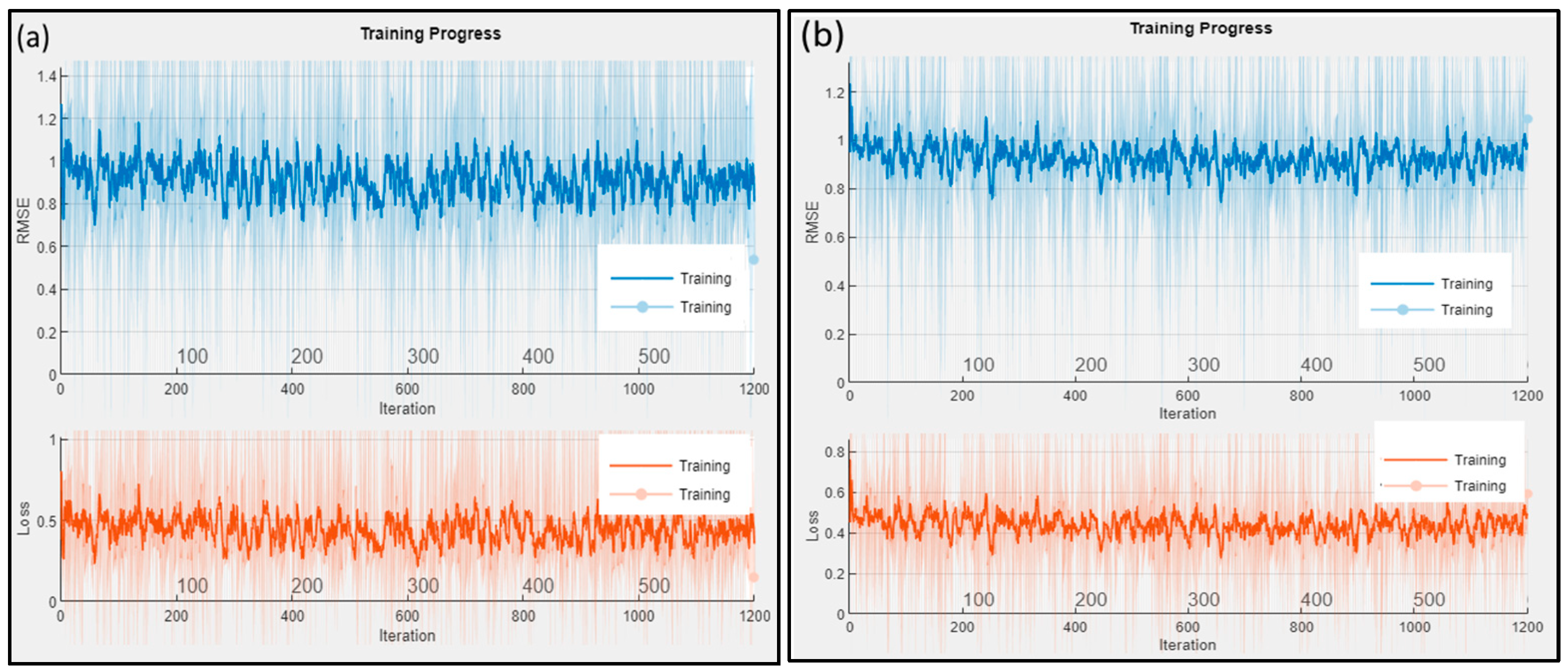
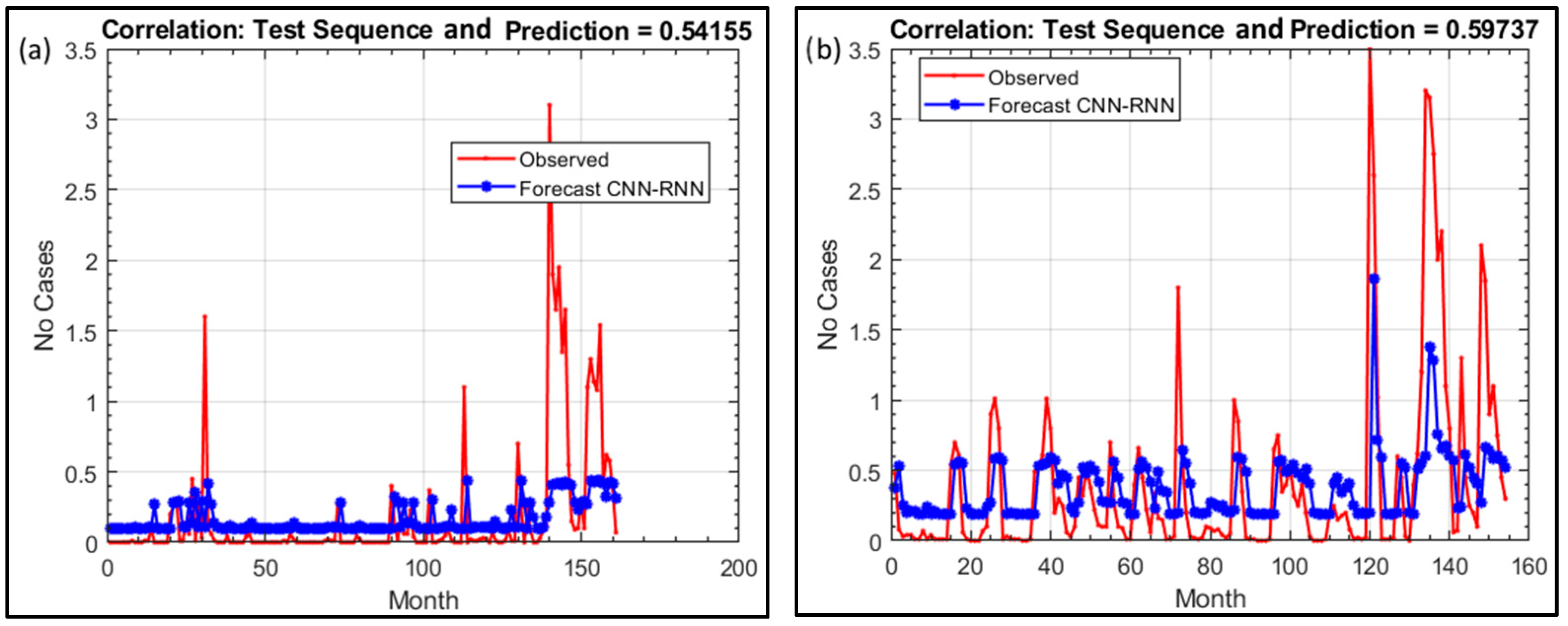
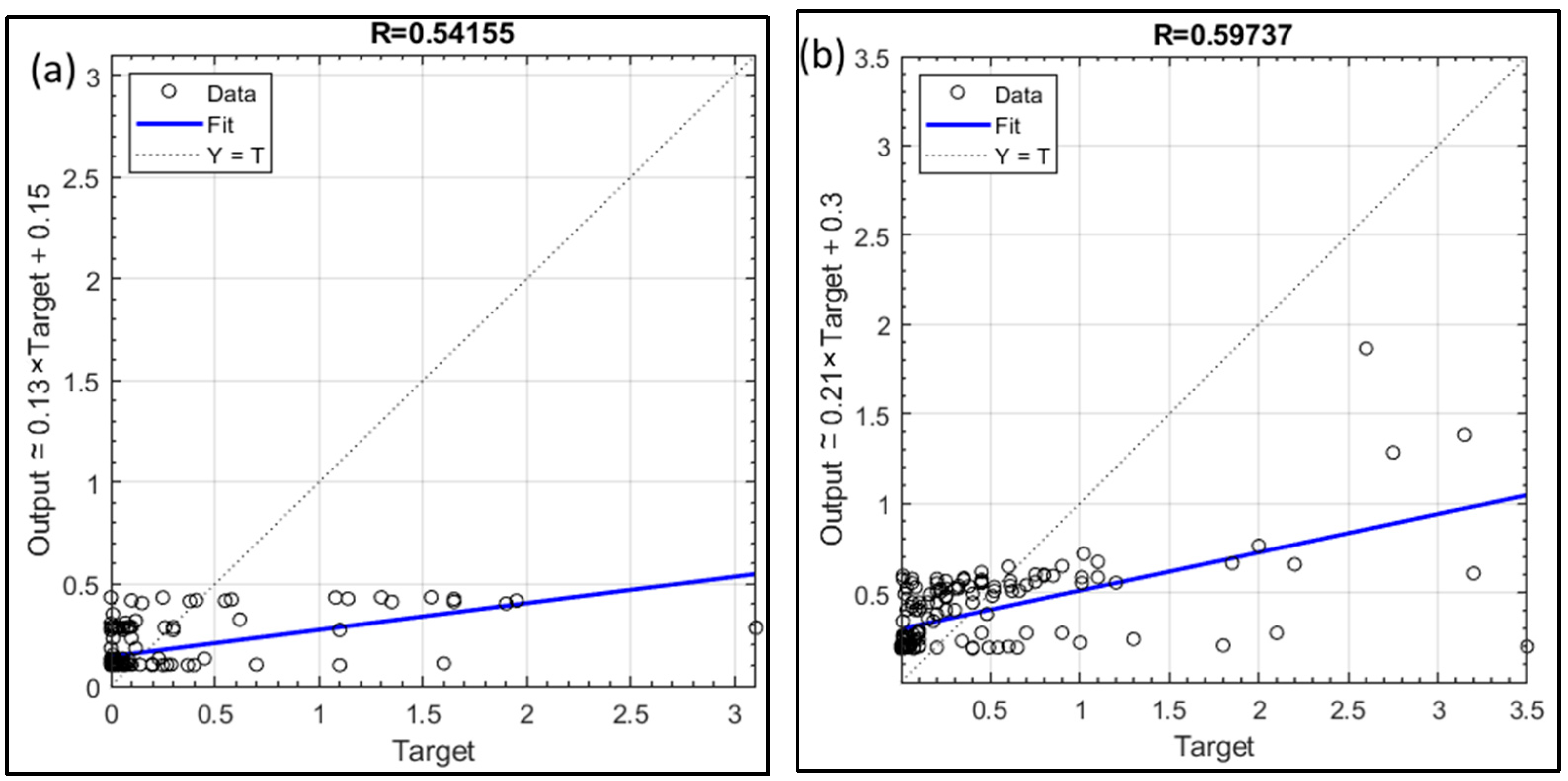
3.1. CNN-RNN Results

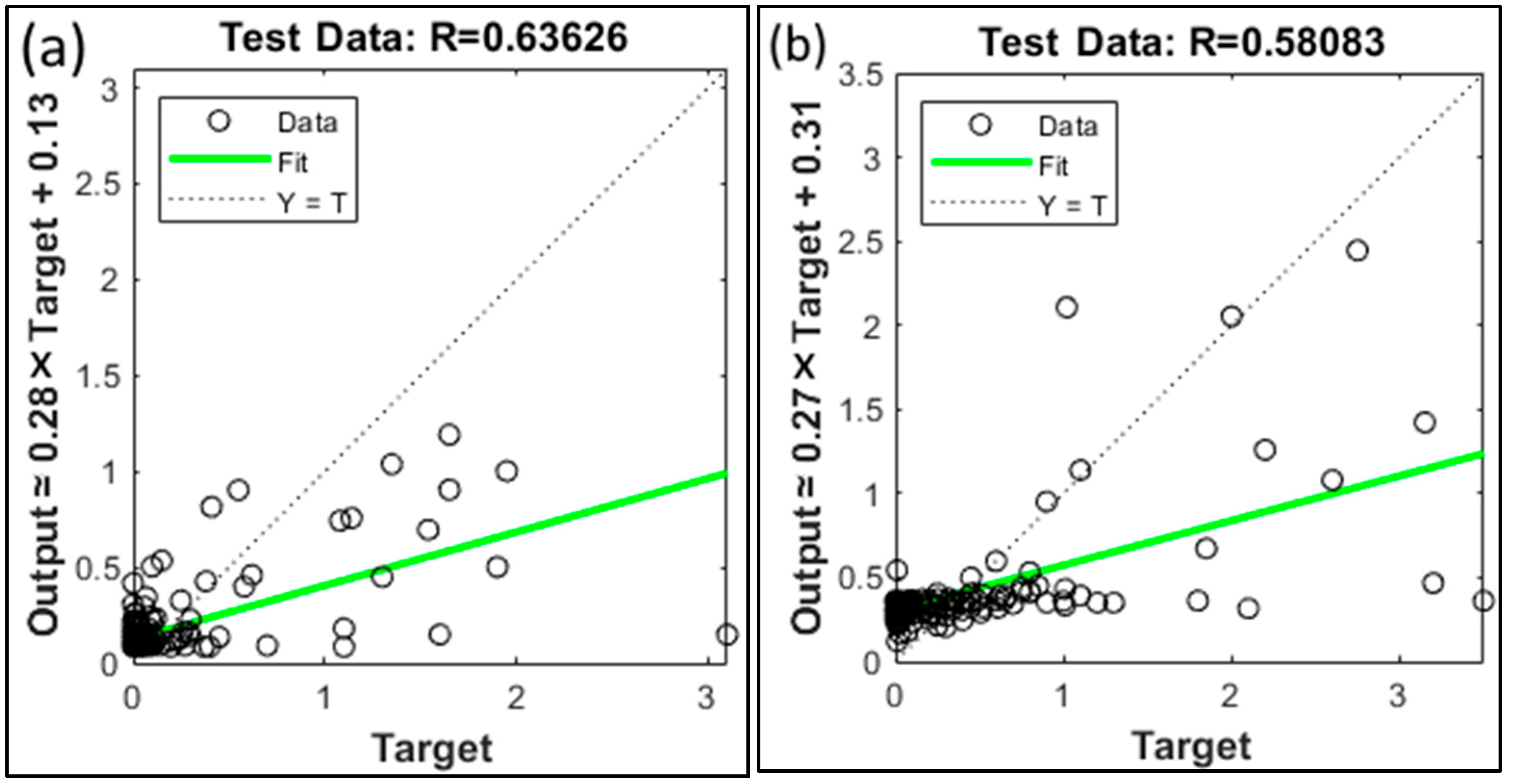
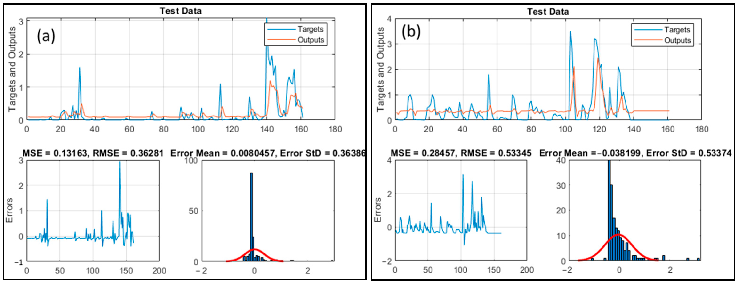
In this part of the study, extreme flow values were estimated by combining CNN and RNN. The previous 1- and 2-month data were used as input to the model. In this approach, the CNN algorithm was utilized for feature extraction, and RNN was employed to estimate streamflow values. MATLAB 2019a was used to develop all models.

Convolutional layers reveal the local characteristics of the data by shifting the inputs using filters. Pooling layers reduce the size of the data and allow features to be expressed more generally, thus enhancing the success of the model. RNN is an effective approach for capturing temporal or serial dependencies of data. As a result, the future situation can be modeled based on past data. Figure 6 shows the training development of the CNN-RNN-based streamflow prediction model constructed at Sidi AEK Djillali and Kef Mehboula stations. As shown in the Figure 6, with the increase in the number of iterations, the error values and loss values decrease, indicating the model’s successful training.

In Figure 7, streamflow time series in the test phase are compared to show the performance of the CNN-RNN algorithm. Accordingly, it is seen that generally close estimates are obtained at the Sidi AEK Djillali station, except for the peak values. In addition, estimation results more comparable to reality are obtained at Kef Mehboula station than at other stations. However, peak values could not be estimated. For this reason, the models’ performances are generally seen as poor. The near-zero streamflow values can explain this situation due to droughts in the basin.

Figure 8 shows the scatter diagrams of the CNN-RNN model during the testing phase. Accordingly, although the data at Sidi AEK Djillali station are far from the regression line, the data at Kef Mehboula station approach the regression line a little. In addition, the correlation coefficients of the models are 0.54 at Sidi AEK Djillali station, while it is around 0.60 at Kef Mehboula station. When the actual and estimation data are examined, the flow values above 1 cannot be estimated well. However, other values have been estimated quite successfully.

3.2. GMDH Results

During the training of the GMDH model, Maximum Number of Neurons in a Layer: 25, Maximum Number of Layers: 5, and Selection Pressure: 0 were used. Figure 9a,b show the scattering diagram of the test results obtained at Sidi AEK Djillali and Kef Mehboula stations, respectively. Accordingly, although the dead are generally gathered around the regulation line, it is noteworthy that the deviations increase as the data values increase.

In Figure 10, streamflow time series in the testing phase are presented to evaluate the performance of the GMDH algorithm in stream estimation. Accordingly, it is seen that the streamflow values at Sidi AEK Djillali station are quite close to reality. At Kef Mehboula station, it is seen that it cannot predict the maximum and minimum values. However, it is seen that it predicts the current values close to the mean quite satisfactorily. In addition, when the error intakes are examined, it has been determined that the models generally perform poorly in the pih values. In addition, as can be seen from the histogram graphs of the errors, the errors conform to the normal distribution.

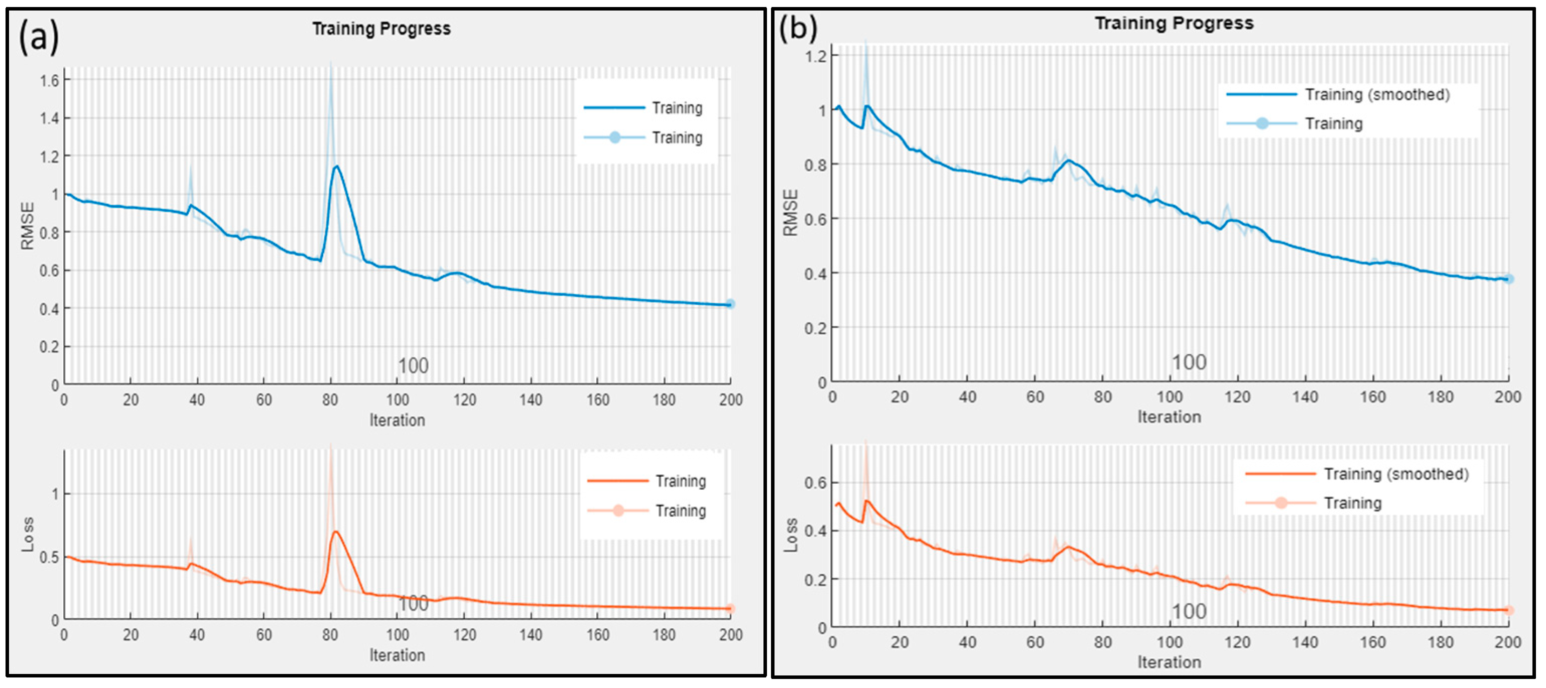
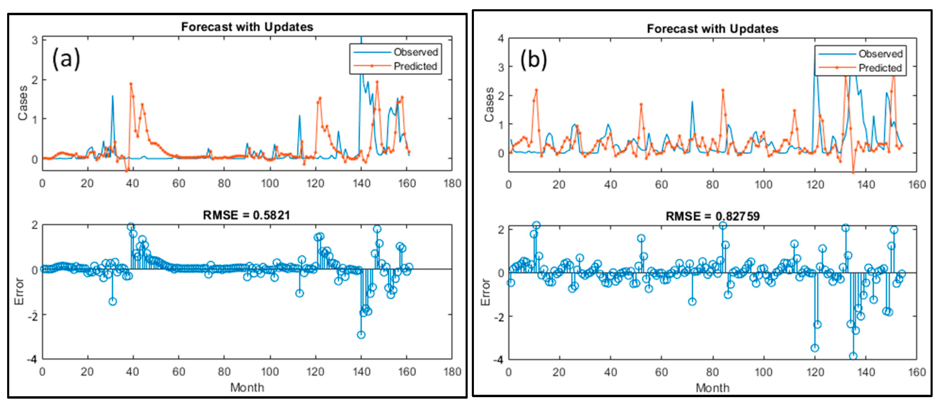
3.3. LSTM Model Results

The LSTM network is a network that processes input data and updates the RNN state. The RNN state is able to use the information remembered at all previous time steps. In this study, the previous streamflow data time steps are presented to the LSTM model, and the time series’ next values are estimated.

Figure 11 shows the training phase of the LSTM model at the Sidi AEK Djillali station. Accordingly, it is seen that the prediction error of the model decreases as the number of iterations increases. A total of 200 iterations were used in the model setup. In addition, it was emphasized that the training phase was carried out effectively since the errors became quite horizontal after the 160th iteration. In Figure 11b, the training phase of the LSTM model at the Kef Mehboula station is presented. In streamflow time series estimation with the LSTM network, at each time step of the input sequence, it tries to predict the value of the next time step. It predicts steps one by one by updating the state of the network and using the predictAndUpdateState function on each prediction. When the training error propagation is evaluated, it is seen that the error values continue to move in a fairly horizontal state after the 180th iteration. This indicates the adequacy of training.

The state of the network is updated according to the predicted and observed values. The network is reset with the resetState command to evaluate the current estimation accuracy. Thus, the predictive success of the network is tested. In Figure 12, the accuracy of the LSTM algorithm is evaluated in estimating flow stream time series in the test phase. Accordingly, both stations generally showed poor prediction performance, except for the minimum values. In addition, significant deviations from the actual current values were observed in both stations, especially at the maximum current values.

3.4. Evaluation of the Performance of Models

Various statistical values were examined to compare the performances of DL and ML models. Accordingly, the lowest error values (MSE, MAE, and MBE) and the closest correlation (R) values to 1 indicate the optimum model. The performance outputs of the DL and ML models established in

Table 4. Model performance evaluation.

	MSE	MAE	MBE	R
Sidi AEK Djillali station
LSTM	0.339	0.317	0.053	0.102
CNN-RNN	0.166	0.217	−0.017	0.542
GMDH	0.132	0.185	−0.008	0.636
Kef Mehboula station
LSTM	0.685	0.489	−0.041	0.039
CNN-RNN	0.298	0.335	−0.018	0.597
GMDH	0.285	0.349	0.038	0.581

Note: Bold terms indicate the optimum model.

are presented. Accordingly, while the most accurate results were obtained according to the GMDH model at Sidi AEK Djillali station, high errors were observed in the LSTM model. In addition, while the most accurate current estimation was made with the CNN-RNN model at Kef Mehboula station, the weakest estimation performance was obtained with the LSTM model.

The superior performance of the GMDH model may be due to its ability to establish relationships in data sets with complex characteristics. This model works on the principle of iteratively deriving polynomials that explain the relationship with the data. The low MSE (0.132) and MAE (0.185) values at Sidi AEK Djillali station may have enabled the model to produce results that are compatible with the observations. In the learning process of GMDH, model complexity is optimized by selecting appropriate polynomials. Data density and distribution at Sidi AEK Djillali and Kef Mehboula stations may affect the model performance. It can be thought that the data at Sidi AEK Djillali station have a more balanced distribution and, therefore, GMDH provides superior performance. The low error values at Sidi AEK Djillali station indicate that the hydrological data structure of this station can be highly compatible with the mathematical approach of GMDH. GMDH provides effective results on missing data or non-linear relationships between variables. The higher correlation coefficient (R = 0.636) at this station supports that the model establishes a correct relationship with the station data.

4. Discussion

This study aims to predict the monthly streamflow time series using LSTM, CNN-RNN, and GMDH algorithms. For this purpose, the effect of AI and DL algorithms on monthly streamflow forecasting performance was analyzed.

Dehghani et al. [39] used convolutional LSTM (ConvLSTM), LSTM, and convolutional neural network (CNN) models to predict short-term current. They found that these models predicted short-term flow with high accuracy; the LSTM model performed better in small basins with well-spatially distributed precipitation stations, while ConvLSTM and CNN models were more effective in medium to high flows and large river basins. The findings obtained from the study by Dehghani et al. [39] overlap in terms of the fact that the CNN and LSTM models used are the same, and the CNN model provides good results. However, these findings do not overlap because the short-term flow estimation was used in the study.

Forghanparast and Mohammadi [9] used LSTM, CNN, and Self-Attention LSTM (SA-LSTM) algorithms to predict monthly flows and compared them to the basic extreme learning machine (ELM) model. As a result, they determined that LSTM-based models from DL algorithms showed higher accuracy and better stability than ELM. The results of this study coincide with Forghanparast and Mohammadi’s [9] monthly flow estimation study in establishing models such as CNN and LSTM algorithm, but not in terms of LSTM-based models giving better results. This may be due to the arid climate of the study area. Khodakhah et al. [40] investigated ANFIS, seasonal autoregressive integrated moving average (SARIMA), least squares support vector machine (LSSVM), and GMDH algorithms to forecast the monthly streamflow, and they determined that the GMDH algorithm gave the best results among the ML algorithms. The findings obtained from the study overlap with the study of Khodakhah et al. [40] in that the GMDH algorithm produces one of the most effective results in monthly flow estimation.

Ghimire et al. [41] used the CNN-LSTM hybrid model derived from LSTM and CNN models to predict short-term hourly streamflow. Their results showed that the proposed hybrid CNN-LSTM model achieved highly accurate short-term predictions with significant practical value. This study overlaps with the analysis of the use of CNN and LSTM models in flow forecasting in the study of Ghimire et al. [41] but differs fundamentally due to the use of short-term hourly flow forecasting. Additionally, the reliable results of the CNN-RNN hybrid model in this study align with the robust performance of the CNN-LSTM hybrid model.

Cheng et al. [42] researched the LSTM and ANN algorithms to predict daily and monthly flow over a long preparation period. It has been determined that the LSTM algorithm gives better results than the ANN algorithm in daily flow prediction, while it gives bad results in monthly flow forecasting. This study coincides with the poor results obtained from the LSTM model in the study of Cheng et al. [42] used in monthly flow estimation. Sahoo et al. [43] used the LSTM-recurrent neural network (LSTM-RNN) hybrid model to forecast the low-streamflow time series. They found that LSTM-RNN is a reliable algorithm for low-current estimation. The findings obtained from the study of Sahoo et al. [43] overlap in terms of the estimation of long-term low currents and the reliable results of the hybrid models used. However, different hybrid models based on RNN were used in both studies.

As a result of the estimation analysis of the algorithms used in the study, although the researched region is an arid region, it has been concluded that AI and DL algorithms allow the monthly streamflow time series forecasts to be used effectively and reliably. The results of Dehghani et al. [39], Khodakhah et al. [40], Forghanparast and Mohammadi [9], Ghimire et al. [41], Cheng et al. [42], and Sahoo et al. [43] in the literature are compatible with the presented research. Furthermore, Tian et al. [44,45] suggested that an ensemble method utilizing multiple deep learning (DL) algorithms exhibits greater robustness than individual DL algorithms in forecasting atmospheric rivers; this hypothesis will be evaluated in our subsequent research on streamflow prediction.

5. Conclusions

In this study, the accuracy of three AI algorithms is compared while predicting monthly streamflow time series at the Sidi AEK Djillali and Kef Mehboula stations: the LSTM, CNN-RNN, and GMDH. Mean square error (MSE), mean absolute error (MAE), mean bias error (MBE), and the correlation coefficient (R) are the four metrics used to evaluate the performance of the models. The results of the research are expressed as follows:

• At the Sidi AEK Djillali station, the GMDH model outperformed both the LSTM and CNN-RNN models across all four evaluation metrics.
• The GMDH model registered MSE and MAE values of 0.132 and 0.185, respectively, highlighting its enhanced predictive accuracy. Its R value of 0.636 demonstrates strong alignment with observed data, and its minimal MBE of −0.008 indicates reduced bias.
• At the Kef Mehboula station, the GMDH and CNN-RNN models outperformed the LSTM model. The CNN-RNN model had the most favorable MSE value of 0.285, while the GMDH model performed best in MAE, scoring 0.335. Both models exhibited strong correlation coefficients with observed data, with R values of 0.581 and 0.597, respectively.
• The GMDH model showed a modest overestimation with a positive MBE (0.038). Overall, the GMDH model performed best at both stations, but all three models demonstrated promise for predicting monthly streamflow time series.

Future research could incorporate additional climate variables into the models to enhance the precision and comprehensiveness of predictions. Additionally, assessing these models in diverse geographical settings may provide insights into their broader applicability across hydrological conditions. Moreover, extending model inputs to include high-resolution remote sensing data (e.g., radar rainfall estimates or satellite-derived soil moisture) could further enhance the fidelity of the simulations. Evaluating the performance of the models under extreme hydro-climatic scenarios (e.g., flash floods or prolonged droughts) may also uncover critical thresholds and guide risk-based water resource management. In addition, implementing advanced hyperparameter optimization methods (e.g., genetic algorithms or adaptive learning rates) could lead to faster convergence and more stable prediction outcomes, particularly in large-scale applications.

References

1. Mehdizadeh, S.; Kozekalani Sales, A. A Comparative Study of Autoregressive, Autoregressive Moving Average, Gene Expression Programming and Bayesian Networks for Estimating Monthly Streamflow. Water Resour. Manag. 2018, 32, 3001–3022. [Google Scholar] [CrossRef]
2. Al-Juboori, A.M. A Hybrid Model to Predict Monthly Streamflow Using Neighboring Rivers Annual Flows. Water Resour. Manag. 2021, 35, 729–743. [Google Scholar] [CrossRef]
3. Zhu, S.; Luo, X.; Yuan, X.; Xu, Z. An improved long short-term memory network for streamflow forecasting in the upper Yangtze River. Stoch. Environ. Res. Risk Assess. 2020, 34, 1313–1329. [Google Scholar] [CrossRef]
4. Yaseen, Z.M.; Fu, M.; Wang, C.; Mohtar, W.H.M.W.; Deo, R.C.; El-Shafie, A. Application of the Hybrid Artificial Neural Network Coupled with Rolling Mechanism and Grey Model Algorithms for Streamflow Forecasting Over Multiple Time Horizons. Water Resour. Manag. 2018, 32, 1883–1899. [Google Scholar] [CrossRef]
5. Samanataray, S.; Sahoo, A.A. Comparative Study on Prediction of Monthly Streamflow Using Hybrid ANFIS-PSO Approaches. KSCE J. Civ. Eng. 2021, 25, 4032–4043. [Google Scholar] [CrossRef]
6. Shu, X.; Ding, W.; Peng, Y.; Wang, Z.; Wu, J.; Li, M. Monthly Streamflow Forecasting Using Convolutional Neural Network. Water Resour. Manag. 2021, 35, 5089–5104. [Google Scholar] [CrossRef]
7. Lin, Y.; Wang, D.; Wang, G.; Qiu, J.; Long, K.; Du, Y.; Dai, Y.; Xie, H.; Wei, Z.; Shangguan, W.; et al. A hybrid deep learning algorithm and its application to streamflow prediction. J. Hydrol. 2021, 601, 126636. [Google Scholar] [CrossRef]
8. Khosravi, K.; Golkarian, A.; Tiefenbacher, J.P. Using Optimized Deep Learning to Predict Daily Streamflow: A Comparison to Common Machine Learning Algorithms. Water Resour. Manag. 2022, 36, 699–716. [Google Scholar] [CrossRef]
9. Forghanparast, F.; Mohammadi, G. Using Deep Learning Algorithms for Intermittent Streamflow Prediction in the Headwaters of the Colorado River, Texas. Water 2022, 14, 2972. [Google Scholar] [CrossRef]
10. Haznedar, B.; Kilinc, H.C.; Ozkan, F.; Yurtsever, A. Streamflow forecasting using a hybrid LSTM-PSO approach: The case of Seyhan Basin. Nat. Hazards 2023, 117, 681–701. [Google Scholar] [CrossRef]
11. Katipoğlu, O.M. Monthly streamflow prediction in Amasya, Türkiye, using an integrated approach of a feedforward backpropagation neural network and discrete wavelet transform. Model. Earth Syst. Environ. 2023, 9, 2463–2475. [Google Scholar] [CrossRef]
12. Katipoğlu, O.M.; Keblouti, M.; Mohammadi, B. Application of novel artificial bee colony optimized ANN and data preprocessing techniques for monthly streamflow estimation. Environ. Sci. Pollut. Res. 2023, 30, 89705–89725. [Google Scholar] [CrossRef]
13. Abda, Z.; Zerouali, B.; Chettih, M.; Santos, C.A.G.; de Farias, C.A.S.; Elbeltagi, A. Assessing machine learning models for streamflow estimation: A case study in Oued Sebaou watershed (Northern Algeria). Hydrol. Sci. J. 2022, 67, 1328–1341. [Google Scholar] [CrossRef]
14. Tikhamarine, Y.; Souag-Gamane, D.; Mellak, S. Stream flow prediction using a new approach of hybrid artificial neural network with discrete wavelet transform. A case study: The catchment of Seybouse in northeastern Algeria. Alger. J. Environ. Sci. Technol. 2022, 8, 2435–2439. [Google Scholar]
15. Beddal, D.; Achite, M.; Baahmed, D. Streamflow prediction using data-driven models: Case study of Wadi Hounet, northwestern Algeria. J. Water Land Dev. 2020, 47, 16–24. [Google Scholar] [CrossRef]
16. Karakoyun, E.; Kaya, N. Hydrological simulation and prediction of soil erosion using the SWAT model in a mountainous watershed: A case study of Murat River Basin, Turkey. J. Hydroinf. 2022, 24, 1175–1193. [Google Scholar] [CrossRef]
17. Mehr, A.D.; Ghadimi, S.; Marttila, H.; Haghighi, A.T. A new evolutionary time series model for streamflow forecasting in boreal lake-river systems. Theor. Appl. Climatol. 2022, 148, 255–268. [Google Scholar] [CrossRef]
18. Atashi, V.; Gorji, H.T.; Shahabi, S.M.; Kardan, R.; Lim, Y.H. Water level forecasting using deep learning time-series analysis: A case study of red river of the north. Water 2022, 14, 1971. [Google Scholar] [CrossRef]
19. Kartal, V.; Karakoyun, E.; Akiner, M.E.; Katipoğlu, O.M.; Kuriqi, A. Optimizing river flow rate predictions: Integrating cognitive approaches and meteorological insights. Nat. Hazards 2024, 1–28. [Google Scholar] [CrossRef]
20. Roniki, A.; Swain, R.; Behera, M.D. Future projections of worst floods and dam break analysis in Mahanadi River Basin under CMIP6 climate change scenarios. Environ. Monit. Assess. 2023, 195, 1173. [Google Scholar]
21. Fatemeh, G.; Kang, D. Improving long-term streamflow prediction in a poorly gauged basin using geo-spatiotemporal mesoscale data and attention-based deep learning: A comparative study. J. Hydrol. 2022, 615, 128608. [Google Scholar]
22. Achite, M.; Touaibia, B. Sécheresse et gestion des ressources en eau dans le bassin versant de la Mina. In Proceedings of the 2ème Colloque International Sur L’eau et L’Environnement, Sidi Fredj, Algérie, 30 January 2007. [Google Scholar]
23. Achite, M.; Wałęga, A.; Toubal, A.K.; Mansour, H.; Krakauer, N. Spatiotemporal characteristics and trends of meteorological droughts in the wadi mina basin, northwest algeria. Water 2021, 13, 3103. [Google Scholar] [CrossRef]
24. Hochreiter, S.; Schmidhuber, J. Long short-term memory. Neural Comput. 1997, 9, 1735–1780. [Google Scholar] [CrossRef]
25. Barzegar, R.; Aalami, M.T.; Adamowski, J. Short-term water quality variable prediction using a hybrid CNN–LSTM deep learning model. Stoch. Environ. Res. Risk Assess. 2020, 34, 415–433. [Google Scholar] [CrossRef]
26. Yuan, X.; Chen, C.; Lei, X.; Yuan, Y.; Muhammad Adnan, R. Monthly runoff forecasting based on LSTM–ALO model. Stoch. Environ. Res. Risk Assess. 2018, 32, 2199–2212. [Google Scholar] [CrossRef]
27. Wu, Q.; Lin, H. Daily urban air quality index forecasting based on variational mode decomposition, sample entropy and LSTM neural network. Sustain. Cities Soc. 2019, 50, 101657. [Google Scholar] [CrossRef]
28. Zuo, R.; Xiong, Y.; Wang, J.; Carranza, E.J.M. Deep learning and its application in geochemical mapping. Earth-Sci. Rev. 2019, 192, 1–14. [Google Scholar] [CrossRef]
29. Borovykh, A.; Bohte, S.; Oosterlee, C.W. Conditional time series forecasting with convolutional neural networks. arXiv 2017, arXiv:1703.04691. [Google Scholar]
30. Hoseinzade, E.; Haratizadeh, S. CNNpred: CNN-based stock market prediction using a diverse set of variables. Expert Syst. Appl. 2019, 129, 273–285. [Google Scholar] [CrossRef]
31. Salman, A.G.; Kanigoro, B.; Heryadi, Y. Weather forecasting using deep learning techniques. In Proceedings of the International Conference on Advanced Computer Science and Information Systems (ICACSIS), Depok, Indonesia, 10–11 October 2015; pp. 281–285. [Google Scholar]
32. Dikshit, A.; Pradhan, B.; Huete, A. An improved SPEI drought forecasting approach using the long short-term memory neural network. J. Environ. Manag. 2021, 283, 111979. [Google Scholar] [CrossRef] [PubMed]
33. Yu, Y.; Cao, J.; Zhu, J. An LSTM Short-Term Solar Irradiance Forecasting under Complicated Weather Conditions. IEEE Access 2019, 7, 145651–145666. [Google Scholar] [CrossRef]
34. Ali, M.; Prasad, R.; Xiang, Y.; Sankaran, A.; Deo, R.C.; Xiao, F.; Zhu, S. Advanced extreme learning machines vs. deep learning models for peak wave energy period forecasting: A case study in Queensland, Australia. Renew. Energy 2021, 177, 1031–1044. [Google Scholar] [CrossRef]
35. Ivakhnenko, A.G. Polynomial theory of complex systems. IEEE Trans. Syst. Man Cybern. 1971, SMC-1, 364–378. [Google Scholar] [CrossRef]
36. Nariman-Zadeh, N.; Darvizeh, A.; Felezi, M.E.; Gharababaei, H. Polynomial modelling of explosive compaction process of metallic powders using GMDH-type neural networks and singular value decomposition. Model. Simul. Mater. Sci. Eng. 2002, 10, 727–744. [Google Scholar] [CrossRef]
37. Samsudin, R.; Saad, P.; Shabri, A. A hybrid least squares support vector machines and GMDH approach for river flow forecasting. Hydrol. Earth Syst. Sci. Discuss. 2010, 7, 3691–3731. [Google Scholar]
38. Ghorbani, M.A.; Deo, R.C.; Karimi, V.; Yaseen, Z.M.; Terzi, O. Implementation of a hybrid MLP-FFA model for water level prediction of Lake Egirdir, Turkey. Stoch. Environ. Res. Risk Assess. 2018, 32, 1683–1697. [Google Scholar] [CrossRef]
39. Dehghani, A.; Moazam, H.M.Z.H.; Mortazavizadeh, F.; Ranjbar, V.; Mirzaei, M.; Mortezavi, S.; Ng, J.L.; Dehghani, A. Comparative evaluation of LSTM, CNN, and ConvLSTM for hourly short-term streamflow forecasting using deep learning approaches. Ecol. Inform. 2023, 75, 102119. [Google Scholar] [CrossRef]
40. Khodakhah, H.; Aghelpour, P.; Hamedi, Z. Comparing linear and non-linear data-driven approaches in monthly river flow prediction, based on the models SARIMA, LSSVM, ANFIS, and GMDH. Environ. Sci. Pollut. Res. 2022, 29, 21935–21954. [Google Scholar] [CrossRef]
41. Ghimire, S.; Yaseen, Z.M.; Farooque, A.A.; Deo, R.C.; Zhang, J.; Tao, X. Streamflow prediction using an integrated methodology based on convolutional neural network and long short-term memory networks. Sci. Rep. 2021, 11, 17497. [Google Scholar] [CrossRef] [PubMed]
42. Cheng, M.; Fang, F.; Kinouchi, T.; Navon, I.M.; Pain, C.C. Long lead-time daily and monthly streamflow forecasting using machine learning methods. J. Hydrol. 2020, 590, 125376. [Google Scholar] [CrossRef]
43. Sahoo, B.B.; Jha, R.; Singh, A.; Kumar, D. Long short-term memory (LSTM) recurrent neural network for low-flow hydrological time series forecasting. Acta Geophys. 2019, 67, 1471–1481. [Google Scholar] [CrossRef]
44. Tian, Y.; Zhao, Y.; Son, S.W.; Luo, J.J.; Oh, S.G.; Wang, Y. A deep-learning ensemble method to detect atmospheric rivers and its application to projected changes in precipitation regime. J. Geophys. Res. Atmos. 2023, 128, e2022JD037041. [Google Scholar] [CrossRef]
45. Tian, Y.; Zhao, Y.; Li, J.; Chen, B.; Deng, L.; Wen, D. East Asia atmospheric river forecast with a deep learning method: GAN-UNet. J. Geophys. Res. Atmos. 2024, 129, e2023JD039311. [Google Scholar] [CrossRef]
Figure 1. A map displaying the study area and its corresponding hydro-meteorological stations.
Atmosphere 16 00106 g001
Figure 2. LSTM model [25].
Atmosphere 16 00106 g002
Figure 3. Structure of the CNN model [29].
Atmosphere 16 00106 g003
Figure 4. The framework of GMDH.
Atmosphere 16 00106 g004
Figure 5. PACF plots of streamflow values. Solid green line shows upper confidence limit (CL) and solid blue line shows lower CL.
Atmosphere 16 00106 g005
Figure 6. Training development of the CNN-RNN algorithm at (a) Sidi AEK Djillali and (b) Kef Mehboula stations.
Atmosphere 16 00106 g006
Figure 7. Time series estimation of the CNN-RNN model in the testing phase at (a) Sidi AEK Djillali and (b) Kef Mehboula stations.
Atmosphere 16 00106 g007
Figure 8. Scatter plot of test data set of the CNN-RNN model at (a) Sidi AEK Djillali and (b) Kef Mehboula stations.
Atmosphere 16 00106 g008
Figure 9. Scatter plot of test data set of the GMHD model at (a) Sidi AEK Djillali and (b) Kef Mehboula stations.
Atmosphere 16 00106 g009
Figure 10. Time series estimation of the GMDH model in the testing phase at (a) Sidi AEK Djillali and (b) Kef Mehboula stations.
Atmosphere 16 00106 g010
Figure 11. Training progress of the LSTM model at (a) Sidi AEK Djillali and (b) Kef Mehboula stations.
Atmosphere 16 00106 g011
Figure 12. Time series estimation of the LSTM model in the testing phase at (a) Sidi AEK Djillali and (b) Kef Mehboula stations.
Atmosphere 16 00106 g012