Two-Dimensional Flow on the Sphere

Abstract

Equilibrium statistical mechanics predicts that inviscid, two-dimensional, incompressible flow on the sphere eventually reaches a state in which spherical harmonic modes of degrees $n=1$ and $n=2$ hold all the energy. By a separate theory, such flow is static in a reference frame rotating at angular speed $2\Omega /3$ with respect to the inertial frame. The vorticity field in the static frame is an accident of the initial conditions, but, once established, it lasts forever under the stated assumptions. We investigate the possibility of such behavior with a stereographic-coordinate model that conserves energy and enstrophy when the viscosity vanishes.

1. Introduction

Jack Herring made fundamental contributions to the theory of two-dimensional turbulence and to quasigeostrophic turbulence [1,2,3]. The former is a prototype of the latter, which adds the key dynamical ingredients—rotation, density stratification, and topography—required to make the theory relevant to the Earth’s atmosphere and oceans. Much of the theory is based upon planar geometry and the hope that the beta-plane approximation captures the most significant effects of curvature and coordinate system rotation. A primary purpose of this paper is to show that this is not the case: Two-dimensional incompressible flow on the sphere differs significantly from two-dimensional flow on the plane, even in the case of vanishing rotation, or, as we prefer to say, even in the case of vanishing angular momentum.

A second primary purpose is to illustrate the advantages of stereographic coordinates for both analytic and numerical work on the sphere. In stereographic coordinates, the equations governing two-dimensional turbulence on the sphere take a form, (31) or (37)–(39), that is very similar to the corresponding formulation in Cartesian coordinates on the plane. Only the appearance of the smoothly varying metric coefficient h distinguishes the two dynamics. From a mathematical point of view, h is responsible for all of the differences between flow in the two geometries.

To quickly appreciate the effects of spherical geometry, first consider inviscid, incompressible, two-dimensional flow on the plane. Unlike on the sphere, which has no boundary, the prescribed boundary on the plane is determinative. Let it be the rectangle shown in Figure 1. Let the flow within this rectangle be truncated to exclude all the Fourier modes with wavenumbers greater than some prescribed cutoff $k_c$. Let the initial energy be concentrated at a wavenumber $k_0$ that lies between $k_c$ and the lowest wavenumber as determined by the boundary of the system.

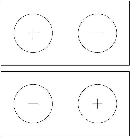
Figure 1. If all the energy ends up in the lowest wavenumber mode of the rectangular domain, it must occupy one of the two states depicted.

Equilibrium statistical mechanics [4] predicts the statistically steady state attained by this system after an undetermined period of adjustment. Interest attaches to the sequence of equilibrium states that occur as $k_c\to \infty$. In this limit, the theory predicts that all of the energy ends up in the lowest-wavenumber mode, and that all of the enstrophy not contained in that mode appears in modes near $k_c$. As $k_c\to \infty$, this excess enstrophy is expelled to infinity, disappearing in much the same way as if it had been removed by viscosity. The tendency for all the energy to crowd into a single lowest mode is often referred to as ‘Bose–Einstein condensation’, after a closely analogous result in quantum mechanics.

Suppose that the initial conditions are such that the conserved circulation around the rectangular boundary vanishes. Then the lowest-wavenumber mode, which has a single extremum within the rectangle, remains unexcited. All of the energy flows into the next-lowest mode, the one depicted in Figure 1. Because the boundary is a rectangle (and not, say, a square or a circle), there is only one next-lowest mode. If all of the energy ends up in this mode, it must appear in one of the two states depicted in Figure 1. Moreover, once either of these states is established, the system cannot flip suddenly to the opposite state because that would require the energy in one of these states to flow temporarily into higher-wavenumber modes, and that, according to statistical mechanics, is extremely unlikely. Thus, the two states depicted in Figure 1 act as a single-register binary memory. The state that actually occurs is an accident of the initial conditions, but once established, it lasts for a very long time. If the conserved circulation around the perimeter of the rectangle does not vanish, the amplitude of the lowest mode remains fixed at a nonzero value, but the Bose–Einstein condensation would still proceed only as far as the next-lowest mode depicted in Figure 1.

Still considering flow on the plane, suppose that there are two lowest modes available to receive all the energy. For the statistical mechanics, we take the microcanonical ensemble as seems appropriate. Let the energy be $E=x^2+y^2$, where x and y are the amplitudes of the two modes. If x is the only mode, then, as already noted, its probability distribution would be

$$P(x)=\delta (x-\sqrt{E})+\delta (x+\sqrt{E})$$

(1)

where $\delta (·)$ is Dirac’s delta function and, here and below, we ignore normalization constants. However, if there are two modes, then the probability distribution of either mode is

$$P(x)={\int }_{-\infty }^{+\infty }dy\delta (x^2+y^2-E)\propto \frac{1}{\sqrt{E-x^2}}$$

(2)

if $x^2<E$ and zero otherwise. Like (1), the distribution (2) is sharply peaked at $\pm \sqrt{E}$, but now there is significant probability of finding x anywhere in between. If there are three lowest modes, then the analogous calculation predicts that x is uniformly distributed between $\pm \sqrt{E}$. The implication of these calculations is clear: if the lowest available mode is degenerate with two or more members, then each member sees the other members as a reservoir from which energy may be borrowed or loaned, allowing leakage between states and a breakdown of memory. In all of these examples, the average flow predicted by statistical mechanics is misleading and beside the point. For example, if the ensemble consists of the two equal-probability states depicted in Figure 1, then the average flow vanishes, but a vanishing velocity field is very unrepresentative of either state. Such considerations demonstrate how even the simplest calculations with probability distributions require careful interpretation.

Now consider the corresponding equilibrium state on the sphere [5]. Spherical harmonics replace Fourier modes, and the harmonic degree n with cutoff $n_c$ replaces the wavenumber k with cutoff $k_c$. The lowest mode $Y_0^0$ is irrelevant because the stream function is arbitrary by a constant and because the vorticity integrates to zero over the sphere (Gauss’s constraint). The next lowest modes are three: $Y_1^0$, $Y_1^{\pm 1}$. However, the amplitudes of these three modes are determined by the three components of angular momentum, which is conserved by our dynamics, even with nonzero viscosity. Thus, the lowest-degree modes into which the energy can pile up are those of degree $n=2$, namely, $Y_2^0$, $Y_2^{\pm 1}$, $Y_2^{\pm 2}$. By the reasoning of the previous paragraph, the Bose–Einstein condensate would be one in which these five modes freely exchange energy. Instead, it turns out, the five modes of degree two lock together in a pattern that is perfectly static in a uniformly rotating reference frame. This behavior is dramatically different from flow on the plane, and is solely a consequence of spherical geometry.

Let the sphere be centered at $x=y=z=0$, and suppose, without loss of generality, that the angular momentum (if nonzero) points toward positive z. Then, the amplitude of the $Y_1^0$-mode is a nonzero constant, and the amplitudes of $Y_1^{\pm 1}$ vanish. The $Y_1^0$-mode corresponds to a solid-body flow about the z-axis with constant angular speed $\Omega$, and the corresponding vorticity is called the Coriolis parameter. As shown in Section 3, the flow consisting of the $Y_1^0$-mode and the 5 $Y_2$-modes with arbitrary amplitudes represents an exact solution to the inviscid vorticity equation on the sphere. If $\Omega =0$, this flow field is steady in the inertial frame. If $\Omega \ne 0$, the flow field is steady in a reference frame rotating at speed $2\Omega /3$ with respect to the inertial frame. The amplitude $\Omega$ of the $Y_1^0$-mode is determined by the conserved angular momentum. The amplitudes of the $Y_2$-modes are accidents of the initial conditions in the same way that the initial conditions determine which of the two states in Figure 1 eventually emerge. However, once these amplitudes are determined via Bose–Einstein condensation, they persist indefinitely under the stated assumptions. Thus, Bose–Einstein condensation into $Y_2$-modes represents a potential memory storage that does not, as in planar geometry, require a ‘probability well’ for its preservation. For the plane, as for the sphere, triads with the same wavenumber magnitude (the analog of spherical harmonic degree) do not interact, either with each other or with modes of different wavenumber magnitude. However, typical planar geometries forbid the occurrence of many modes with the same wavenumber magnitude. For instance, in the case of an infinitely periodic box, in which the wave vector corresponds to integer pairs $(n,m)$, modes with the same $n^2+m^2$ are rare. We come back to this in Section 6.

More generally, flow consisting only of $Y_1$ modes and modes of a single spherical harmonic degree n is perfectly static in a reference frame rotating at angular speed

$$\Omega -\frac{2\Omega }{n(n+1)}$$

(3)

with respect to the inertial frame. According to [6], this result was known to Ertel. Section 3 supplies details. There are $2n+1$ spherical harmonics with the same degree n. These facts invite us to think of the stream function for flow on the sphere as the sum

$$\psi (\xi ,\eta ,t)=\sum _{n=1}^{\infty }{\psi }_n(\xi ,\eta ,t)$$

(4)

of contributions ${\psi }_n$ of degree n, where each ${\psi }_n$ is itself the sum of $2n+1$ spherical harmonics. The coordinates $(\xi ,\eta )$ are arbitrary, but we strongly prefer them to be stereographic coordinates. Again, if only ${\psi }_1$ and one ${\psi }_n$ with $n>1$ are present, then $\psi$ is steady in the frame rotating at angular speed (3). In the general case where all ${\psi }_n$ are present, the various ${\psi }_n$ interact to produce a turbulent flow. However, the interaction between ${\psi }_n$ with very different autorotation rates (3)—very different n—is likely to be weak. Additionally, since the difference between autorotation rates is greatest and varies most rapidly at small n, we expect the energy transfer to large spatial scales to slow dramatically as the energy reaches low n for sufficiently large $\Omega$. This is essentially Rhines’s ‘beta-arrest’ phenomenon for flow on the beta plane [7] but now taking a form particular to the sphere. See also [8].

This study was begun with the hope that the special static solutions described above might be a factor in intermediate-range weather prediction. Although flickers of that hope remain, there are significant differences between the Earth’s atmosphere and the very idealized dynamics considered in this paper. First and foremost, angular momentum conservation applies only to the entire Earth–atmosphere–ocean system. Mountain torque provides the main coupling between the atmosphere and the solid planet. The latter, with its enormously greater moment of inertia, experiences only small changes in its rotation rate, but fluctuations in the $Y_1^0$ component of atmospheric flow are very significant and lead to a peak in the atmospheric energy spectrum at $n=1$ [9]. Second, because the Rhines scale corresponding to the Earth’s atmosphere is smaller than the planetary radius, beta-arrest prevents the leftward movement of energy through the spectrum from reaching $n=2$. As a result of these two factors, the atmospheric energy spectrum actually shows a minimum at $n=2$. See [10] for the statistical mechanics including mountain torque and [11] for a thorough review of the atmospheric angular momentum.

The plan of the paper is as follows. In Section 2 and Appendix A, we derive the Navier–Stokes equations for flow on the sphere in stereographic coordinates. The form of the viscosity for flow on curved surfaces has been the subject of disagreement. For instance, the viscosity given by [12] does not conserve angular momentum. We follow the recommendation of [13] that the viscosity conserves angular momentum, and in Appendix A, we show that their recommended viscosity takes an especially simple form in stereographic coordinates.

In Section 3, we prove the special solutions described briefly above. Our proof using stereographic coordinates is substantially simpler than the proofs given by [14] or [15] using spherical coordinates.

In Section 4 and Appendix B, we use the method of [16] to construct an Arakawa-type model in stereographic coordinates. The model conserves energy and enstrophy when the viscosity vanishes.

Section 5 demonstrates the accuracy of the model and tests our speculation that Bose–Einstein condensation on the sphere produces a static flow. Our results suggest that the time required to achieve the static state is probably infinite but that the flow rather quickly becomes quasi-static.

It is a pleasure to dedicate this paper to the memory of Jack Herring. Rick Salmon acknowledges the importance of Jack’s mentorship at an early stage of his career and holds the happy memories of a lifelong friendship. Rick cannot think of Jack without also remembering his wife Betty, who shared Jack’s kind and generous spirit, and greatly enjoyed the foibles and eccentricities of his scientific friends.

2. Stereographic Coordinates

We solve the vorticity equation for incompressible flow on the unit sphere,

$$x^2+y^2+z^2=1.$$

(5)

We refer to the point $(x,y,z)=(0,0,1)$ as the ‘north pole’, and $(x,y,z)=(0,0,-1)$ as the ‘south pole’, even when the angular momentum vanishes, the case commonly referred to as ‘non-rotating’. The ‘equator’ is the intersection of the plane $z=0$ with (5). The conserved angular momentum is a vector in the direction of $(0,0,1)$.

Besides the Cartesian embedding coordinates $(x,y,z)$, we shall refer to three other coordinate systems. The first of these are the usual spherical coordinates, defined by

$$\begin{array}{cc}\hfill x& =cos\theta cos\lambda \hfill \\ \hfill y& =cos\theta sin\lambda \hfill \\ \hfill z& =sin\theta \hfill \end{array}$$

(6)

where $\lambda$ is the longitude and $\theta$ the latitude. The $(\lambda ,\theta )$ coordinates cover the sphere, except for singularities at the two poles. We also use the stereographic coordinates

$$\xi =\frac{x}{1-z},\eta =\frac{y}{1-z}$$

(7)

defined by a line, emanating from the north pole, that intersects the equatorial plane at $(\xi ,\eta ,0)$ and the sphere at $(x,y,z)$. $(\xi ,\eta )$ cover the sphere except for a singularity at infinity, corresponding to the north pole. We also use

$$\widehat{\xi }=\frac{x}{1+z},\widehat{\eta }=\frac{y}{1+z}$$

(8)

defined by the intersection with the equatorial plane of a line emanating from the south pole. $(\widehat{\xi },\widehat{\eta })$ cover the sphere, except for singularity at infinity corresponding to the south pole. The stereographic systems (7) and (8) prove to be more useful than the spherical coordinates; the primary challenge is to match them together. Our strategy is to solve the southern hemisphere dynamics in $(\xi ,\eta )$ within the unit circle

$${\xi }^2+{\eta }^2<1,$$

(9)

to solve the northern hemisphere dynamics in $(\widehat{\xi },\widehat{\eta })$ within the unit circle

$${\widehat{\xi }}^2+{\widehat{\eta }}^2<1,$$

(10)

and to match the two solutions together at the equator,

$${\xi }^2+{\eta }^2={\widehat{\xi }}^2+{\widehat{\eta }}^2=1.$$

(11)

The transformation equations between the two stereographic systems are

$$(\xi ,\eta )=\frac{1}{{\widehat{r}}^2}(\widehat{\xi },\widehat{\eta }),(\widehat{\xi },\widehat{\eta })=\frac{1}{r^2}(\xi ,\eta )$$

(12)

where

$$r^2\equiv {\xi }^2+{\eta }^2,{\widehat{r}}^2\equiv {(\widehat{\xi })}^2+{(\widehat{\eta })}^2.$$

(13)

A useful relation is

$$r\widehat{r}=1.$$

(14)

Points within the unit circle on the $(\widehat{\xi },\widehat{\eta })$ plane transform to points outside the unit circle on the $(\xi ,\eta )$ plane, and vice versa. On the equator itself, $(\xi ,\eta )=(\widehat{\xi },\widehat{\eta })$. It is also useful to record the inverse transformations from either set of stereographic coordinates to the Cartesian embedding coordinates,

$$\begin{array}{cc}\hfill x& =\frac{2\xi }{{\xi }^2+{\eta }^2+1}=\frac{2\widehat{\xi }}{{\widehat{\xi }}^2+{\widehat{\eta }}^2+1}\hfill \end{array}$$

(15)

$$\begin{array}{cc}\hfill y& =\frac{2\eta }{{\xi }^2+{\eta }^2+1}=\frac{2\widehat{\eta }}{{\widehat{\xi }}^2+{\widehat{\eta }}^2+1}\hfill \end{array}$$

(16)

$$\begin{array}{cc}\hfill z& =\frac{{\xi }^2+{\eta }^2-1}{{\xi }^2+{\eta }^2+1}=\frac{1-{\widehat{\xi }}^2-{\widehat{\eta }}^2}{{\widehat{\xi }}^2+{\widehat{\eta }}^2+1}.\hfill \end{array}$$

(17)

For a thorough introduction to stereographhic coordinates, see [17,18].

Infinitesimal displacements on the surface of the sphere satisfy

$$\begin{array}{cc}\hfill d{s}^2=d{x}^2+d{y}^2+d{z}^2& ={cos}^2\theta d{\lambda }^2+d{\theta }^2\hfill \\ \hfill & =\frac{4}{{\left(1+{\xi }^2+{\eta }^2\right)}^2}\left(d{\xi }^2+d{\eta }^2\right)\hfill \\ \hfill & =\frac{4}{{\left(1+{\widehat{\xi }}^2+{\widehat{\eta }}^2\right)}^2}\left(d{\widehat{\xi }}^2+d{\widehat{\eta }}^2\right)\hfill \end{array}$$

(18)

where $ds$ is the infinitesimal distance tangent to the surface of the sphere. Thus, all of our systems fit the general form

$$d{s}^2=h_1{({\xi }_1,{\xi }_2)}^2{(d{\xi }_1)}^2+h_2{({\xi }_1,{\xi }_2)}^2{(d{\xi }_2)}^2$$

(19)

where $({\xi }_1,{\xi }_2)$ are general orthogonal coordinates, and $\mathrm{diag}(h_1^2,h_2^2)$ is the metric tensor. In arbitrary orthogonal coordinates, the incompressibility condition takes the form

$$\frac{\partial }{\partial {\xi }_1}\left(h_1{h}_2{\dot{\xi }}_1\right)+\frac{\partial }{\partial {\xi }_2}\left(h_1{h}_2{\dot{\xi }}_2\right)=0$$

(20)

where the overdot denotes the time derivative following a fluid particle. Since the velocity components tangent to the sphere in the directions of ${\xi }_1$ and ${\xi }_2$ are, respectively,

$$U_1=h_1{\dot{\xi }}_1,U_2=h_2{\dot{\xi }}_2$$

(21)

(20) is equivalent to

$$\frac{\partial }{\partial {\xi }_1}\left(h_2{U}_1\right)+\frac{\partial }{\partial {\xi }_2}\left(h_1{U}_2\right)=0$$

(22)

which implies

$$U_1=-\frac{1}{h_2}\frac{\partial \psi }{\partial {\xi }^2},U_2=+\frac{1}{h_1}\frac{\partial \psi }{\partial {\xi }^1}$$

(23)

where $\psi ({\xi }_1,{\xi }_2,t)$ is the stream function. The vorticity equation takes the form

$$q_t+\frac{1}{h_1{h}_2}\frac{\partial (\psi ,q)}{\partial ({\xi }_1,{\xi }_2)}=0$$

(24)

where

$$q={\nabla }_{LB}^2\psi$$

(25)

is the vorticity, and

$${\nabla }_{LB}^2\psi \equiv \frac{1}{h_1{h}_2}\left(\frac{\partial }{\partial {\xi }_1}\left(\frac{h_2}{h_1}\frac{\partial \psi }{\partial {\xi }_1}\right)+\frac{\partial }{\partial {\xi }_2}\left(\frac{h_1}{h_2}\frac{\partial \psi }{\partial {\xi }_2}\right)\right)$$

(26)

is the Laplace–Beltrami operator.

In the case of spherical coordinates, $({\xi }_1,{\xi }_2)=(\lambda ,\theta )$, $(h_1,h_2)=(cos\theta ,1)$, and (23)–(25) take the familiar forms

$$U_{\lambda }=-\frac{\partial \psi }{\partial \theta },U_{\theta }=+\frac{1}{cos\theta }\frac{\partial \psi }{\partial \lambda }$$

(27)

$$q_t+\frac{1}{cos\theta }\frac{\partial (\psi ,q)}{\partial (\lambda ,\theta )}=0$$

(28)

and

$$q=\frac{1}{{cos}^2\theta }\frac{{\partial }^2\psi }{\partial {\lambda }^2}+\frac{1}{cos\theta }\frac{\partial }{\partial \theta }\left(cos\theta \frac{\partial \psi }{\partial \theta }\right)\equiv {\nabla }_{LB}^2\psi .$$

(29)

To obtain the dynamics in stereographic coordinates, we proceed from the general Equations (24) and (25). Some care must be taken concerning the handedness of the coordinate systems. Viewed from the exterior of the unit sphere, $(\widehat{\xi },\widehat{\eta })$ and $(\lambda ,\theta )$ constitute right-handed systems, whereas $(\xi ,\eta )$ constitutes a left-handed system. That is,

$$\frac{\partial (\widehat{\xi },\widehat{\eta })}{\partial (\lambda ,\theta )}>0,\frac{\partial (\xi ,\eta )}{\partial (\lambda ,\theta )}<0.$$

(30)

The general covariant point of view cares nothing about handedness, but we want our computed vorticity and stream function to be the same as would be obtained by solving the entire problem in spherical coordinates, and, in particular, we want these quantities to be continuous at the equator; it would be a great nuisance to keep track of differently defined stream functions in the two hemispheres. With this in mind, the northern hemisphere equations take the forms

$${\widehat{h}}^2{q}_t+\frac{\partial (\psi ,q)}{\partial (\widehat{\xi },\widehat{\eta })}=0,{\widehat{h}}^{2}q={\widehat{\nabla }}^2\psi ,\widehat{h}=\frac{2}{1+{\widehat{\xi }}^2+{\widehat{\eta }}^2}$$

(31)

within the unit circle (10); the southern hemisphere equations take the forms

$$h^2{q}_t-\frac{\partial (\psi ,q)}{\partial (\xi ,\eta )}=0,h^{2}q={\nabla }^2\psi ,h=\frac{2}{1+{\xi }^2+{\eta }^2}$$

(32)

within the unit circle (9). Here,

$${\nabla }^2\psi \equiv \frac{{\partial }^2\psi }{\partial {\xi }^2}+\frac{{\partial }^2\psi }{\partial {\eta }^2},{\widehat{\nabla }}^2\psi \equiv \frac{{\partial }^2\psi }{\partial {\widehat{\xi }}^2}+\frac{{\partial }^2\psi }{\partial {\widehat{\eta }}^2}.$$

(33)

The Laplace–Beltrami operator in (26) and (29) is equivalent to ${\widehat{h}}^{-2}{\widehat{\nabla }}^2$ and $h^{-2}{\nabla }^2$. Apart from the factors of h and $\widehat{h}$, (31)–(33) have the same form as the corresponding equations for planar geometry in Cartesian coordinates. This greatly facilitates numerical solution. The sign change between (31) and (32) reflects the change in handedness. To see that this makes sense, recall that the first equation in (31) and (32) also applies to a passive scalar advected by the velocity field represented by $\psi$. The sign change between (31) and (32) ensures that the (cross-equatorial) flux of q out of the unit circle (9) matches the flux of q into the unit circle (10), with no need to redefine or re-interpret $\psi$ or q.

Alternatively, by replacing the vorticity q in (31) and (32) by

$$q+f\equiv q+2\Omega sin\theta =q+2\Omega z=q+2\Omega \frac{{\xi }^2+{\eta }^2-1}{{\xi }^2+{\eta }^2+1}=q+2\Omega \frac{1-{\widehat{\xi }}^2-{\widehat{\eta }}^2}{{\widehat{\xi }}^2+{\widehat{\eta }}^2+1}$$

(34)

we obtain the equations of motion in a frame rotating at angular speed $\Omega$.

We solve (31) on (10), and (32) on (9), with the matching conditions that $\psi$ and q are continuous at the equator (11). If the initial condition is given by prescribing q, then q must satisfy the Gauss constraint,

$$\int \int d\xi d\eta h^{2}q+\int \int d\widehat{\xi }d\widehat{\eta }{\widehat{h}}^{2}q=0$$

(35)

where the integrals are over the two unit circles (i.e., the whole sphere), but the constraint (35) is automatically maintained thereafter. If the initial condition is given by prescribing $\psi$, the Gauss constraint is automatically satisfied.

Although we work primarily with (31) and (32), it is useful to record the corresponding forms of the momentum equations. Introducing the notation,

$$(u,v)\equiv h^2(\dot{\xi },\dot{\eta })$$

(36)

the southern hemisphere equations take the forms

$$\begin{array}{cc}\hfill \frac{\partial u}{\partial t}-qv& =-\frac{\partial p}{\partial \xi }\hfill \end{array}$$

(37)

$$\begin{array}{cc}\hfill \frac{\partial v}{\partial t}+qu& =-\frac{\partial p}{\partial \eta }\hfill \end{array}$$

(38)

$$\begin{array}{cc}\hfill \frac{\partial u}{\partial \xi }+\frac{\partial v}{\partial \eta }& =0\hfill \end{array}$$

(39)

$$\begin{array}{cc}\hfill q& =\frac{1}{h^2}\left(\frac{\partial v}{\partial \xi }-\frac{\partial u}{\partial \eta }\right).\hfill \end{array}$$

(40)

The northern hemisphere equations take the same form as (37)–(40) but with hats applied to all the variables except q. Again, if $h^2=1$, (37)–(40) are formally identical to the equations for two-dimensional incompressible motion in planar geometry. However, no choice of variables can make $h^2$ equal unity on the unit sphere; instead it must obey the requirement

$$\frac{1}{h^4}\left[\frac{\partial h}{\partial {\xi }_1}\frac{\partial h}{\partial {\xi }_1}+\frac{\partial h}{\partial {\xi }_2}\frac{\partial h}{\partial {\xi }_2}-h\left(\frac{{\partial }^{2}h}{\partial {\xi }_1^2}+\frac{{\partial }^{2}h}{\partial {\xi }_2^2}\right)\right]=1$$

(41)

that the Gaussian curvature be uniform and equal to unity. The effects of curvature can never be transformed away, but it is interesting that they can be confined to a single factor in (40). This is what motivates the definition (36). However, it must be emphasized that the symbols $(u,v)$ invite misinterpretation: the velocity of fluid particles tangent to the sphere is

$$(U,V)=h(\dot{\xi },\dot{\eta })=\frac{1}{h}(u,v)$$

(42)

and not $(u,v)$.

The inviscid dynamics (31) and (32) or (37)–(40) conserve energy in the form,

$$E=\frac{1}{2}\int \int d\xi d\eta \nabla \psi ·\nabla \psi$$

(43)

where $\nabla \psi \equiv (\partial \psi /\partial \xi ,\partial \psi /\partial \eta )$, total vorticity in the form

$$\int \int d\xi d\eta h^{2}q=\int \int d\xi d\eta {\nabla }^2\psi \equiv 0$$

(44)

and enstrophy in the form

$$Z=\frac{1}{2}\int \int d\xi d\eta h^2{q}^2=\frac{1}{2}\int \int d\xi d\eta h^{-2}{({\nabla }^2\psi )}^2.$$

(45)

The integrations in (43)–(45) are over the whole sphere, with the understanding that they are actually computed as the sum of integrations over the two unit circles. The vanishing of (44) corresponds to the Gauss constraint. More generally, the inviscid dynamics conserves Casimirs of the form

$$\int \int d\xi d\eta h^{2}F(q)$$

(46)

where $F(q)$ is any function of the vorticity, for which the integral in (46) converges; (44) and (45) are particularly important cases of (46).

The inviscid dynamics also conserves angular momentum. Angular momentum is a vector with three components, each of which is conserved. However, since the location of the axis that determines the origin of our stereographic system has no particular significance, we may assume, without loss of generality, that the angular momentum vector points in the z-direction. Then, the sole nonvanishing component of angular momentum is

$$M=\int \int d\xi d\eta h^2(\xi v-\eta u)=\int \int d\xi d\eta h^{3}q=\int \int d\xi d\eta h{\nabla }^2\psi .$$

(47)

It remains to discuss the viscosity. In [13], Gilbert et al. examine three proposed definitions of viscosity for incompressible flow on a curved surface. All three are covariant, and none of the three can be rejected on purely fundamental grounds. However, only one of the three forms of viscosity conserves angular momentum. We agree with [13] that the angular-momentum-conserving form is the proper choice for applications in which the viscosity is actually an eddy viscosity representing the mixing—but not the destruction—of angular momentum by unresolved motions. In Appendix A, we show that the viscosity suggested by [13] takes the surprisingly simple form

$$\begin{array}{cc}\hfill \frac{\partial u}{\partial t}+\cdots & =-\nu \frac{\partial q}{\partial \eta }\hfill \end{array}$$

(48)

$$\begin{array}{cc}\hfill \frac{\partial v}{\partial t}+\cdots & =+\nu \frac{\partial q}{\partial \xi }\hfill \end{array}$$

(49)

in the dynamics (37)–(40), and

$${\widehat{h}}^2{q}_t+\cdots =\nu {\widehat{\nabla }}^{2}q,h^2{q}_t+\cdots =\nu {\nabla }^{2}q$$

(50)

in the dynamics (31) and (32). The ellipses represent the conservative terms already discussed. When the viscosity in (50) is added to the dynamics (31) and (32), we find that

$$\frac{dE}{dt}=-\nu \int \int d\xi d\eta h^2{q}^2$$

(51)

$$\frac{dZ}{dt}=-\nu \int \int d\xi d\eta \nabla q·\nabla q$$

(52)

and

$$\frac{dM}{dt}=0.$$

(53)

Thus, viscosity dissipates energy and enstrophy, but not angular momentum. The importance of angular momentum conservation by viscosity seems not to be widely appreciated, but see [19] and references therein.

Many modelers prefer a more scale-selective hyperviscosity to any form of Navier–Stokes viscosity. However, hyperviscosity introduces non-physical effects. For example, hyperviscosity creates artificial local extrema in vorticity [20]. For this reason, we believe that Navier–Stokes viscosity is well worth the extra cost in spatial resolution.

We emphasize that, in our dynamics, the sphere plays no role except to shape the flow. Without drag or mountain torque, only curvature and angular momentum conservation distinguish our dynamics from the flow in a box on the plane.

3. Exact Solutions

Let $Y_n$ be any solution of

$${\nabla }_{LB}^2{Y}_n=-n(n+1)Y_n$$

(54)

where n is a positive integer. The coordinate system used to represent $Y_n$ is arbitrary. In a spherical coordinate system, the general solution of (54) is

$$Y_n(\theta ,\lambda )=\sum _{m=0}^n{A}_m{P}_n^m(sin\theta )cos\left(m\lambda +{\gamma }_m\right)$$

(55)

where $P_n^m$ is a Legendre function of the first kind, and $A_m$ and ${\gamma }_m$ are arbitrary constants. We recognize (55) as the sum of all spherical harmonics of degree n with arbitrary amplitudes $A_m$ and phases ${\gamma }_m$. The customary normalization coefficients have been lumped into the $A_m$. The representation (55) applies to any system of spherical coordinates. That is, if we transform (55) to an alternative set of spherical coordinates—obtained, for example, by changing the polar axis with respect to which the spherical harmonics are defined—we obtain an expression identical to (55) but with a different set of $A_m$’s and ${\gamma }_m$’s. We may in fact use any system of coordinates, including the more convenient stereographic coordinates, because the following proof relies only on the covariant property (54).

Let ${\psi }_{(l,m,n)}^{\Omega }$ be the streamfunction corresponding to solid-body flow at angular speed $\Omega$ about an axis in the direction of the unit vector $(l,m,n)$. Let $Y_n$ be a solution of (54), and let $Y_n^{\omega }$ be the pattern $Y_n$ rotating at the angular speed

$$\omega =\Omega -\frac{2\Omega }{n(n+1)}$$

(56)

about the axis $(l,m,n)$. Then

$$\psi ={\psi }_{(l,m,n)}^{\Omega }+Y_n^{\omega }$$

(57)

is a solution of our dynamics. For example, if $(l,m,n)=(0,0,1)$, and if the spherical harmonics are defined with respect to this same axis, then the solution (57) takes the form

$$\psi (\theta ,\lambda ,t)=-\Omega sin\theta +\sum _{m=1}^n{A}_m{P}_n^m(sin\theta )cos\left(m(\lambda -\omega t)+{\gamma }_m\right)$$

(58)

in spherical coordinates. However, the axis $(l,m,n)$ is arbitrary, and, more importantly, the spherical harmonics can be defined with respect to any axis whatsoever; it only matters that they are all of degree n. In fact, the solution (57), properly interpreted, holds in any system of coordinates. Viewed from a reference frame rotating with the solid-body flow—that is, viewed in rotating coordinates—the solution (57) corresponds to a retrograde, ‘pseudo-westward’, propagation of the $Y_n$-pattern at an angular velocity equal to the last term in (56), which differs from the frequency of Rossby–Haurwitz waves in its lack of a factor m in the numerator. This m factor is missing because we here define $\omega$ as angular frequency rather than wave frequency. That is, in (58) we write $m(\lambda -\omega t)$ rather than $m\lambda -\omega t$.

In [6] Kochin et al. attribute the solution (57) to Hans Ertel in 1945, but they do not give a reference. See also [21]. It was re-discovered by Herring’s colleague Phil Thompson [14] for the special case in which $(l,m,n)$ coincides with the z-axis, as in (58), and $Y_n$ consists of a single spherical harmonic whose axis of symmetry is inclined with respect to the z-axis by a prescribed angle. Thompson proposed this special exact solution as a test of numerical codes based on spherical coordinates. In [15], Verkley matched Thompson’s solution in one region of the sphere with an analogous solution in another region in which $Y_n$ is replaced by the solutions of ${\nabla }_{LB}^2{Y}_n=d{Y}_n$, with d a positive constant. The matching conditions are that the two solutions precess about the z-axis at the same angular speed and have continuous derivatives at the boundary between regions. The family of solutions discovered by Ertel, Thompson, and Verkley is noteworthy in that they seem to be the only analytic solutions of the vorticity equation on the sphere (besides ‘zonal’ flows in which $\psi =F(\theta )$ with F arbitrary) that do not include point vortices. See also [22] and the references therein.

We prove (57) using stereographic coordinates. Because rotations are involved, it is best to use the complex notation $\zeta =\xi +i\eta$ and to regard $\psi (\xi ,\eta ,t)$, $q(\xi ,\eta ,t)$ as $\psi (\zeta ,\overline{\zeta },t)$, $q(\zeta ,\overline{\zeta },t)$, where $\overline{\zeta }=\xi -i\eta$ denotes the complex conjugate. In this notation,

$${\nabla }_{LB}^2={(1+\zeta \overline{\zeta })}^2\frac{{\partial }^2}{\partial \zeta \partial \overline{\zeta }}$$

(59)

and the dynamics (32) takes the form

$$h^2{q}_t+2i\frac{\partial (\psi ,q)}{\partial (\zeta ,\overline{\zeta })}=0,q={\nabla }_{LB}^2\psi ,h=\frac{2}{1+\zeta \overline{\zeta }}$$

(60)

given by [23]. Suppose, without loss of generality, that the axis of the solid body flow is $(0,0,1)$. Then

$${\psi }_{(0,0,1)}^{\Omega }=-\Omega sin\theta =-\Omega z=-\Omega \frac{({\xi }^2+{\eta }^2-1)}{({\xi }^2+{\eta }^2+1)}=-\Omega \frac{(\zeta \overline{\zeta }-1)}{(\zeta \overline{\zeta }+1)}=\Omega h-\Omega .$$

(61)

The last term in (61) is an irrelevant constant. Let $Y_n(\zeta ,\overline{\zeta })$ be a solution of (54). To demonstrate Thompson’s solution, we must show that

$$\psi =Y_n(s,\overline{s})+\Omega h$$

(62)

satisfies (60), where

$$s\equiv \zeta e^{-i\omega t},\overline{s}\equiv \overline{\zeta }{e}^{+i\omega t}$$

(63)

and $\omega$ is given by (56). In the new coordinates $s,\overline{s}$,

$${\nabla }_{LB}^2={(1+s\overline{s})}^2\frac{{\partial }^2}{\partial s\partial \overline{s}},h=\frac{2}{1+s\overline{s}}.$$

(64)

The vorticity corresponding to (62) is

$$q={\nabla }_{LB}^2\left(Y_n(s,\overline{s})+\Omega h\right)=-n(n+1)Y_n(s,\overline{s})-2\Omega h+2\Omega .$$

(65)

The last term in (65) is needed to satisfy the Gauss constraint, but it does not contribute to the vorticity equation, in which only derivatives of q appear. By the chain rule,

$$\begin{array}{cc}\hfill h^2{q}_t=-n(n+1)h^2\frac{\partial }{\partial t}{Y}_n(s,\overline{s})& =-n(n+1)i\omega h^2\left(-s\frac{\partial Y_n}{\partial s}+\overline{s}\frac{\partial Y_n}{\partial \overline{s}}\right)\hfill \\ \hfill & =-2n(n+1)i\omega \frac{\partial (Y_n,h)}{\partial (s,\overline{s})}\hfill \end{array}$$

(66)

where we used the identities

$$\frac{\partial h}{\partial s}=-\frac{1}{2}{h}^2\overline{s},\frac{\partial h}{\partial \overline{s}}=-\frac{1}{2}{h}^{2}s.$$

(67)

For the second term in the vorticity equation, we have

$$2i\frac{\partial (\psi ,q)}{\partial (\zeta ,\overline{\zeta })}=2i\frac{\partial (Y_n+\Omega h,-n(n+1)Y_n-2\Omega h)}{\partial (s,\overline{s})}=2\Omega i\left(n(n+1)-2\right)\frac{\partial (Y_n,h)}{\partial (s,\overline{s})}.$$

(68)

The sum of (66) and (68) vanishes for $\omega$ given by (56). Thus, (62) satisfies our dynamics for any positive integer n. This proof is simpler than the proofs given by [14] or [15] using spherical coordinates.

4. Numerical Model

We solve (31) and (32) by the method of [16], a generalization of Arakawa’s method [24] that conserves discrete analogues of the energy (43), total vorticity (44), and enstrophy (45) when $\nu =0$. This method was further generalized to the shallow water equations; see [25] and references therein.

We begin by noting that the vorticity equation in (32) is equivalent to the statement that

$$\int \int d\xi d\eta \alpha h^2{q}_t=\int \int d\xi d\eta \alpha \frac{\partial (\psi ,q)}{\partial (\xi ,\eta )}$$

(69)

for any function $\alpha (\xi ,\eta )$. The integration is over the entire sphere. By parts integrations, (69) takes the more useful form

$$\int \int d\xi d\eta \alpha h^2{q}_t=\frac{1}{3}\int \int d\xi d\eta \left[\alpha \frac{\partial (\psi ,q)}{\partial (\xi ,\eta )}+\psi \frac{\partial (q,\alpha )}{\partial (\xi ,\eta )}+q\frac{\partial (\alpha ,\psi )}{\partial (\xi ,\eta )}\right].$$

(70)

Our strategy is to discretize all the variables in (70) in such a way that the conservation of energy, total vorticity, and enstrophy correspond to purely algebraic cancellations between the terms. The conservation of enstrophy (45) corresponds to the choice $\alpha =q$ in (70). This requires that the discrete form of

$$\int \int d\xi d\eta \left[q\frac{\partial (\psi ,q)}{\partial (\xi ,\eta )}+\psi \frac{\partial (q,q)}{\partial (\xi ,\eta )}+q\frac{\partial (q,\psi )}{\partial (\xi ,\eta )}\right]$$

(71)

vanishes, and this occurs automatically if the discrete Jacobian is antisymmetric. The conservation of total vorticity corresponds to $\alpha =1$, and requires that the discrete form of

$$\int \int d\xi d\eta \frac{\partial (\psi ,q)}{\partial (\xi ,\eta )}$$

(72)

vanishes. Again, this occurs automatically. Energy conservation corresponds to $\alpha =-\psi$, and we discuss it further below.

We discretize (70) by covering the interior of both stereographic circles with quadrilateral finite elements. The placement of the elements is the same in both circles. Most of the elements are perfect squares, as illustrated in Figure 2 for a very low-resolution case, but near the unit circle itself, the quadrilaterals are deformed, with one or more nodes lying on the circle.

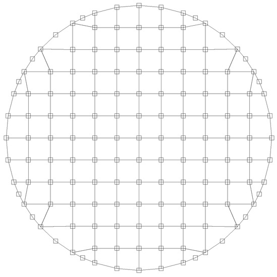
Figure 2. Quadrilateral elements cover the interior of the unit circle in the stereographic plane. The circle itself corresponds to the equator. Most of the interior elements are perfect squares. Elements with 1, 2, or 3 equatorial nodes are deformed quadrilaterals that conform to the circle.

The nodal values of $\psi$ and q are the dependent variables of the model. Each interior node corresponds to a point on one of the hemispheres, and is shared by four elements. Each equatorial node is shared by up to six elements, counting elements on both sides of the equator. At every time, the state of the system is determined by the values of $\psi$ or q at $N=2N_i+N_{eq}$ nodes, where $N_i$ is the number of interior nodes within each of the two unit circles, and $N_{eq}$ is the number of (shared) equatorial nodes. Appendix B offers further details.

In claiming conservation properties, we regard time derivatives as exact. That is, we ignore errors that result from the finite time step. Experience shows these errors to be small in comparison to those that result from space discretization. This issue arises when we consider the finite-element discretization of the left-hand side of (70), namely

$$\sum _i{A}_i{\alpha }_i{h}_i^2\frac{d{q}_i}{dt}$$

(73)

where the summation is over all N nodes, $A_i$ is the area of the $\xi \eta$-plane associated with node i (in a sense to be made precise), and ${\alpha }_i$, $h_i$, $q_i$ are the nodal values of $\alpha$, q and h. Note that the metric factor

$$h_i=\frac{2}{1+{\xi }_i^2+{\eta }_i^2}$$

(74)

is determined by the arrangement of the quadrilateral elements, and is independent of time. Replacing the left-hand side of (70) with (73) and the right-hand side of (70) with the finite-element representation described briefly above and more thoroughly in Appendix B, we obtain the model dynamics by requiring that the discrete form of (70) vanishes for arbitrary nodal values ${\alpha }_i$. Setting ${\alpha }_i=q_i$ and treating the time derivative as exact, we conclude that the discrete enstrophy

$$Z\equiv \frac{1}{2}\sum _i{A}_i{h}_i^2{q}_i^2$$

(75)

is conserved.

Energy conservation corresponds to the choice ${\alpha }_i=-{\psi }_i$. Again, the right-hand side of (70) vanishes if the discrete Jacobian is antisymmetric, and hence

$$-\sum _i{A}_i{\psi }_i{h}_i^2\frac{d{q}_i}{dt}=0.$$

(76)

To make (76) the time derivative of a discrete energy, we must consider the Poisson equation in (32) relating $\psi$ and q. It is equivalent to the statement that

$$-\int \int d\xi d\eta \beta h^{2}q=\int \int d\xi d\eta \nabla \beta ·\nabla \psi$$

(77)

for any function $\beta (\xi ,\eta )$. The arbitrary function $\beta (\xi ,\eta )$ is analogous to $\alpha (\xi ,\eta )$. Let

$$-\sum _i{A}_i{\beta }_i{h}_i^2{q}_i=\sum _{ij}{w}_{ij}{\beta }_i{\psi }_j$$

(78)

be the discrete approximation to (77), where $w_{ij}$ is the set of weights that arise by discretizing the right side of (77). We require (78) to vanish for any set of ${\beta }_i$. The ${\beta }_i$ are completely arbitrary and can take different values at different times. By first regarding the $\beta$ as time independent, we obtain the general result

$$-\sum _i{A}_i{\beta }_i{h}_i^2\frac{d{q}_i}{dt}=\sum _{ij}{w}_{ij}{\beta }_i\frac{d{\psi }_j}{dt}.$$

(79)

Then, setting ${\beta }_i={\psi }_i(t)$, treating time derivatives as exact, and assuming that the weights $w_{ij}$ are symmetric ($w_{ij}=w_{ji}$), we obtain

$$-\sum _i{A}_i{\psi }_i{h}_i^2\frac{d{q}_i}{dt}=\sum _{ij}{w}_{ij}{\psi }_i\frac{d{\psi }_j}{dt}=\frac{1}{2}\frac{d}{dt}\sum _{ij}{w}_{ij}{\psi }_i{\psi }_j.$$

(80)

Since by (76) this must vanish, we conclude that the discrete energy

$$E\equiv \frac{1}{2}\sum _{ij}{w}_{ij}{\psi }_i{\psi }_j$$

(81)

is conserved.

In overall summary, enstrophy is conserved if (70) is discretized in such a way that its Jacobians are antisymmetric, and energy is conserved if (77) is discretized in such a way that the dot product is symmetric. These two steps may be interpreted more generally in terms of the Poisson bracket and the Hamiltonian of the system [25]. The model does not conserve other Casimirs of the form (46). Appendix B gives further details of the discretizations.

5. Numerical Solutions

For flow with rms velocity U on a sphere of radius a with angular momentum corresponding to the solid body rotation rate $\Omega$, the Rossby number $Ro=U/\Omega a$ and the Rhines scale $Rh=R{o}^{1/2}a$. For values typical of the Earth’s atmosphere—U = 10 m/s, a = 6400 km, and $\Omega =2\pi$/day—we have $Ro=0.02$ and $Rh=0.15a$. For Earth’s ocean and the giant planets, the ratio of the Rhines scale $Rh$ to the planetary radius a is even smaller. This regime, which features zonal jets with widths on the order of $Rh$, has attracted the greatest interest from modelers, but the non-rotating case $\Omega =0$ is also interesting because it reveals the effects of curvature by itself.

In our experiments, $U=a=1$, where U is the rms velocity at the initial time in the rotating frame, that is, the rms velocity excluding solid body rotation. The Rossby number $Ro=0.02$, corresponding to the Earth’s atmosphere, then corresponds to $\Omega =50$. We present solutions of the two cases $\Omega =0$ and $\Omega =50$. In the solutions with $\Omega =50$, the displayed stream function and vorticity do not include the $n=1$ modes associated with the angular momentum and therefore depict the fields in the rotating frame. In all of our experiments, the viscosity, if nonzero, has the value $\nu =q_{rms}{\Delta }^2$, where $q_{rms}$ is the rms vorticity and ${\Delta }^2$ is the area of the square gridboxes on the stereographic plane. The number N = 241,000 of nodes corresponds to the cutoff $n_c=490$ in spherical harmonic degree n.

Figure 3 shows the streamfunction and vorticity in three views of the sphere at time $t=2.0$ in an experiment with $\Omega =0$ (the non-rotating case). The initial energy is confined to spherical harmonics of degree $n=16,17,18$ with the amplitudes randomly assigned. Figure 4 shows the same fields in an experiment beginning from the same initial conditions but with $\Omega =50$.

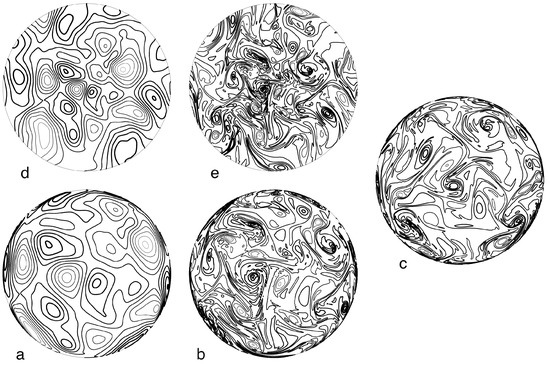
Figure 3. Stream function, (a,d), and vorticity, (b,c,e), at time $t=2.0$ in a non-rotating, viscous experiment in which the initial energy is confined to spherical harmonic degrees $n=16,17,18$. (a,b) are polar views, as seen by an observer at $z=\infty$, above the north pole. (d,e) are northern-hemisphere stereographic views that depict the same field as the polar views directly below. Compared to the polar views (a,b), the stereographic views (d,e) are relatively free of distortion. Panel (c) is an equatorial view, as seen by an observer at $x=\infty$. In all views, darker contour lines correspond to larger values.

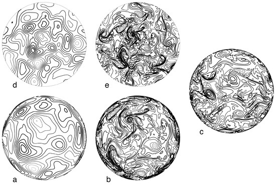
Figure 4. The same as Figure 3 but for the case $\Omega =50$ of Earth-like rotation. This solution differs from that of Figure 3 in that isolated coherent vortices are less prominent, and that elongated, jet-like structures are beginning to appear, especially near the equator in (c), where the $\beta$-effect is greatest.

In Figure 3 and Figure 4, (a) is a polar view of the stream function in the northern hemisphere, as seen by an observer at $z=\infty$ above the north pole, and (d) is the same field within the stereographic cirle ${\widehat{\xi }}^2+{\widehat{\eta }}^2<1$ corresponding to the northern hemisphere. Although both views cover the entire northern hemisphere, the polar view (a) hides features near the equator: the ratio between true distance and apparent distance in (a) varies between unity at the pole and infinity at the equator. In contrast, the stereographic view (d) introduces a scale distortion that varies only between 1 and 2. It offers the superior view of the entire northern hemisphere field.

Figure 4 shows the same 5 views as in Figure 3 but for the case $\Omega =50$ of non-vanishing angular momentum. Figure 4 differs from Figure 3 in that its isolated coherent vortices are less prominent than in Figure 3, and elongated, jet-like structures are beginning to appear, especially near the equator (Figure 4c), where the $\beta$-effect is greatest.

Figure 3 and Figure 4 illustrate the advantage of stereographic projection. Whereas at least six conventional views of the sphere are needed to give a fair representation of a single field, two stereographic projections offer a complete and relatively undistorted depiction.

Next, we consider two experiments, in which the initial state is sharply confined to spherical harmonics of degree $n=6$. Angular momentum corresponding to a solid body rotation rate $\Omega =50$ is present, but now it points in the direction of the y-axis in the Cartesian embedding space. This is achieved by replacing the Coriolis parameter f in (34) by

$$2\Omega y=2\Omega \frac{2\eta }{{\xi }^2+{\eta }^2+1}=2\Omega \frac{2\widehat{\eta }}{{\widehat{\xi }}^2+{\widehat{\eta }}^2+1}.$$

(82)

According to Section 3, the $n=6$ initial state should rotate rigidly, in a retrograde manner, about the y-axis at the angular rate $\omega \equiv 2\Omega /(6(6+1))$. Figure 5 shows this motion as seen by an observer at $x=\infty$. From its perspective, the pattern rotates upward in the figure, around the sphere, completing a full cycle of revolution in the recurrence time $2\pi /\omega =2.639$ shown on the far right of the figure. The solutions depicted in Figure 5 are both a check on the theory and a strong test of the numerical code because the rotation carries the pattern from the interior of one stereographic circle to the other and then back again, twice crossing the irregularly shaped elements near the bounding circles (11). The inviscid experiment (bottom row of Figure 5) exhibits small, grid-scale oscillations in the vorticity field, which do not appear in the viscous experiment (top row).

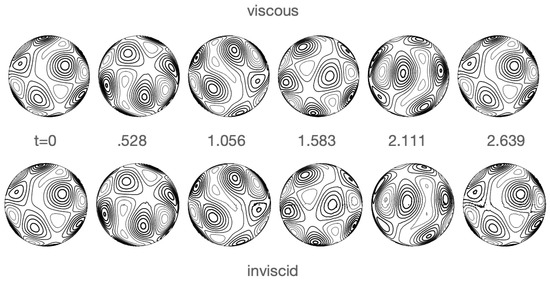
Figure 5. Vorticity as seen from $x=\infty$ at 6 times in two solutions in which the angular momentum vector points in the y-direction. z increases upward in the figure. The initial state at $t=0$ consists only of harmonics of degree $n=6$. The pattern rotates upward in the figure, around the sphere, to return to its original location at the predicted time $t=2.639$. The inviscid solution shows small, grid-scale oscillations in the vorticity that do not appear in the viscous solution.

Finally, we explore the suggestion in Section 1 that solutions lock into a static state as Bose–Einstein condensation occurs. Theory predicts Bose–Einstein condensation only as $n_c\to \infty$ and $t\to \infty$—two limits that are impossible to achieve numerically. The interesting question is whether quasi-static states appear with finite resolution and in finite time. According to equilibrium statistical mechanics [5], the equilibrium energy in spherical harmonic degree n is

$$E_n=\frac{2n+1}{\alpha +\beta n(n+1)},n\ge 2$$

(83)

where the constants $\alpha$ and $\beta$ are determined by the energy and enstrophy. The equilibrium spectrum (83) is the analogue of Kraichnan’s spectrum

$$E(k)=\frac{k}{\alpha +\beta k^2}$$

(84)

for flow on the plane [4]. The spectra (83) and (84) represent the final states attained by the inviscid, spectrally truncated dynamics after an indefinite period of adjustment. The numerator in (83) is the number of modes of degree n. Bose–Einstein condensation corresponds to the limit $\alpha \to -2(2+1)\beta$ as $n_c\to \infty$.

Several authors investigate freely decaying turbulence on the sphere and its resemblance to the predictions of equilibrium statistical mechanics, including the more recondite Miller–Sommeria–Robert–Montgomery (MRSM) theory ([26,27,28,29]). For a summary of the MRSM theory, see [30]. The requirement that $t\to \infty$ has proved formidable. MRSM theory claims to predict the structure of coherent vortices by the principle of maximum entropy. Ref. [31] offers a different picture, in which coherent vortices are low entropy sites that exist in order to maximize the rate of entropy production in the area outside the vortices.

Here, we consider the case $\Omega =\nu =0$ of non-rotating, inviscid flow with a modest resolution corresponding to $n_c=240$. The initial condition corresponds to energy distributed equally among the three degrees $n=4,5,6$, that is, $E_4=E_5=E_6$ with all other $E_n=0$. The amplitudes of the spherical harmonics within each band are randomly assigned, and the initial state is normalized such that $u_{rms}=1.$ A calculation based upon (83) predicts that 99.6% of the energy will end up in $n=2$, the lowest available mode. Again, $E_1=0$ at all time by the conservation of angular momentum. Figure 6 summarizes the evolution of the flow from $t=0$ to $t=60$. The time $t=60$ is the time required for a fluid particle to circumnavigate a great circle $60/2\pi =9.5$ times at the rms velocity of the flow. The dashed curve in Figure 6 is the fraction of energy in $n=2$. Beginning from zero, it only gradually approaches its predicted value of 0.996.

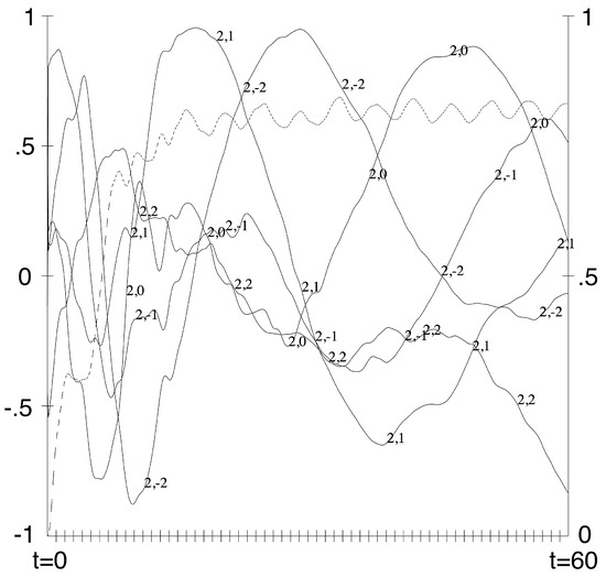
Figure 6. Evolution of a non-rotating, inviscid flow, in which the initial energy is confined to spherical harmonic degrees $n=4,5,6$. The dashed curve (right scale) is the fraction of energy in $n=2$, which vanishes initially, but, according to theory, will eventually reach 0.996. The other curves, labeled $2,m$, represent the normalized coefficient of $Y_2^m$ in the spherical harmonic representation of the flow, which vary between $\pm 1$ (left scale).

The solid curves in Figure 6 measure the approach to a static configuration. Let $A_{2,m}$ be the amplitude of $Y_2^m$ in the spherical harmonic representation of $\psi$, and define

$$\mathbf{p}=\frac{(A_{2,0},A_{2,1},A_{2,-1},A_{2,2},A_{2,-2})}{{\left[{(A_{2,0})}^2+{(A_{2,1})}^2+{(A_{2,-1})}^2+{(A_{2,2})}^2+{(A_{2,-2})}^2\right]}^{1/2}}.$$

(85)

Thus, $\mathbf{p}$ is a unit vector in the 5-dimensional space spanned by the amplitudes of the five spherical harmonics comprising $n=2$. If the flow were indeed to become static, then the five components of $\mathbf{p}$ would become time independent at values that are accidents of the initial conditions. Our choice of conventionally defined spherical harmonics as amplitudes to be tested is both arbitrary and irrelevant; any other choice of mutually orthogonal functions that span ${\psi }_2$ would serve as well.

Figure 6 shows that the approach to the putative equilibrium state is extremely slow. Although $E_2$ generally increases, its increase is not monotonic but instead exhibits persistent, relatively rapid oscillations. The components of $\mathbf{p}$, labeled $2,m$ in the figure oscillate over their full range of $\pm 1$, but the periods of their oscillations appear to lengthen as time increases. It is conceivable that this flow eventually reaches a static state, but this evidently requires a very long time. On the other hand, since the time unit is the time required for a fluid particle to move a distance equal to the radius of the sphere, the flow at $t=60$ is already quasi-static in the sense that it requires at least several such time units for the components of $\mathbf{p}$ to change appreciably.

6. Discussion

Spectral methods based upon the conventionally defined spherical harmonics in spherical coordinates are still probably the method of choice in atmosphere modeling. Norman Phillips [32] proposed the use of two stereographic coordinate systems to overcome the pole problem, but there remained the problem of matching the two stereographic systems together. Subsequent workers sandwiched a band of spherical or Mercator coordinates between separate stereographic regions at the poles ([33,34,35,36]), or omitted the band and interpolated between the two stereographic systems in an overlapping region near the equator [37]. In the present paper, we solve the stereographic equations within two non-overlapping circles and match the solutions on the circles themselves.

Our strategy requires the use of irregular quadrilaterals that conform to the circles, as shown in Figure 2. The existence of many irregular shaped equatorial elements is cause for concern, but none of our numerical experiments, including those depicted in Figure 3, Figure 4 and Figure 5, show evidence of spurious behavior near the equator. This good behavior is typical of Arakawa-type models that conserve energy and enstrophy when the viscosity vanishes.

Gridpoint methods outperform spectral methods when sharp features, such as boundaries, are present. Suppose that the spherical flow domain excluded an irregularly shaped island, or consisted of an ocean with an irregular boundary. It is very likely that our method of using quadrilaterals that conform to the equator would work equally as well for the boundary of the excluded region.

Compared to the plane, there are relatively few exact solutions for incompressible flow on the sphere. In fact, zonal flows and the solutions discussed in Section 3 seem to be the only exact analytical solutions for the sphere that do not contain point vortices or other singularities.

On the other hand, the solutions of Section 3 have no analogue on the plane because, as noted in Section 1, typical planar geometries do not correspond to many modes with the same wavenumber magnitude. In the commonly considered case of an infinitely periodic box, the modes correspond to integer pairs $(n,m)$, but relatively few of these occupy the same circle in the wavenumber plane. Circles with integral radius l contain the modes $(\pm l,0)$ and $(0,\pm l)$, but the circle contains the additional mode $(n,m)$ only if

$$n^2+m^2=l^2.$$

(86)

Integers $n,m,l$ that satisfy (86) are called Pythagorean Triples and are relatively sparse, the best known example being $3,4,5$. In contrast, there are $2n+1$ spherical harmonics with the same value of $n(n+1)$.

We associate the exact solutions of Section 3 with the rotational symmetry of the sphere, which corresponds by Noether’s theorem to angular momentum conservation. This symmetry is broken by all the usual planar geometries, including the infinitely periodic box, exceptions being the infinite plane and a perfectly circular domain. These facts only serve to underline the importance of angular momentum conservation in models, including by viscosity.

This paper advocates strongly in favor of stereographic coordinates for analysis, modeling, and flow visualization, but it is only fair to point out that different coordinate systems could be used for each of these purposes: one could use the cubed-sphere technique to perform the calculations, and still view the results in stereographic coordinates. We do admit a strong prejudice against spherical coordinates and the usual association between spherical coordinates and spherical harmonics. The latter are defined by the covariant property (54) and can be written in any system of coordinates.

References

- Herring, J.; Orszag, S.; Kraichnan, R.; Fox, D. Decay of two-dimensional homogeneous turbulence. J. Fluid Mech. 1974, 66, 417–444. [Google Scholar] [CrossRef]
- Herring, J.R. On the Statistical Theory of Two-Dimensional Topographic Turbulence. J. Atmos. Sci. 1977, 34, 1731–1750. [Google Scholar] [CrossRef]
- Herring, J.R. Statistical theory of quasi-geostrophic turbulence. J. Atmos. Sci. 1980, 37, 969–977. [Google Scholar] [CrossRef]
- Kraichnan, R.H. Inertial ranges in two-dimensional turbulence. Phys. Fluids 1967, 10, 1417–1423. [Google Scholar] [CrossRef]
- Frederiksen, J.; Sawford, B. Statistical dynamics of two-dimensional inviscid flow on a sphere. J. Atmos. Sci. 1980, 37, 717–732. [Google Scholar] [CrossRef]
- Kochin, N.E.; Kibeĺ, I.A.; Roze, N.V. Theoretical Hydromechanics; Interscience Publishers: New York, NY, USA, 1964. [Google Scholar]
- Rhines, P.B. Waves and turbulence on a beta-plane. J. Fluid Mech. 1975, 69, 417–443. [Google Scholar] [CrossRef]
- Vallis, G.K.; Maltrud, M.E. Generation of mean flows and jets on a beta plane and over topography. J. Phys. Oceanogr. 1993, 23, 1346–1362. [Google Scholar] [CrossRef]
- Boer, G.J.; Shepherd, T. Large-scale two-dimensional turbulence in the atmosphere. J. Atmos. Sci. 1983, 40, 164–184. [Google Scholar] [CrossRef]
- Sawford, B.; Frederiksen, J. Mountain torque and angular momentum in barotropic planetary flows: Equilibrium solutions. Q. J. R. Meteorol. Soc. 1983, 109, 309–324. [Google Scholar] [CrossRef]
- Egger, J.; Weickmann, K.; Hoinka, K.P. Angular momentum in the global atmospheric circulation. Rev. Geophys. 2007, 45, RG4007. [Google Scholar] [CrossRef]
- Gill, A.E. Atmosphere-Ocean Dynamics; Academic Press: New York, NY, USA, 1982. [Google Scholar]
- Gilbert, A.D.; Riedinger, X.; Thuburn, J. On the form of the viscous term for two dimensional Navier–Stokes flows. Q. J. Mech. Appl. Math. 2014, 67, 205–228. [Google Scholar] [CrossRef]
- Thompson, P.D. A generalized class of exact time-dependent solutions of the vorticity equation for nondivergent barotropic flow. Mon. Weather Rev. 1982, 110, 1321–1324. [Google Scholar] [CrossRef]
- Verkley, W. The construction of barotropic modons on a sphere. J. Atmos. Sci. 1984, 41, 2492–2504. [Google Scholar] [CrossRef]
- Salmon, R.; Talley, L.D. Generalizations of Arakawa’s Jacobian. J. Comput. Phys. 1989, 83, 247–259. [Google Scholar] [CrossRef]
- Needham, T. Visual Complex Analysis; Oxford University Press: Oxford, UK, 1997. [Google Scholar]
- Needham, T. Visual Differential Geometry and Forms: A Mathematical Drama in Five Acts; Princeton University Press: Princeton, NJ, USA, 2021. [Google Scholar]
- Becker, E.; Burkhardt, U. Nonlinear horizontal diffusion for GCMs. Mon. Weather Rev. 2007, 135, 1439–1454. [Google Scholar] [CrossRef]
- Jiménez, J. Hyperviscous vortices. J. Fluid Mech. 1994, 279, 169–176. [Google Scholar] [CrossRef]
- Rochas, M. Comments on “A Generalized Class of Time-Dependent Solutions of the Vorticity Equation for Nondivergent Barotropic Flow”. Mon. Weather Rev. 1984, 112, 390. [Google Scholar] [CrossRef]
- Neven, E. Quadrupole modons on a sphere. Geophys. Astrophys. Fluid Dyn. 1992, 65, 105–126. [Google Scholar] [CrossRef]
- Crowdy, D.G. Stuart vortices on a sphere. J. Fluid Mech. 2004, 498, 381–402. [Google Scholar] [CrossRef]
- Arakawa, A. Computational design for long-term numerical integration of the equations of fluid motion: Two-dimensional incompressible flow. Part I. J. Comput. Phys. 1966, 135, 103–114. [Google Scholar] [CrossRef]
- Salmon, R. A shallow water model conserving energy and potential enstrophy in the presence of boundaries. J. Mar. Res. 2009, 67, 779–814. [Google Scholar] [CrossRef]
- Qi, W.; Marston, J. Hyperviscosity and statistical equilibria of Euler turbulence on the torus and the sphere. J. Stat. Mech. Theory Exp. 2014, 2014, P07020. [Google Scholar] [CrossRef]
- Dritschel, D.G.; Qi, W.; Marston, J. On the late-time behaviour of a bounded, inviscid two-dimensional flow. J. Fluid Mech. 2015, 783, 1–22. [Google Scholar] [CrossRef]
- Modin, K.; Viviani, M. A Casimir preserving scheme for long-time simulation of spherical ideal hydrodynamics. J. Fluid Mech. 2020, 884, A22. [Google Scholar] [CrossRef]
- Jagad, P.; Samtaney, R. Effects of rotation on vorticity dynamics on a sphere with discrete exterior calculus. Phys. Fluids 2021, 33, 107117. [Google Scholar] [CrossRef]
- Eyink, G.L.; Sreenivasan, K.R. Onsager and the theory of hydrodynamic turbulence. Rev. Mod. Phys. 2006, 78, 87. [Google Scholar] [CrossRef]
- Salmon, R. Entropy budget and coherent structures associated with a spectral closure model of turbulence. J. Fluid Mech. 2018, 857, 806–822. [Google Scholar] [CrossRef]
- Phillips, N. A map projection system suitable for large-scale numerical weather prediction. J. Meteor. Soc. Jpn. 1957, 75, 262–267. [Google Scholar] [CrossRef]
- Phillips, N.A. Numerical integration of the primitive equations on the hemisphere. Mon. Weather Rev. 1959, 87, 333–345. [Google Scholar] [CrossRef]
- Chen, Y.; Kuo, H. A global model with overlapping mercator and stereographic grids. Adv. Atmos. Sci. 1986, 3, 302–313. [Google Scholar] [CrossRef]
- Browning, G.L.; Hack, J.J.; Swarztrauber, P.N. A comparison of three numerical methods for solving differential equations on the sphere. Mon. Weather Rev. 1989, 117, 1058–1075. [Google Scholar] [CrossRef]
- Lanser, D.; Blom, J.; Verwer, J. Spatial discretization of the shallow water equations in spherical geometry using Osher’s scheme. J. Comput. Phys. 2000, 165, 542–565. [Google Scholar] [CrossRef]
- Dudhia, J.; Bresch, J.F. A global version of the PSU–NCAR Mesoscale Model. Mon. Weather Rev. 2002, 130, 2989–3007. [Google Scholar] [CrossRef]
Disclaimer/Publisher’s Note: The statements, opinions and data contained in all publications are solely those of the individual author(s) and contributor(s) and not of MDPI and/or the editor(s). MDPI and/or the editor(s) disclaim responsibility for any injury to people or property resulting from any ideas, methods, instructions or products referred to in the content. |
© 2023 by the authors. Licensee MDPI, Basel, Switzerland. This article is an open access article distributed under the terms and conditions of the Creative Commons Attribution (CC BY) license (https://creativecommons.org/licenses/by/4.0/).