Abstract
NO3 radicals are one of the very important trace gases in the atmosphere. Accurate measurements of NO3 can provide data support for atmospheric chemistry research. Due to the extremely low content of NO3 radicals in the atmosphere, it is a challenge to accurately detect it. In this paper, an incoherent broadband cavity-enhanced absorption spectrometer (IBBCEAS) with high sensitivity is developed for measuring atmospheric NO3. The IBBCEAS absorption spectra of NO3 in the range of 648–674 nm are measured. The concentration of NO3 is retrieved by fitting the absorption cross-section of NO3 to the measured absorption coefficient using the least square method. The interference absorption of water vapor is effectively removed by an iterative calculation of its absorption cross-section. The detect limit of the spectrometer is analyzed using the Allan variance and the standard variance. The NO3 detection limit (1σ) of the spectrometer is 1.99 pptv for 1 s integration time, and improves to be 0.69 pptv and 0.21 pptv for 10 s and 162 s integration time, respectively. The developed spectrometer with pptv level sensitivity is applied to the measurements of the real atmospheric NO3 for verifying the effectiveness.
1. Introduction
The ability of the atmosphere to load and remove trace gases is the focus of atmospheric chemists. As a “cleaner” of the night atmosphere, NO3 radicals play an important role in atmospheric chemistry [1,2]. Although the content of NO3 in the atmosphere is extremely low, it determines the budget of some hydrocarbon substances at night, the most representative of which are isoprene and terpene [3]. Moreover, NO3 radicals affect the amount of NOx (NO and NO2) and VOCs at night and change the composition of aerosols [4,5,6]. The oxidation reaction between NO3 and VOCs as well as organic sulfides, together with the ozone decomposition of alkenes, is responsible for the generation and circulation of OH radicals and peroxy radicals (HO2 + RO2) at night [7]. In addition, the reaction of NO3 radicals with biological hydrocarbon will produce organic nitrate and secondary organic aerosol [8].
In order to clearly understand the nocturnal chemical process of NO3 radicals, sufficient and accurate atmospheric NO3 observation data must be available. Due to the extremely low content of NO3 radicals in the atmosphere, the NO3 concentration varies from several to hundreds of pptv at night [9], while the concentration is usually sub-pptv in the daytime owing to NO3 photolysis. At the same time, NO3 radicals also have high spatiotemporal characteristics, so it is very difficult to accurately detect them. Therefore, in order to realize the detection of NO3 radicals with high sensitivity and high time resolution, the detection technology is very demanding.
Since Platt and Noxon et al. [10,11] used differential optical absorption spectroscopy (DOAS) methods to measure NO3 radicals in the troposphere atmosphere for the first time in 1980, many relevant research groups have developed long path DOAS technology to carry out measurements of NO3 radicals in different atmospheric environments such as the land boundary layer [12], ocean boundary layer [13], urban area [14], and rural and forest area [15]. In addition to DOAS technology, the methods for measuring NO3 radicals mainly include laser-induced fluorescence spectroscopy (LIF) [16], cavity ring-down spectroscopy (CRDS) [17,18,19], and cavity-enhanced differential optical absorption spectroscopy (CEDOAS) [20,21]. Although the long path DOAS method is the most widely used, its measured NO3 concentration is the average concentration of NO3 distributed in the absorption optical path. Due to the rapid spatiotemporal variation of NO3, it cannot be guaranteed that NO3 is uniformly mixed at any time in the absorption optical path, resulting in that the measurement results cannot truly reflect the concentration distribution of NO3. Moreover, the long path DOAS method is subject to the weather and the measurement location; for example, it cannot work in snowy or foggy days, nor can it work on mobile platforms.
Incoherent broadband cavity-enhanced absorption spectroscopy (IBBCEAS) first proposed by Fiedler et al. [22] provides a new idea and method for the measurement of atmospheric NO3 radicals. First of all, IBBCEAS technology evolved from CRDS. It not only retains the high sensitivity detection performance of CRDS, but also simplifies the complexity of the CRDS device. Secondly, IBBCEAS technology uses an incoherent broadband light source, for example xenon lamp and light emitting diode (LED), as the light source of the measurement system, so it is a broadband absorption spectrum measurement technology. It uses a spectrometer to disperse the outgoing light of the optical cavity, and then uses CCD and other detectors to receive and convert the optical signal. The final result is a broadband absorption spectrum (usually tens of nanometers width) containing a variety of trace gas concentration information. That is, IBBCEAS technology can simultaneously measure many kinds of atmospheric trace gases, which is completely different from the single selective measurement of CRDS technology. Moreover, although the optical cavity used by IBBCEAS technology is similar to the CRDS optical cavity, it does not need to consider the mode matching, cavity length scanning or wavelength scanning when CRDS uses laser as the light source, and the requirements for the stability of the cavity are not very strict. Therefore, the IBBCEAS device is relatively simple and very suitable for field measurements. In addition, the measurement based on IBBCEAS is almost unaffected by the weather, and the measurement platform is considerably flexible, for example on the ground, tower, vehicle, ship and airborne. Especially and importantly, NO3 radicals measured by IBBCEAS technology are distributed in the point area, so it is easy to obtain the high spatiotemporal concentration change information of NO3 radicals in the local small-scale range. Other measuring instruments can be put together with IBBCEAS instruments to measure the relevant gases at the same location. Because the gas distribution areas measured by these instruments are the same, it is easy to combine their measurement data to help researchers analyze the atmospheric chemical and physical processes occurring in the measurement area.
In recent years, IBBCEAS technology has been widely used in the detection of gases with above ppbv concentrations in the atmosphere, for example NO2 [23,24,25,26,27,28,29,30,31,32,33], HONO [28,29,30,31,32,33,34,35,36], HCHO [36,37], CHOCHO [38,39,40,41,42], SO2 [43], and halogen oxides [44,45,46,47]. However, for the measurement of atmospheric NO3 radicals which have concentrations at the pptv level in the atmosphere, three orders of magnitude lower than ppbv, only a few studies have reported the application examples of IBBCEAS technology. For example, Venables et al. [48] measured the absorption of NO3 in the range of 645–675 nm using IBBCEAS technology with a xenon lamp as the light source. The detection sensitivity of NO3 reached 4 pptv in the spectrum acquisition time of 1 min, but they measured the NO3 generated by the reaction of NO2 and O3 in an atmospheric simulation chamber, not the NO3 in the actual atmosphere. Subsequently, they established an open optical path IBBCEAS device with a long optical cavity (cavity length of 20 m) for measuring NO3, NO2 and aerosol extinction [49]. The detection sensitivity of NO3 reached 2 pptv in the spectrum acquisition time of 5 s; however, the measurement object was still a simulated atmosphere. Similarly, Yi et al. [50,51] and Wu et al. [52] used the IBBCEAS to implement the measurements of NO3 in the atmospheric simulation chamber. Langridge et al. [53] developed an LED light source-based IBBCEAS instrument to measure NO3 radicals (including NO3 generated by the thermal decomposition of N2O5) in the marine boundary layer during the RHaMBLe field campaign at Roscoff, France. The detection sensitivity reached 0.25 pptv when the acquisition time was 10 s. Shortly afterwards, they carried out the observation experiments of NO3, N2O5 and NO2 using an airborne platform-based IBBCEAS instrument [54]. The observation results verified that IBBCEAS technology can realize the rapid measurement of atmospheric trace gases as well as obtain high spatiotemporal concentration change information of NO3 radicals. Additionally, Nam et al. [55] developed an IBBCEAS spectrometer for simultaneous measurements of ambient NO3, NO2 and H2O. Wang et al. [56] developed a red LED-based IBBCEAS instrument for measuring the sum of NO3 and N2O5 in a polluted urban environment. The NO3 detection limit was about 2.4 pptv and 1.6 pptv for the acquisition time of 1 s and 30 s, respectively. Measuring the absorption of the sum of NO3 and N2O5 is easier than measuring that of NO3 alone. Moreover, they used a NO titration method to remove the absorption structure of water vaper. Duan et al. [57] developed a similar IBBCEAS instrument for measuring ambient NO3 in Hefei city, China. The average concentration of the measured NO3 was ~11.6 pptv at night and the NO3 detection limit was about 0.75 pptv for the acquisition time of 10 s. They used the measured spectrum in the daytime as the reference spectrum to reduce the absorption interference of water vapor. However, whether using NO titration or a daytime reference spectrum to remove the interference of water vapor, it virtually leads the IBBCEAS instrument to lose the ability of the simultaneous measurement of other trace gases, for example NO2, thus losing the advantages of IBBCEAS technology in broadband measurement over CRDS technology. In addition, Suhail et al. [58] and Wang et al. [59] used open path incoherent broadband cavity-enhanced absorption spectroscopy (OP-IBBCEAS) to detect NO3 radicals in the atmosphere. However, the detection sensitivity of NO3 deteriorates due to unavoidable aerosol extinction, which leads to a larger detection limit compared with closed path IBBCEAS.
In this paper, we develop an IBBCEAS instrument with pptv level sensitivity for measuring atmospheric NO3. The main contributions of this work include the following. (1) The improvement of the detection limit for NO3 by designing the mechanical assembly, based on a four-rod cage system, is made. Mechanical assembly and high reflectivity mirrors make the optical path length up to 7.6 km even if the cavity length is only 50 cm, which ensures the measurement sensitivity of the instrument. (2) Our instrument has the ability to simultaneously measure multiple species, i.e., NO3, NO2 and H2O, because the interference absorption of water vapor is effectively removed by iteratively calculating its cross-section instead of using the reference spectrum recorded in the daytime or using the NO titration method. (3) The NO3 detection limit (1σ) of our instrument is improved to be 0.69 pptv for the integration time of 10 s, which is lower compared with the existing IBBCEAS instruments which have a hardware configuration similar to that of our instrument. The improvement of the instrument performance depends on the optical path design, mechanical assembly and certainly high reflectivity of cavity mirrors.
The rest of this paper is organized as follows. Section 2 introduces the IBBCEAS principle and instrument. Section 3 describes the calibration of the mirror reflectivity and the calibration of the effective cavity length. Section 4 shows the spectrum retrieval, and discusses the transmission efficiency of NO3, the stability, uncertainty and detection limit of the instrument as well as real applications. Finally, Section 5 summarizes the conclusions.
2. The Principle and Instrument
2.1. The Principle of IBBCEAS
IBBCEAS technology uses an optical cavity for letting the incident light to form multiple reflections in the cavity to increase the optical path and thus improve the detection sensitivity. Fiedler et al. [22] described the principle of quantifying trace gas concentrations with IBBCEAS. The absorption coefficient of the measured gases can be expressed as:
where and are the absorption cross-section and the number density for species i, respectively, is the absorption coefficient of the measured gases, d is the optical cavity length, is the reflectivity of cavity mirrors, and and are the measured spectra with and without absorbing species in the cavity, respectively. The number density of the measured objects can be retrieved by fitting the absorption cross-sections to the absorption coefficient.
2.2. The IBBCEAS Instrument
2.2.1. Optical Layout
The schematic diagram of the IBBCEAS instrument is shown in Figure 1a. The instrument is composed of a red light emitting diode (LED), two lenses, two plane-concave mirrors, a spectrometer and a gas cell. The core of the instrument is the optical cavity that is formed by plane-concave mirrors M1 and M2. M1 (or M2) has high reflectivity and the calibrated reflectivity by the manufacturer is more than 0.9999 within 640–680 nm. The diameter and radius curvature of the high reflectivity (HR) mirror are 25 mm and 1 m, respectively. The distance between M1 and M2, i.e., the optical cavity length, is 50 cm. In order to avoid being contaminated by the measured sample, both mirrors M1 and M2 are continuously purged by clean nitrogen flow. The red LED, which has a center wavelength of 660 nm at 20 ℃ and full width at half maximum (FWHM) of 26 nm, is regarded as the light source for exciting the optical cavity. Considering the influence of working current and temperature on the stability of the emitting spectrum, the red LED is driven by a constant current of 1000 mA. In addition, a thermoelectric cooler with a control unit is used to keep the LED temperature stable at 25 ℃. The reason why the LED temperature is selected to be stable at 25 ℃ is that its center wavelength can match with the absorption peak wavelength of NO3 (~662nm) by increasing the LED temperature. The lens L1 (f = 20 mm, diameter = 25 mm) is used to collimate the red light into the optical cavity. The light exiting from the optical cavity is focused by another lens, i.e., L2 (f = 50 mm, diameter = 25 mm), on one end of a fiber while the other end is connected to a spectrometer. The diameter and numerical aperture (NA) of the fiber are 400 μm and 0.22, respectively. The spectrometer is from Ocean Optics in the USA and the type is QE65Pro, of which the entrance slit width, line density of the diffraction grating and spectral resolution in the wavelength range of 640–720 nm are 200 μm, 1800 mm−1 and 0.9 nm, respectively. The detailed specifications of all the optical components used in the IBBCEAS instrument are listed in Table 1. The mechanical assembly of the instrument is based on a four-rod cage system as shown in Figure 1b, which ensures the collimation and stability of the optical path.
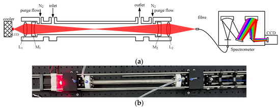
Figure 1.
The schematic diagram and photograph of the IBBCEAS instrument. (a) The schematic diagram of the IBBCEAS instrument; (b) a photograph of the instrument. The mechanical assembly is based on a four-rod cage system.

Table 1.
The specifications of the optical components used in the IBBCEAS instrument.
2.2.2. Gas Flow System
The schematic diagram of the IBBCEAS instrument gas flow system is shown in Figure 2. The flow system is designed for calibrating the mirror reflectivity and the effective cavity length, purging the HR (M1, M2) and sampling the ambient air. The flow system consists of one aerosol filter, six valves (V1-V6), three mass flow controllers (MFC1, MFC2 and MFC3), one sample cell, one pressure meter, one temperature and humidity meter, three kinds of gases (N2, He and NO2/N2), one gas pump and a certain number of perfluoroalkoxy alkanes (PFA) tubes. The sample cell (exclude connectors at both ends) is one 35 cm long PFA tube, with inner and outer diameters of 10 mm and 12 mm, respectively, and is enclosed by a stainless tube, as shown in Figure 1b.
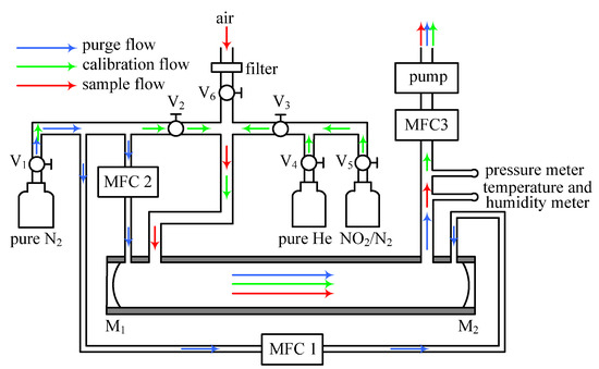
Figure 2.
The schematic diagram of the IBBCEAS instrument gas flow system. The blue arrow denotes N2 purge gas flow to prevent HR (M1, M2) from particle contamination. The green arrow denotes calibration gas flow for determining the mirror reflectivity and the effective cavity length. The red arrow denotes sample gas flow, namely the measured ambient air.
The diameters of the purging and sampling gas hole are 3 mm and 5 mm, respectively. Before pumping the ambient air into the sample cell, the mirror reflectivity and the effective cavity length often need to be calibrated (details of how to calibrate are given in Section 3.1 and Section 3.2). When calibrating the mirror reflectivity or the effective cavity length, both purge flow (blue arrow) and sample flow (red arrow) remain impassable by turning off MFC1 and MFC2, and closing V6. When sampling the ambient air, the calibration flow (green arrow) stops working (by closing V2 and V3), but the purge flow needs to be open. The flow rates of the sample and purge flow are 2 SLPM (standard liter per minute) and 0.2 SLPM, respectively.
3. Calibration
3.1. Calibration of the Mirror Reflectivity
Calibrating the mirror reflectivity is a very import procedure for incoherent broadband cavity-enhanced absorption spectroscopy. According to Equation (1), the absorption coefficient of the measured gases can only be obtained if the mirror reflectivity, , is known. In our previous work [26], we make use of the difference of Rayleigh scattering cross-sections between high-purity nitrogen and helium to calibrate the mirror reflectivity. In this paper, we still use this method to obtain the profile of the mirror reflectivity. As shown in Figure 3, open V1, V2 and MFC3, and close the remaining valves and MFCs. The sample cell is flushed with nitrogen with a purity of 99.999% with a flow rate of 2 SLPM. Measure the intensity of the transmitted light and record it as . Next, open V3, V4 and MFC3, and close the remaining valves and MFCs. The sample cell is flushed with helium with a purity of 99.999% with a flow rate of 2 SLPM. Measure the intensity of the transmitted light and record it as . The relative mirror reflectivity can be obtained according to the following equation [41]:
where and are the Rayleigh scattering extinction coefficient of nitrogen and helium, respectively, and is the cavity length. is equal to the product of nitrogen purity and nitrogen Rayleigh scattering cross-sections [60]. Additionally, is equal to the product of helium purity and helium Rayleigh scattering cross-sections [61]. Because ref. [60] and [61] only provided Rayleigh scattering cross-sections of nitrogen and helium at a specific wavelength, respectively, Rayleigh scattering cross-sections, , is interpolated to obtain cross-section values over the region of interest based on wavelength dependence to an expression ().
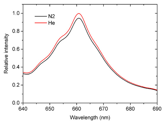
Figure 3.
The measured absorption spectra when the sample cell is flushed with nitrogen and helium both with purity of 99.999%, respectively.
Figure 3 shows the measured absorption spectra of high-purity nitrogen and helium, namely and . It can be seen that there is a distinct differentiation between and , which is owing to the fact that the Rayleigh scattering cross-sections of nitrogen (10−27 cm2/molecule level) is much larger than that of helium (10−29 cm2/molecule level) in the range of 640–690 nm.
According to Equation (2), we use and in Figure 3 to calculate the mirror reflectivity. Figure 4 shows the calibrated mirror reflectivity as well as the cavity loss. The black line is the calculated mirror reflectivity and the red line is the cubic polynomial fitting curve of the calculated mirror reflectivity. There is a maximum mirror reflectivity of 0.999934 at the wavelength of 665 nm. The orange line is the calculated cavity loss, namely (1 − , and the green line is the cubic polynomial fitting curve of the calculated cavity loss. There is a minimum cavity loss of 1.31 × 10⁻⁶ cm−1 at the wavelength of 665 nm, which corresponds to the optical path length of 7.6 km.
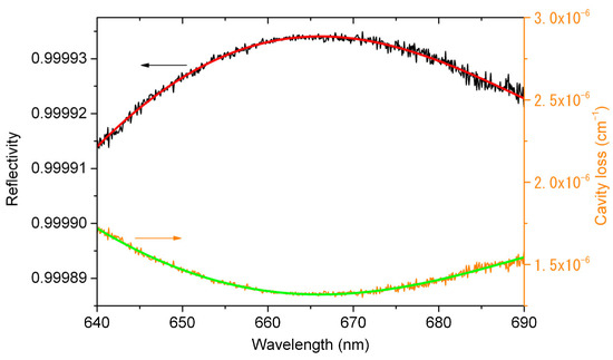
Figure 4.
The calculated mirror reflectivity (black line), the cubic polynomial fitting curve of the calculated mirror reflectivity (red line), the calculated cavity loss (orange line) and the cubic polynomial fitting curve of the calculated cavity loss (green line). The maximum mirror reflectivity is 0.999934 at 665 nm, and the corresponding cavity loss and optical path length are 1.31 × 10⁻⁶ cm−1 and 7.6 km, respectively.
3.2. Calibration of the Effective Cavity Length
The effective cavity length, , denotes the cavity length occupied by the sampling gases. At two ends of the cavity, we design a continuous purge gas flow to prevent the sampling gases from contaminating HR mirrors. The effective cavity length therefore is usually shorter than the distance ( is 50 cm in our instrument) between two HR mirrors, and longer than the distance ( is 40 cm in our instrument) between the sample inlet and outlet. In order to calibrate the , with and without purge gas flow, we pump a NO2 standard gas of 500 ppbv into the cavity, respectively. Measure the respective absorption spectrum and then retrieve the NO2 concentration by fitting NO2 cross-sections (obtained by the convolution of high-resolution NO2 cross-sections from ref. [62] with the instrument function of the spectrometer) to the measured absorption coefficient based on Equation (1), recording the retrieved NO2 number density as and , respectively. The is determined by the following equation:
Figure 5a shows the fitting example of NO2 standard gas when the purge gas flow is on. The resulting number density of NO2 is 455 ppbv. Figure 5b shows the measurement results of NO2 standard gas including the results with and without purge gas flow. The averages of and are 457 ppbv and 491 ppbv, respectively. The calculated is ~46.5 cm.
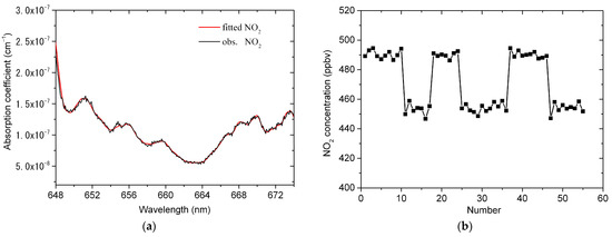
Figure 5.
Calibration of the effective cavity length. (a) An example of fitting one absorption spectrum of NO2 standard gas. The resulting number density of NO2 is 455 ppbv; (b) the measurement results of NO2 standard gas including the results with and without purge gas flow.
4. Results and Discussion
4.1. Spectrum Retrieval
The number density of NO3 radicals is retrieved from the measured spectra by the least squares fitting technique. The determination of the spectral fitting window is of importance for broadband absorption spectroscopy. After repeated testing and comparison, the range of 648–674 nm is regarded as the optimal fitting window. In addition to the absorption of NO3, there are the absorptions of other gases, for example NO2 and water vapor, in the wavelength range of 648–674 nm. Hence, the measured absorption coefficient can be approximated as:
where , and are the cross-sections of NO3, NO2 and water vapor, respectively, and , and are the number density of NO3, NO2 and water vapor, respectively.
Before the spectral fitting procedure starts, , and must be determined. is determined by the convolution of high-resolution NO3 cross-sections from ref. [63] with the instrument function of the spectrometer. Additionally, is determined by the convolution of high-resolution NO2 cross-sections from ref. [62] with the instrument function of the spectrometer. However, the water vapor’s absorption lines in the polyad have pressure-broadened half-widths of only 0.1 cm−1, which correspond to ~0.008 nm FWHM at 652 nm [64]. It means that the convolution method is inapplicable to get due to the fact that the resolution of our spectrometer (is 0.9 nm FWHM), far lower compared with the width of the water vapor’s absorption lines. In this paper, we use iterative calculation to obtain the effective cross-sections of water vapor. This method was also used by Kennedy et al. [54]. Figure 6 shows the procedure of iterative calculation for obtaining the effective .
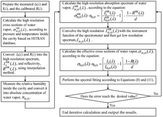
Figure 6.
The procedure of iterative calculation for obtaining the effective cross-sections of water vapor.
As shown in Figure 6, the procedure of an iterative calculation for obtaining the effective cross-sections of water vapor is as follows:
Step 1: Prepare the measured (reference and absorption) spectra and calibrated mirror reflectivity as the input of iterative calculation. The high-resolution cross-section of water vapor, , is calculated using the line-by-line parameters from the HITRAN database [65] as well as combining with the measured pressure and temperature inside the cavity.
Step 2: The low resolution and are converted into the high resolution and by applying interpolation.
Step 3: The high resolution absorption spectrum of water vapor,, is calculated using the measured concentration of water vapor,, according to the following equation:
Step 4: The low resolution absorption spectrum of water vapor,, is obtained by convolving the with the instrument function of the spectrometer.
Step 5: The effective cross-section of water vapor,, is calculated according to the following equation:
Step 6: Perform the spectral fitting according to Equations (1) and (4).
Step 7: Evaluate whether the error of the resulting water vapor concentration reaches the desired value. If yes, end the iterative calculation. Otherwise, back to step 3. In step 3, the is replaced by the water vapor concentration obtained from the previous spectral fitting.
Figure 7 shows an example of fitting one absorption spectrum measured in an ambient atmosphere. The acquisition time of the measured spectrum is 5 s, corresponding to the average of ten spectra and the exposure time of 500 ms for each spectrum. The black line in Figure 7a is the observed absorption coefficient including the absorption information of NO3, NO2, water vapor and other unknown species, and the red line is the fitted absorption coefficient. Figure 7b–d show the fitting results of NO3, NO2 and water vapor, respectively. It can be seen from Figure 7b that the absorption of NO3 is obviously observed by our developed instrument. The resulting number density of NO3 is 41.4 pptv and the fitting uncertainty is 1.6 pptv. Moreover, the absorption of NO2 is observed as shown in Figure 7c, which means that our instrument fully exploits the ability of broadband absorption spectroscopy to detect multiple species. Figure 7d shows that the interference absorption of water vapor in the measured spectrum has been effectively removed, which demonstrates the effectiveness of iteratively calculating the absorption cross-section of water vapor. Figure 7e shows the total fitting curve of the absorption coefficient including the second-order polynomial. The fitting residual is shown in Figure 7f and the standard deviation of the residual is 1.97 × 10⁻⁹ cm−1.
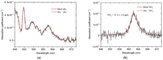
Figure 7.
An example of fitting one absorption spectrum measured in ambient atmosphere. The absorption spectrum is recorded with an acquisition time of 5 s (exposure time of 500 ms, 10 times average). (a) The observed (black line) and fitted (red line) absorption coefficient; (b) the observed (black line) and fitted (red line) NO3 absorption. The number density of NO3 is 41.4 ± 1.6 pptv; (c) The observed (black line) and fitted (red line) NO2 absorption. The number density of NO2 is 86.2 ± 5.1 ppbv; (d) the observed (black line) and fitted (red line) H2O absorption. The number density of H2O is 0.15%; (e) the total (black line) and fitted (red line) absorption coefficient, as well as the second-order polynomial; (f) residual spectrum with a standard deviation of 1.97 × 10⁻⁹ cm−1.
4.2. Transmission Efficiency of NO3
The wall loss and filter loss will deteriorate the transmission efficiency of NO3. The inlet and the sample cell in our instrument are constructed of a PFA tube. The inner diameter of the PFA tube is similar to that of the PFA tubes used in ref. [56] and in our previous work of measuring NO3 and N2O5 using CRDS [66]. According to the wall loss reported in refs. [56,66], we estimate the wall loss to be (20 ± 5%). The filter loss has been determined in our previous work [66], and is (17 ± 5%) for a clean filter while it increases to (19 ± 5%) for a used filter for 2 h. Overall, the transmission efficiency of NO3 is about (66 ± 8%) for a new filter. During the measurement process, we replace the filter every 2 h.
4.3. Stability, Uncertainty and Detection Limit Analysis
The stability of an instrument influences its sensitivity. Theoretically, high sensitivity can be achieved by signal averaging with a sufficient number of times. However, it is not true that the more the average number of times, the higher the sensitivity. In fact, a detection system only remains stable for a certain period of time. In this paper, we use the Allan variance method to determine the optimal integration time of the IBBCEAS instrument. Moreover, standard variance is used to determine the detection limit for NO3.
A data set about absorption spectra is created using 6000 consecutive measurements of when the sample cell is flushed with nitrogen (integration time of 1s each measurement, the total measurement time of 1.67 h). This data set is processed to produce a time series of spectra averaged over integration times ranging from 1 to 1000 s. In other words, we get a series of M = 6000 spectra with an integration time of 1 s, a series of M = 3000 spectra with an integration time of 2 s, and so on. The reason for determining the maximum integration time of 1000 s is to ensure that each series of spectra contain at least six averaged spectra. Each series of absorption coefficients are calculated according to Equation (1), and then individual series of the NO3 number density are obtained by fitting the cross-section of NO3 to these absorption coefficients. The Allan variance,, and the standard variance,, of each time series can be expressed as:
where for i = 1 to i = M is the NO3 number density in the time series of a given integration time, , and is the average value of the NO3 number density of the whole time series.
The square root of the Allan variance, named the Allan deviation , provides an indication of an instrument’s stability [67]. The red line in Figure 8a plots the relationship between the Allan deviation and the integration time. It can be observed that the Allan deviation decreases rapidly as the integration time increases from 1 s to 162 s. After the integration time is longer than 162 s, the Allan deviation begins to increase gradually, which indicates that further increasing the integration time does not improve the sensitivity of the instrument because it is difficult to ensure that the LED emission spectrum keeps stable for a long time. In order to reduce the influence of the variation in the LED emission spectrum on the instrument, it is advisable to measure a new reference spectrum the optimal integration time (162 s) later when the instrument works in the field campaign. Figure 8b shows the time series of NO3 concentration (number density) for the integration time of 1 s, 10 s and the optimum (162 s). It can be evidently seen that the peak-to-peak of the NO3 concentration decreases with the increase of the integration time, which indicates the noise can be effectively reduced by averaging spectra due to the fact that white noise dominates in the noise for < 162 s.
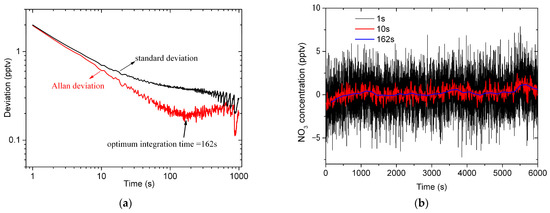
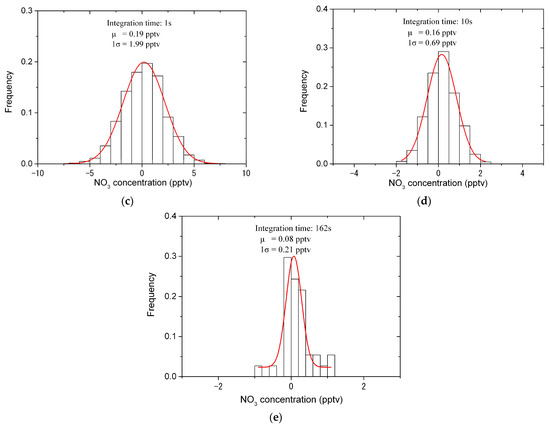
Figure 8.
Allan variance and standard variance for analyzing the stability and the detection limit of the IBBCEAS instrument. (a) The Allan deviation (red line) and the standard deviation (black line) for different integration times; (b) the time series of NO3 concentration (number density) for the integration time of 1 s (black line), 10 s (red line) and 162 s (blue line); (c) the histogram analysis of the time series of NO3 concentration for the integration time of 1 s. The detection limit of 1σ is 1.99 pptv; (d) the histogram analysis of the time series of NO3 concentration for the integration time of 10 s. The detection limit of 1σ is 0.69 pptv; (e) the histogram analysis of the time series of NO3 concentration for the integration time of 162 s. The detection limit of 1σ is 0.21 pptv.
The square root of the standard variance, named the standard deviation , provides an indication of an instrument’s detection limit [18,67] for a given integration time. The black line in Figure 8a plots the relationship between the standard deviation and the integration time. In the regime of white noise absolutely dominating in the noise (for < 5 s), the standard deviation and the Allan deviation are almost equivalent, but there is a considerable difference between them for > 5 s. Figure 8c–e show the histogram analysis of the time series of NO3 concentration (number density) for the integration time of 1 s, 10 s and the optimum (162 s), respectively. The detection limit of the instrument is 1.99 pptv (1σ) for the 1 s integration time, and improves to be 0.69 pptv (1σ) and 0.21 pptv (1σ) for the 10 s and 162 s integration time, respectively. Table 2 shows the comparison of our instrument’s detection limit with that of other instruments. Compared with the IBBCEAS instruments (for example, developed in refs. [56,57]) with the similar hardware configuration to our instrument, the detection limit of our instrument is lower.
Table 2.
Comparison of our instrument’s detection limit (1σ) with that of other instruments.
The uncertainty of the instrument mainly comes from the uncertainty of the NO3 cross-section (10%), the uncertainty of the mirror reflectivity (5%), the uncertainty of the effective cavity length (6%) and the uncertainty of the transmission efficiency of NO3 (8%). According to the error transfer rule, the uncertainty of our instrument for measuring NO3 is estimated to be 15%. It should be noted that it will lead to a large fitting uncertainty if the accurate water vapor concentration cannot be retrieved because the absorption structure of water vapor has not been effectively removed from the measured absorption coefficient.
4.4. Atmospheric NO3 Measurement
The developed instrument is applied to the measurements of real atmospheric NO3 to further verify its usefulness. The instrument is placed in a laboratory on the second floor of Anhui University of Science and Technology. The air sampling point is ~3 m high from the ground. A 1.5 m long PFA tube for sampling air connects to one end of the filter and the other end connects to the inlet of the sample cell. The flow rate of sampling air is set as 2 SLPM. The filter is replaced by a new one every two hours. The measurement of atmospheric NO3 was implemented from 19:00 on 16 January to 05:00 on 17 January in 2023, and the total measurement time is 10 h, corresponding to 7200 absorption spectra (5 s each spectrum). Figure 9 shows the time series of the measured atmospheric NO3 concentration, corrected by the transmission efficiency of NO3, and shows the estimated uncertainty. The number density of atmospheric NO3 ranges from −0.6 pptv to 44.2 pptv. The negative concentration is meaningless, which indicates the measured NO3 concentration is close to the detection limit of the instrument.
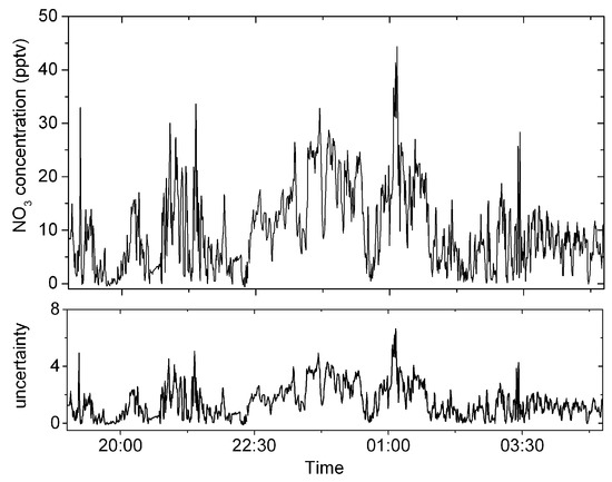
Figure 9.
The top panel shows the time series of the measured atmospheric NO3 concentration from 19:00 on January 16 to 05:00 on January 17 in 2023. The lower panel is estimated uncertainty.
In addition, the concentrations of NO2 and H2O are simultaneously retrieved for accounting for the advantage of the broadband technique. Figure 10a,b show the concentrations of NO2 and H2O, respectively.
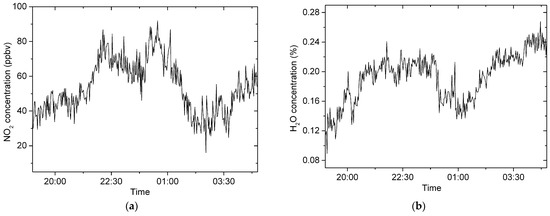
Figure 10.
The concentrations of NO2 and H2O from 19:00 on 16 January to 05:00 on 17 January in 2023. (a) NO2 concentrations; (b) water vapor concentrations.
5. Conclusions
In this paper, a pptv level incoherent broadband cavity-enhanced absorption spectrometer is developed for the measurement of atmospheric NO3. With a cavity length of 50 cm, the optical path reaches 7.6 km, and the NO3 detection limit of the developed instrument improved to be 0.69 pptv for the integration time of 10 s. Iteratively calculating the cross-section of the water vapor to remove its absorption interference ensures the instrument’s ability of simultaneous measurement of multiple species. The application of the instrument in the real measurements of atmospheric NO3 verifies the effectiveness and practicability.
Author Contributions
Methodology, L.L.; software, L.L. and W.L.; validation, L.L., W.L. and Q.Z.; investigation, W.L.; resources, Q.Z.; data curation, W.L.; writing—original draft preparation, W.L.; writing—review and editing, L.L.; visualization, W.L.; supervision, L.L.; project administration, L.L. All authors have read and agreed to the published version of the manuscript.
Funding
This research was supported in part by Anhui Province Key R&D Program of China under grant 202004i07020011, in part by Academic Support Project for Top-notch Talents in Disciplines (Majors) of Colleges and Universities in Anhui Province under grant gxbjZD2021052.
Institutional Review Board Statement
Not applicable.
Informed Consent Statement
Not applicable.
Data Availability Statement
Upon request data can be obtained from the authors.
Acknowledgments
In this section, you can acknowledge any support given which is not covered by the author contribution or funding sections. This may include administrative and technical support, or donations in kind (e.g., materials used for experiments).
Conflicts of Interest
The authors declare no conflict of interest.
References
- Zhang, C.X.; Sun, X.M.; Tan, W.; Peng, H.J. Atmospheric oxidation of Folpet initiated by OH radicals, NO3 radicals, and O3. RSC Adv. 2021, 11, 2346–2352. [Google Scholar] [CrossRef] [PubMed]
- Docherty, K.S.; Ziemann, P.J. Reaction of oleic acid particles with NO3 radicals: Products, mechanism, and implications for radical-initiated organic aerosol oxidation. J. Phys. Chem. A 2006, 110, 3567–3577. [Google Scholar] [CrossRef]
- Stutz, J.; Wong, K.W.; Lawrence, L.; Ziemba, L.; Flynn, J.H.; Rappengluck, B.; Lefer, B. Nocturnal NO3 radical chemistry in Houston, TX. Atmos. Environ. 2010, 44, 4099–4106. [Google Scholar] [CrossRef]
- Perraud, V.; Bruns, E.A.; Ezell, M.J.; Johnson, S.N.; Greaves, J.; Finlayson-Pitts, B.J. Identification of organic nitrates in the NO3 radical initiated oxidation of alpha-pinene by atmospheric pressure chemical ionization mass spectrometry. Environ. Sci. Technol. 2010, 44, 5887–5893. [Google Scholar] [CrossRef]
- Kerdouci, J.; Picquet-Varrault, B.; Doussin, J.F. Structure-activity relationship for the gas-phase reactions of NO3 radical with organic compounds: Update and extension to aldehydes. Atmos. Environ. 2014, 84, 363–372. [Google Scholar] [CrossRef]
- DeVault, M.P.; Ziola, A.C.; Ziemann, P.J. Products and mechanisms of secondary organic aerosol formation from the NO3 radical-initiated oxidation of cyclic and acyclic monoterpenes. ACS Earth Space Chem. 2022, 6, 2076–2092. [Google Scholar] [CrossRef]
- Bates, K.H.; Burke, G.J.P.; Cope, J.D.; Nguyen, T.B. Secondary organic aerosol and organic nitrogen yields from the nitrate radical (NO3) oxidation of alpha-pinene from various RO2 fates. Atmos. Chem. Phys. 2022, 2, 1467–1482. [Google Scholar] [CrossRef]
- Fan, M.Y.; Zhang, Y.L.; Lin, Y.C.; Hong, Y.H.; Zhao, Z.Y.; Xie, F.; Du, W.; Cao, F.; Sun, Y.L.; Fu, P.Q. Important role of NO3 radical to nitrate formation aloft in yrban Beijing: Insights from triple oxygen isotopes measured at the tower. Environ. Sci. Technol. 2022, 56, 6870–6879. [Google Scholar] [CrossRef]
- Brown, S.S.; Dube, W.P.; Peischl, J.; Ryerson, T.B.; Atlas, E.; Warneke, C.; de Gouw, J.A.; Hekkert, S.L.; Brock, C.A.; Flocke, F.; et al. Budgets for nocturnal VOC oxidation by nitrate radicals aloft during the 2006 Texas Air Quality Study. J. Geophys. Res. 2011, 116, D24305. [Google Scholar] [CrossRef]
- Platt, U.; Perner, D.; Winer, A.M.; Harris, G.W.; Pitts, J.N., Jr. Detection of NO3 in the polluted troposphere by differential optical absorption. Geophys. Res. Lett. 1980, 7, 89–92. [Google Scholar] [CrossRef]
- Noxon, J.F.; Norton, R.B.; Marovich, E. NO3 in the troposphere. Geophys. Res. Lett. 1980, 7, 125–128. [Google Scholar] [CrossRef]
- Geyer, A.; Ackermann, R.; Dubois, R.; Platt, U. Long-term observation of nitrate radicals in the continental boundary layer near Berlin. Atmos. Environ. 2001, 35, 3619–3631. [Google Scholar] [CrossRef]
- McLaren, R.; Wojtal, P.; Majonis, D.; Mccourt, J.; Halla, J.D.; Brook, J. NO3 radical measurements in a polluted marine environment: Links to ozone formation. Atmos. Chem. Phys. 2010, 10, 4187–4206. [Google Scholar] [CrossRef]
- Li, S.W.; Liu, W.Q.; Xie, P.H.; Yang, Y. Observation of nitrate radical in the nocturnal boundary layer during a summer field campaign in Pearl River Delta, China. Terr. Atmos. Ocean. Sci. 2012, 23, 39–48. [Google Scholar] [CrossRef] [PubMed]
- Geyer, A.; Alicke, B.; Mihelcic, D.; Stutz, J.; Platt, U. Comparison of tropospheric NO3 radical measurements by differential optical absorption spectroscopy and matrix isolation electron spin resonance. J. Geophys. Res. 1999, 104, 26087–26105. [Google Scholar] [CrossRef]
- Wood, E.C.; Wooldridge, P.J.; Freese, J.H.; Albrecht, T.; Cohen, R.C. Prototype for in situ detection of atmospheric NO3 and N2O5 via laser-induced fluorescence. Environ. Sci. Technol. 2003, 37, 5732–5738. [Google Scholar] [CrossRef]
- Wang, D.; Hu, R.Z.; Xie, P.H.; Liu, J.G.; Liu, W.Q.; Qin, M.; Ling, L.Y.; Zeng, Y.; Chen, H.; Xing, X.B.; et al. Diode laser cavity ring-down spectroscopy for in situ measurement of NO3 radical in ambient air. J. Quant. Spectrosc. Radiat. Transf. 2015, 166, 23–29. [Google Scholar] [CrossRef]
- Simpson, W.R. Continuous wave cavity ring-down spectroscopy applied to in situ detection of dinitrogen pentoxide (N2O5). Rev. Sci. Instrum. 2003, 74, 3442–3452. [Google Scholar] [CrossRef]
- Lin, C.; Hu, R.Z.; Xie, P.H.; Lou, S.R.; Zhang, G.X.; Tong, J.Z.; Liu, J.G.; Liu, W.Q. Nocturnal atmospheric chemistry of NO3 and N2O5 over Changzhou in the Yangtze River Delta in China. J. Environ. Sci. 2022, 114, 376–390. [Google Scholar] [CrossRef]
- Meinen, J.; Thieser, J.; Platt, U.; Leisner, T. Technical Note: Using a high finesse optical resonator to provide a long light path for differential optical absorption spectroscopy: CE-DOAS. Atmos. Chem. Phys. 2010, 10, 3901–3914. [Google Scholar] [CrossRef]
- Dorn, H.-P.; Apodaca, R.L.; Ball, S.M.; Brauers, T.; Brown, S.S.; Crowley, J.N.; Dubé, W.P.; Fuchs, H.; Häseler, R.; Heitmann, U.; et al. Intercomparison of NO3 radical detection instruments in the atmosphere simulation chamber SAPHIR. Atmos. Meas. Tech. 2013, 6, 1111–1140. [Google Scholar] [CrossRef]
- Fiedler, S.E.; Hese, A.A.; Ruth, A. Incoherent broad-band cavity-enhanced absorption spectroscopy. Chem. Phys. Lett. 2003, 371, 284–294. [Google Scholar] [CrossRef]
- Womack, C.C.; Brown, S.S.; Ciciora, S.J.; Gao, R.-S.; McLaughlin, R.J.; Robinson, M.A.; Rudich, Y.; Washenfelder, R.A. A lightweight broadband cavity-enhanced spectrometer for NO2 measurement on uncrewed aerial vehicles. Atmos. Meas. Tech. 2022, 15, 6643–6652. [Google Scholar] [CrossRef]
- Wu, T.; Zhao, W.; Chen, W.; Zhang, W.; Gao, X. Incoherent broadband cavity enhanced absorption spectroscopy for in situ measurements of NO2 with a blue light emitting diode. Appl. Phys. B 2009, 94, 85–94. [Google Scholar] [CrossRef]
- Wang, G.X.; Meng, L.S.; Gou, Q.; Hanoune, B.; Crumeyrolle, S.; Fagniez, T.; Coeur, C.; Akiki, R.; Chen, W.D. Novel broadband cavity-enhanced absorption spectrometer for simultaneous measurements of NO2 and particulate matter. Anal. Chem. 2023, 95, 3460–3467. [Google Scholar] [CrossRef] [PubMed]
- Ling, L.Y.; Xie, P.H.; Qin, M.; Fang, W.; Jiang, Y.; Hu, R.Z.; Zheng, N.N. In situ measurements of atmospheric NO2 using incoherent broadband cavity-enhanced absorption spectroscopy with a blue light-emitting diode. Chin. Optics Lett. 2013, 11, 063001. [Google Scholar] [CrossRef]
- Bian, X.G.; Zhou, S.; Zhang, L.; He, T.B.; Li, J.S. NO2 gas detection based on standard sample regression algorithm and cavity enhanced spectroscopy. Acta Phys. Sin. 2021, 70, 050702. [Google Scholar] [CrossRef]
- Jordan, N.; Osthoff, H.D. Quantification of nitrous acid (HONO) and nitrogen dioxide (NO2) in ambient air by broadband cavity-enhanced absorption spectroscopy (IBBCEAS) between 361 and 388 nm. Atmos. Meas. Tech. 2020, 13, 273–285. [Google Scholar] [CrossRef]
- Duan, J.; Qin, M.; Ouyang, B.; Fang, W.; Li, X.; Lu, K.; Tang, K.; Liang, S.; Meng, F.; Hu, Z.; et al. Development of an incoherent broadband cavity-enhanced absorption spectrometer for in situ measurements of HONO and NO2. Atmos. Meas. Tech. 2018, 11, 4531–4543. [Google Scholar] [CrossRef]
- Wu, T.; Zha, Q.Z.; Chen, W.D.; Xu, Z.; Wang, T.; He, X.D. Development and deployment of a cavity enhanced UV-LED spectrometer for measurements of atmospheric HONO and NO2 in Hong Kong. Atmos. Environ. 2014, 95, 544–551. [Google Scholar] [CrossRef]
- Wu, T.; Chen, W.; Fertein, E.; Dewaele, D.; Gao, X. Development of an open-path incoherent broadband cavity-enhanced spectroscopy based instrument for simultaneous measurement of HONO and NO2 in ambient air. Appl. Phys. B 2012, 106, 501–509. [Google Scholar] [CrossRef]
- Nakashima, Y.; Sadanaga, Y. Validation of in situ measurements of atmospheric nitrous acid using incoherent broadband cavity-enhanced absorption spectroscopy. Anal. Sci. 2017, 33, 519–523. [Google Scholar] [CrossRef]
- Meng, F.H.; Qin, M.; Fang, W.; Duan, J.; Tang, K.; Zhang, H.L.; Shao, D.; Liao, Z.T.; Xie, P.H. Measurements of atmospheric HONO and NO2 utilizing an open-path broadband cavity enhanced absorption spectroscopy based on an iterative algorithm. Acta Phys. Sin. 2022, 71, 120701. [Google Scholar] [CrossRef]
- Nakashima, Y.; Kondo, Y. Nitrous acid (HONO) emission factors for diesel vehicles determined using a chassis dynamometer. Sci. Total Environ. 2022, 806, 150927. [Google Scholar] [CrossRef] [PubMed]
- Dixneuf, S.; Ruth, A.A.; Häseler, R.; Brauers, T.; Rohrer, F.; Dorn, H.-P. Detection of nitrous acid in the atmospheric simulation chamber SAPHIR using open-path incoherent broadband cavity-enhanced absorption spectroscopy and extractive long-path absorption photometry. Atmos. Meas. Tech. 2022, 15, 945–964. [Google Scholar] [CrossRef]
- Yi, H.; Cazaunau, M.; Gratien, A.; Michoud, V.; Pangui, E.; Doussin, J.-F.; Chen, W. Intercomparison of IBBCEAS, NitroMAC and FTIR analyses for HONO, NO2 and CH2O measurements during the reaction of NO2 with H2O vapour in the simulation chamber CESAM. Atmos. Meas. Tech. 2021, 14, 5701–5715. [Google Scholar] [CrossRef]
- Liu, J.W.; Li, X.; Yang, Y.M.; Wang, H.C.; Kuang, C.L.; Zhu, Y.; Chen, M.D.; Hu, J.L.; Zeng, L.M.; Zhang, Y.H. Sensitive detection of ambient formaldehyde by incoherent broadband cavity enhanced absorption spectroscopy. Anal. Chem. 2020, 92, 2697–2705. [Google Scholar] [CrossRef] [PubMed]
- Suhail, K.; Pakkattil, A.; Ramachandran, A.; Saseendran, A.; John, S.; Viswanath, D.; Varma, R. Glyoxal in a nocturnal atmosphere measured by incoherent broadband cavity-enhanced absorption spectroscopy. Air Qual. Atmos. Health 2022, 15, 515–520. [Google Scholar] [CrossRef]
- Liang, S.X.; Qin, M.; Xie, P.H.; Duan, J.; Fang, W.; He, Y.B.; Xu, J.; Liu, J.W.; Li, X.; Tang, K.; et al. Development of an incoherent broadband cavity-enhanced absorption spectrometer for measurements of ambient glyoxal and NO2 in a polluted urban environment. Atmos. Meas. Tech. 2019, 12, 2499–2512. [Google Scholar] [CrossRef]
- Fang, B.; Zhao, W.X.; Xu, X.Z.; Zhou, J.C.; Ma, X.; Wang, S.; Zhang, W.J.; Venables, D.S.; Chen, W.D. Portable broadband cavity-enhanced spectrometer utilizing Kalman filtering: Application to real-time, in situ monitoring of glyoxal and nitrogen dioxide. Opt. Express 2017, 25, 26910–26922. [Google Scholar] [CrossRef]
- Washenfelder, R.A.; Langford, A.O.; Fuchs, H.; Brown, S.S. Measurement of glyoxal using an incoherent broadband cavity enhanced absorption spectrometer. Atmos. Chem. Phys. 2008, 8, 7779–7793. [Google Scholar] [CrossRef]
- Min, K.-E.; Washenfelder, R.A.; Dubé, W.P.; Langford, A.O.; Edwards, P.M.; Zarzana, K.J.; Stutz, J.; Lu, K.D.; Rohrer, F.; Zhang, Y.; et al. A broadband cavity enhanced absorption spectrometer for aircraft measurements of glyoxal, methylglyoxal, nitrous acid, nitrogen dioxide, and water vapor. Atmos. Meas. Tech. 2016, 9, 423–440. [Google Scholar] [CrossRef]
- Thalman, R.; Bhardwaj, N.; Flowerday, C.E.; Hansen, J.C. Detection of sulfur dioxide by broadband cavity-enhanced absorption spectroscopy (BBCEAS). Sensors 2022, 22, 2626. [Google Scholar] [CrossRef]
- Jordan, N.; Ye, C.Z.; Ghosh, S.; Washenfelder, R.A.; Brown, S.S.; Osthoff, H.D. A broadband cavity-enhanced spectrometer for atmospheric trace gas measurements and Rayleigh scattering cross sections in the cyan region (470–540 nm). Atmos. Meas. Tech. 2019, 12, 1277–1293. [Google Scholar] [CrossRef]
- Bahrini, C.; Grégoire, A.C.; Obada, D.; Mun, C.; Fittschen, C. Incoherent broad-band cavity enhanced absorption spectroscopy for sensitive and rapid molecular iodine detection in the presence of aerosols and water vapour. Opt. Laser Technol. 2018, 108, 466–479. [Google Scholar] [CrossRef]
- Zhang, H.L.; Qin, M.; Fang, W.; Tang, K.; Duan, J.; Meng, F.H.; Shao, D.; Hua, H.; Liao, Z.T.; Xie, P.H. Quantification of iodine monoxide based on incoherent broadband cavity enhanced absorption spectroscopy. Acta Phys. Sin. 2021, 70, 150702. [Google Scholar] [CrossRef]
- Wang, M.; Varma, R.; Venables, D.S.; Zhou, W.; Chen, J. A Demonstration of broadband cavity-enhanced absorption spectroscopy at deep-ultraviolet wavelengths: Application to sensitive real-time detection of the aromatic pollutants benzene, toluene, and xylene. Anal. Chem. 2022, 94, 4286–4293. [Google Scholar] [CrossRef]
- Venables, D.S.; Gherman, T.; Orphal, J.; Wenger, J.C.; Ruth, A.A. High sensitivity in situ monitoring of NO3 in an atmospheric simulation chamber using incoherent broadband cavity-enhanced absorption spectroscopy. Environ. Sci. Technol. 2006, 40, 6758–6763. [Google Scholar] [CrossRef] [PubMed]
- Varma, R.M.; Venables, D.S.; Ruth, A.A.; Heitmann, U.; Schlosser, E.; Dixneuf, S. Long optical cavities for open-path monitoring of atmospheric trace gases and aerosol extinction. Appl. Opt. 2009, 48, B159–B171. [Google Scholar] [CrossRef] [PubMed]
- Yi, H.M.; Meng, L.S.; Wu, T.; Lauraguais, A.; Coeur, C.; Tomas, A.; Fu, H.B.; Gao, X.M.; Chen, W.D. Absolute determination of chemical kinetic rate constants by optical tracking the reaction on the second timescale using cavity-enhanced absorption spectroscopy. Phys. Chem. Chem. Phys. 2022, 24, 7396–7404. [Google Scholar] [CrossRef]
- Yi, H.M.; Wu, T.; Wang, G.S.; Zhao, W.X.; Fertein, E.; Coeur, C.; Gao, X.M.; Zhang, W.J.; Chen, W.D. Sensing atmospheric reactive species using light emitting diode by incoherent broadband cavity enhanced absorption spectroscopy. Opt. Express 2016, 24, A781–A790. [Google Scholar] [CrossRef] [PubMed]
- Wu, T.; Coeur-Tourneur, C.; Dhont, G.; Cassez, A.; Fertein, E.; He, X.D.; Chen, W.D. Simultaneous monitoring of temporal profiles of NO3, NO2 and O3 by incoherent broadband cavity enhanced absorption spectroscopy for atmospheric applications. J. Quant. Spec. Radiat. Trans. 2014, 133, 199–205. [Google Scholar] [CrossRef]
- Lamgridge, J.M.; Ball, S.M.; Shillings, A.J.L.; Jones, R.L. A broadband absorption spectrometer using light emitting diodes for ultrasensitive, in situ trace gas detection. Rev. Sci. Instrum. 2008, 79, 123110. [Google Scholar] [CrossRef] [PubMed]
- Kennedy, O.J.; Ouyang, B.; Langridge, J.M.; Daniels, M.J.S.; Bauguitte, S.; Freshwater, R.; McLeod, M.W.; Ironmonger, C.; Sendall, J.; Norris, O.; et al. An aircraft based three channel broadband cavity enhanced absorption spectrometer for simultaneous measurements of NO3, N2O5 and NO2. Atmos. Meas. Tech. 2011, 4, 1759–1776. [Google Scholar] [CrossRef]
- Nam, W.; Cho, C.; Perdigones, B.; Rhee, T.S.; Min, K.-E. Development of a broadband cavity-enhanced absorption spectrometer for simultaneous measurements of ambient NO3, NO2, and H2O. Atmos. Meas. Tech. 2022, 15, 4473–4487. [Google Scholar] [CrossRef]
- Wang, H.; Chen, J.; Lu, K. Development of a portable cavity-enhanced absorption spectrometer for the measurement of ambient NO3 and N2O5: Experimental setup, lab characterizations, and field applications in a polluted urban environment. Atmos. Meas. Tech. 2017, 10, 1465–1479. [Google Scholar] [CrossRef]
- Duan, J.; Tang, K.; Qin, M.; Wang, D.; Wang, M.D.; Fang, W.; Meng, F.H.; Xie, P.H.; Liu, J.G.; Liu, W.Q. Broadband cavity enhanced absorption spectroscopy for measuring atmospheric NO3 radical. Acta Phys. Sin. 2021, 70, 010702. [Google Scholar] [CrossRef]
- Suhail, K.; George, M.; Chandran, S.; Varma, R.; Venables, D.S.; Wang, M.; Chen, J. Open path incoherent broadband cavity-enhanced measurements of NO3 radical and aerosol extinction in the north China Plain. Spectrochim. Acta A Mol. Biomol. Spectrosc. 2019, 208, 24–31. [Google Scholar] [CrossRef]
- Wang, H.C.; Lu, K.D. Monitoring ambient nitrate radical by open-path cavity-enhanced absorption spectroscopy. Anal. Chem. 2019, 91, 10687–10693. [Google Scholar] [CrossRef] [PubMed]
- Sneep, M.; Ubachs, W. Direct measurement of the Rayleigh scattering cross section in various gases. J. Quant. Spectrosc. Radiat. Transf. 2005, 92, 293–310. [Google Scholar] [CrossRef]
- Shardanand, S.; Rao, A.D.P. Absolute Rayleigh Scattering Cross Sections of Gases and Freons of Stratospheric Interest in the Visible and Ultraviolet Regions; NASA-TN-D-8442; NASA: Washington, DC, USA, 1977. [Google Scholar]
- Voigt, S.; Orphal, J.; Burrows, J.P. The temperature and pressure dependence of the absorption cross sections of NO2 in the 250–800 nm region measured by Fourier-transform spectroscopy. J. Photochem. Photobiol. A 2002, 149, 1–7. [Google Scholar] [CrossRef]
- Orphal, J.; Fellows, C.E.; Flaud, P.M. The visible absorption spectrum of NO3 measured by high-resolution Fourier transform spectroscopy. J. Geophys. Res. 2003, 108, 4077. [Google Scholar] [CrossRef]
- Rothman, L.S.; Jacquemart, D.; Barbe, A.; Benner, D.C.; Birk, M.; Brown, L.R.; Carleer, M.R.; Chackerian, C.; Chance, K., Jr.; Coudert, L.H.; et al. The HITRAN 2004 molecular spectroscopic database. J. Quant. Spectrosc. Radiat. Transf. 2005, 96, 139–204. [Google Scholar] [CrossRef]
- Gordon, I.E.; Rothman, L.S.; Hill, C.; Kochanov, R.V.; Tan, Y.; Bernath, P.F.; Birk, M.; Boudon, V.; Campargue, A.; Chance, K.V.; et al. The HITRAN2016 molecular spectroscopic database. J. Quant. Spectrosc. Radiat. Transf. 2017, 203, 3–69. [Google Scholar] [CrossRef]
- Li, Z.Y.; Hu, R.Z.; Xie, P.H.; Chen, H.; Wu, S.Y.; Wang, F.Y.; Wang, Y.H.; Ling, L.Y.; Liu, J.G.; Liu, W.Q. Development of a portable cavity ring down spectroscopy instrument for simultaneous, in situ measurement of NO3 and N2O5. Opt. Express 2018, 26, A433–A449. [Google Scholar] [CrossRef]
- Werle, P.; Mücke, R.; Slemr, F. The limits of signal averaging in atmospheric trace-gas monitoring by tunable diode-laser absorption spectroscopy (TDLAS). Appl. Phys. B 1993, 57, 131–139. [Google Scholar] [CrossRef]
Disclaimer/Publisher’s Note: The statements, opinions and data contained in all publications are solely those of the individual author(s) and contributor(s) and not of MDPI and/or the editor(s). MDPI and/or the editor(s) disclaim responsibility for any injury to people or property resulting from any ideas, methods, instructions or products referred to in the content. |
© 2023 by the authors. Licensee MDPI, Basel, Switzerland. This article is an open access article distributed under the terms and conditions of the Creative Commons Attribution (CC BY) license (https://creativecommons.org/licenses/by/4.0/).