Extreme Low-Visibility Events Prediction Based on Inductive and Evolutionary Decision Rules: An Explicability-Based Approach

Abstract

In this paper, we propose different explicable forecasting approaches, based on inductive and evolutionary decision rules, for extreme low-visibility events prediction. Explicability of the processes given by the rules is in the core of the proposal. We propose two different methodologies: first, we apply the PRIM algorithm and evolution to obtain induced and evolved rules, and subsequently these rules and boxes of rules are used as a possible simpler alternative to ML/DL classifiers. Second, we propose to integrate the information provided by the induced/evolved rules in the ML/DL techniques, as extra inputs, in order to enrich the complex ML/DL models. Experiments in the prediction of extreme low-visibility events in Northern Spain due to orographic fog show the good performance of the proposed approaches.

1. Introduction

Fog-related low-visibility events are extreme situations that can be extremely dangerous for road transportation and aviation [1,2]. The accurate prediction of fog-related events has become an important task in the forecasting literature in the last decades. There are different methods devoted to low-visibility forecasting, including numerical weather prediction (NWP) based on the use of mesoscale (or high-resolution) NWP models to accurately forecast fog events [3,4,5,6]; additionally, data-driven and statistical approaches are based on the processing of measured or simulated meteorological variables [7].

As part of data-driven approaches, machine learning (ML) and deep learning (DL) approaches have become an attractive tool to tackle the prediction of low-visibility events, obtaining a level of accuracy not seen before. Many of these approaches were, in fact, proposed in the frame of transportation safety, and many of them were tested with airports [8] or roads data. For example, in [9], artificial neural networks (ANNs) were used to provide accurate forecasts at Canberra International Airport, employing a 44-year database of standard meteorological observations. In [10], different ML regression approaches were tested in the problem of low-visibility events prediction due to radiation fog at Valladolid airport, Spain. In [11], a multiobjective evolutionary neural network was applied to the same problem, obtaining improvements over alternative ML algorithms. In [12], a hybrid prediction model for daily low-visibility events at Valladolid Airport, which combines fixed-size and dynamic windows and adapts its size according to the dynamics of the time series, was proposed, using ordinal classifiers as the prediction model. In [13], tree-based statistical models based on highly resolved meteorological observations were applied to forecast low visibility at airports. In [14], different ML models (tree-based ensemble, feedforward neural network, and generalized linear methods) were applied in the problem of horizontal visibility prediction, using hourly observed data at 36 synoptic land stations over the northern part of Morocco. In [15], shallow ML classification and regression algorithms were used to forecast the orographic fog in the A-8 motor-road. In [16], a fog forecast system at Poprad-Tatry Airport using ML algorithms such as SVMs, decision trees, and k-nearest neighbors was proposed. The forecast models made use of information on visibility obtained through remote camera observations. In [17,18], ML techniques were applied to classify low-visibility events in Chengdu (China) and Florida (USA), respectively, with applications to road safety. Very recently, alternative approaches to low-visibility events prediction based on tree-based ML algorithms were discussed in [19]. In [20], ML approaches were proposed to estimate visibility in Seoul, South Korea, one of the most polluted cities in Asia.Input data considered were meteorological variables (temperature, relative humidity, and precipitation) and particulate matter (PM10 and PM2.5) which were acquired from an automatic weather station. Observational data were considered as targets. In [17], six different ML approaches were tested in the problem of atmospheric visibility prediction, from ground observation target data at Chengdu, China. As input data, ERA5 reanalysis from the ECMWF was considered. A principal component analysis was applied to the data as a preprocesing step. The results obtained showed that neural networks obtained the best results among all ML methods tested in this particular problem. In [21], different ML methods (support vector machine (SVM), k-nearest neighbor, and random forest), as well as several deep learning methods, were tested in a visibility forecasting problem in China. The input data considered were the main factors related to visibility, such as wind speed, wind direction, temperature, and humidity, among others.

Alternative works applied DL methodologies to low-visibility forecasting problems: for example, a novel framework consisting of an long short-term memory (LSTM) network and fully connected layer was recently proposed in [22]. In [23], deep neural networks (DNNs) were applied to forecast airport visibility. In [24], several DL methods were applied using climatological data for visibility forecasting. Convolutional neural networks (CNNs) have been applied to atmospheric visibility prediction, for example, in [25], where a new approach based on deep integrated CNNs was proposed for the estimation of visibility distances from camera imagery. In [26], fog visibility categories were forecasted using a 3D-CNN, with thresholds below 1600 m, 3200 m, and 6400 m, using numerical weather prediction models and satellite measurements as input data. In a further study with similar data [27], the performance of different CNN architectures in the prediction of coastal fog was investigated. Autoregressive recurrent neural networks (ARRNNs) have also been applied to visibility prediction problems, such as in [28], where an ARRNN was applied to the problem of atmospheric visibility prediction at Dulles International Airport, Virginia (USA), using variables such as precipitation, temperature, wind speed, humidity, smoke, fog, mist, and particulate matter (PM) concentrations in the atmosphere. The ARRNN showed better performance than alternative DL approaches such as LSTM or recursive neural networks in this particular problem. In [29], a RNN was applied to the problem of visibility prediction in Eastern China. This work showed that the RNN was able to improve the results from a CNN in the same problem. In [30], a deep learning model based on principal component analysis and a deep belief network (DBN) was proposed to solve the problem of atmospheric visibility in short- and long-term sequences. In [31], a multimodal learning method based on a CNN and a gated recurrent unit (GRU) model was proposed. Input data and features from closed-circuit television images and multivariate time series data collected at Daesan Port (South Korea) were used to feed the DL prediction system. This system shows a better performance in the prediction of sea fog and visibility than alternatives that only consider temporal information or spatial information. In [32], the combination of two CNN models (VGG-16 and Xception) was evaluated in the problem of low-visibility events from airports images. The work also discussed the relationship between runway visual range at the airport and surface meteorological conditions using the deep networks as basic elements.

All these previous approaches based on ML and DL techniques yielded accurate results in different fog-related low-visibility events prediction problems, but in the majority of cases, the explicability of the results is not easy to obtain, due to the complexity and extremely nonlinear characteristic of the ML and DL algorithms. In the last few years, explicableartificial intelligence (XAI) [33] has been acknowledged as a crucial feature of AI or ML algorithms when applied to science and engineering problems, and specially in geoscience- and atmospheric-related problems [34]. XAI is based on the fact that, when developing an ML model to solve a given problem, the consideration of interpretability is an extremely important additional design driver, especially in some fields in which the physics of the problem plays a principal role, such as in geoscience and Earth observation problems [35]. This leads to the development of ML models in which the interpretation of the system is a primary objective, in such a way that the models provide either an understanding of the model mechanisms or give the reason why some predictions are obtained. The interest in physics-awareness and XAI in atmospheric-related problems in the last years has produced revisiting classical methods which promote the interpretation of results, such as those based on inductive decision rules.

There have been different attempts to apply inductive decision rules to problems related to fog and visibility prediction. In [36], a C4.5 decision tree was used to generate induction rules for marine fog forecasting at different buoys off the California coast. In [37], a multirule-based method was developed, where threshold values of multiple variables were employed to define fog conditions in the forecast. The objective was to forecast low-visibility episodes due to radiation fog in Abu Dhabi, in the United Arab Emirates. Fuzzy-logic-based rules systems have also been developed in fog prediction, for example, in [38]. In [39], a fuzzy-rules-based system was proposed to predict fog in Lahore, India. In [40], an objective fuzzy logic fog forecasting model based on outputs from a high-resolution operational NWP model was proposed, where the fuzzy logic was employed to deal with the inaccuracy of NWP prediction and uncertainties associated with relationships between fog predictors and fog occurrence. This methodology was tested at Perth Airport, with good results.

In this paper, we focus on events of extreme low-visibility, and how they can be accurately forecasted using rule induction and rule evolution methods. In this case, explicability of the rules is in the core of the proposal, in addition to obtaining accurate results in extreme low-visibility events. Two different methodologies were satisfactorily applied. In the first one, both induced and evolved rules and boxes of rules were used as a simpler alternative to ML/DL classifiers, offering, in some cases, some advantages with respect to those ones: (1) Rule-based classification models provide a direct physical explainability of the outcomes, which can be very helpful in the implementation of these models in real applications; (2) the complexity of these models is substantially lower than the ML/DL classification methods in many cases, thereby considerably reducing the computational cost, as well as the training time and the complexities of the system deployment; and (3) the performance of rule-based classifiers for the prediction of extreme low-visibility events are competitive with respect to far more complex ML/DL models, although this much depends on the specific problem at hand. The second approach focused on the integration of the information provided by the induced/evolved rules in order to enrich the complex ML/DL models. Specifically, the idea is to add to the original database, composed of meteorological variables measurements, a Boolean extra variable, which provides information related to the fulfillment of the rules or boxes of rules. This leads to a significant improvement of the classification models’ performance for the three prediction time horizons assessed.

The rest of the paper is structured in the following way: the next section describes the algorithms used in this work for rule induction construction, the PRIM, and an evolutionary approach (CRO-SL), together with the ML and DL classification methods employed. Then, Section 3 describes the specific problem of extreme low-visibility events forecasting and description, and gives details on the atmospheric variables involved in the problem. Section 4 presents the experimental section, where the results obtained in this problem are presented and discussed for the two approaches implemented. Finally, Section 5 closes the paper with some concluding remarks on the research carried out.

2. Materials and Methods

The algorithms and methodologies employed in this paper are further detailed in this section. First, both rule induction and evolutionary rule discovery algorithms are summarized in Section 2.1. Next, the ML and DL methodologies used for building the classification models are listed and detailed in Section 2.2.

2.1. Rule Induction and Evolutionary Rule Discovery

This section summarizes the most important characteristics and details of the methods applied for rule-discovering in this paper. Particularly, the PRIM method for rule induction and an evolutionary-based approach for rule discovering evolution and selection are described.

2.1.1. PRIM

The PRIM method [41] is a rule induction method based on boxes or subsets of the data. Given n input variables and one output variable, we try to optimize the mean of the output variable, that is, we have to find a subregion R such that Equation (1) is satisfied:

$$\overline{f_R}=\frac{{\int }_{x\in R}f\left(x\right)p\left(x\right)dx}{{\int }_{x\in R}p\left(x\right)dx}\gg \overline{f}$$

(1)

where $\overline{f}$ is the mean of the output, $f\left(x\right)$ is the output value associated with x input data, and $p\left(x\right)$ stands for the probability (also frequency) of the input data x. Our purpose is to find a subset of the data that optimizes $\overline{f}$. Additionally, the size of the subset is necessary to consider, where a balance between size and optimization is the best approach.

The PRIM method has two stages: peeling and pasting. The peeling stage is an iterative procedure in which data are cut to isolate the desired variable. Given a $y_i$ value of $\mathcal{Y}$ that we desire to optimize, we select an $X_k$ variable and a range $[a,b]$ for this variable such that, by trimming the database in the range of this variable, the ratio of $y_i$ in the new subset is greater than in the original set.

The peeling stage is summarized in Figure 1, where D is the set of data, $S_i,i\in \{1,2,\dots ,n\}$ are the subsets obtained in several iterations, and our objective is to classify the red points; that is, $S_4$ defines the split in red data (inside the subset) and blue data (outside the subset).

The pasting step is a reverse peeling process designed to save a portion of the valuable data. Based on the dataset after peeling, an $X_t$ variable is selected whose domain range is $[a_t,b_t]$. An attempt is made to extend this range by an $ϵ$ value, either above $[a_t,b_t+ϵ]$ or below $[a_t-ϵ,b_t]$, so that the proportion of $y_i$ is augmented (or at least remains) while the size of the dataset increases.

2.1.2. DPCRO-SL

The Coral Reefs Optimization algorithm with Substrate Layers (CRO-SL) [42] was considered in this work to evolve and select rules which improve the PRIM performance. The CRO-SL was first introduced in [43] with further development shown in [44], where a multimethod ensemble was finally defined. In [45], a probabilistic–dynamic version of the algorithm DPCRO-SL was proposed, in which the probability of applying a given operator varies during the algorithm’s evolution depending on its performance. This is the CRO-SL version used in this paper for rule induction evolution.

2.1.2.1. Rules Encoding

The rule encoding in the PRIM method gives us rules within the structure $[N,L_{min},L_{max}]$, where N is the name of the predictive variable, $L_{min}$ is the lower limit, and $L_{max}$ is the upper limit. We adapt this encoding to the solutions in the CRO-SL encoding system, for which it is a vector $\mathbf{x}=[x_1,x_2,\dots ,x_n]$ for $x_i$ with $i\in \{1,2,\dots ,n\}$. For evolving, since the PRIM method gives a triplet, understood as a vector with three components, we can adapt the CRO-SL encoding to follow Equation (2).

$$\mathbf{x}=[\underset{rule1}{\underbrace{x_1,x_2,x_3}},\underset{rule2}{\underbrace{x_4,x_5,x_6}},\dots ,\underset{rulem}{\underbrace{x_{n-2},x_{n-1},x_n}}],$$

(2)

where rule k with $k\in \{1,2,\dots ,m\}$ and $m=n/3$. For the selection case, we change the encoding to a binary vector $\mathbf{b}=[b_1,b_2,\dots ,b_n]$ with $b_i\in \{0,1\}$, where n stands for the number of PRIM rules; 0 means that the rule is not selected, and 1 means that it is selected.

2.1.2.2. Objective Functions

An important issue to handle is the objective function of the DPCRO-SL. As a metaheuristic method, it needs a heuristic [46] to compute and process its algorithm. For this purpose, we have to define some previous metrics [47], such as the following:

• True positive (TP), true negative (TN), false positive (FP), and false negative (FN). When a classification is performed, we can establish the interested class $\mathcal{A}$ as positive, while the other class (or classes) $\mathcal{B}$ is negative. We call TP the number of elements of class $\mathcal{A}$ that are identified as class $\mathcal{A}$, while FP is the number of elements of class $\mathcal{B}$ identified as class $\mathcal{A}$. Meanwhile, the FN is the number of elements of class $\mathcal{A}$ identified as class $\mathcal{B}$. In addition, there exists a measure of TN equivalent to TP, but for class $\mathcal{B}$.
• Precision. The precision is specified by Equation (3).

  $$precision=\frac{TP}{TP+FP}$$

  (3)
• Recall. The recall is described by Equation (4).

  $$recall=\frac{TP}{TP+FN}$$

  (4)
• Support. The support is defined by Equation (5).

  $$support=\frac{TP+FP}{TP+FP+TN+FN}$$

  (5)

With these in mind, we establish our heuristics as follows:

–

H1: Weighted sum (WeSum) [48]. Weighted sum of precision and support. This function is evaluated for different values of $\alpha$. Based on each value of $\alpha$, it will enhance (or penalize) precision or support.

$$H1=(1-\alpha )·precision+\alpha ·support$$

(6)

–

H2: F1-score (F1-sco) [49]. Harmonic mean of precision and recall.

$$H2=\frac{2·precision·recall}{precision+recall}$$

(7)

–

H3: Subtraction pondered by complementary (SubCom). The subtraction of precision and recall pondered by the complementary of recall. This heuristic penalize the recall.

$$H3=\frac{precision-recall}{1-recall}$$

(8)

–

H4: Inverse of absolute subtraction (InvAbs). The inverse of the absolute subtraction of precision and support. This penalizes the difference between precision and support.

$$H4=\frac{1}{|precision-support|}$$

(9)

–

H5: Product of precision and support (PPS) [50].

$$H5=precision·support$$

(10)

–

H6: Product of precision and recall (PPR) [51].

$$H6=precision·recall$$

(11)

–

H7: Product of precision, recall, and support (PPRS).

$$H7=precision·recall·support$$

(12)

Note that we handle the division by zero for H3 and H4 when $recall=1$ and $precision=support$, respectively. Nevertheless, because of the stochastic nature of the process, the probability of this happening is near zero.

2.1.2.3. Substrates Considered

The substrates used in the CRO-SL algorithm are as follows:

• Two-point crossover (2Px): This substrate selects 2 random points from the individuals. Then, if the individuals are $\mathbf{x}=[x_1,x_2,\cdots ,x_n]$ and $\mathbf{y}=[y_1,y_2,\cdots ,y_n]$ with k and t as crossover points, the resulting individuals will be ${\mathbf{z}}_1=[x_1,\cdots ,x_k,y_{k+1},\cdots ,y_t,x_{t+1},$$\cdots ,x_n]$ and ${\mathbf{z}}_2=[y_1,\cdots ,y_k,x_{k+1},\cdots ,x_t,y_{t+1},\cdots ,y_n]$.
• Multipoint crossover (MPx): It is a variation of the classical 2-point crossover. The MPx operator randomly combines individuals by first selecting k points for the crossover and then swapping the genetic material in between the chosen points. MPx chooses k crossover points, and a binary random vector decides which intervals of the individuals are swapped or not.
• Component-wise swapping (CS): This operator changes parts of the encoding with a swapping rule, where p components are randomly permuted between them, for $p\le N$, with N being the number of components. Based on the value of p, this operator progresses from an simple 2-swapping mutation to a full permutation of the components.
• Component-wise Cauchy mutation (CM): The one-dimensional Cauchy density function centered at the origin is defined by

  $$f_t\left(x\right)=\frac{1}{\pi }\frac{t}{t^2+x^2}$$

  (13)

  where $t>0$ is a scale parameter, usually $t=1$. Note that the Cauchy probability distribution looks similar to the Gaussian distribution (see Figure 2), but it approaches the axis so slowly that an expectation does not exist and the variance is infinite [52]. In this case, the mutated larva is calculated as $x_i^{\prime }=x_i+\eta \delta$, with $\eta$ variance, and $\delta$ as a random number following the Cauchy distribution.
• Differential evolution operators (DE): The differential evolution operator is inspired on the homologous evolutionary algorithm [53]. DE creates new larvae by perturbing the population, applying a difference operator over the individuals. The applied difference operator for introducing the perturbations is expressed as follows:

  $$x_i^{\prime }=x_i^1+F(x_i^2-x_i^3)$$

  (14)

  where F is a factor which regulates the evolution by weighting the perturbation amplitude.

2.2. Machine Learning and Deep Learning Classification Methods

We present here the most important characteristics of ML and DL techniques considered in this work.

2.2.1. Support Vector Classifier

The support vector classifier (SVC) [54] is a supervised learning algorithm used in many classification problems [55]. The objective of the SVC algorithm is to find a hyperplane that, to the best degree possible, separates data points of one class from those of another class. Support vectors refer to a subset of the training instances that identify the location of the separating hyperplane. The standard SVC algorithm is formulated for binary classification problems, and multiclass problems are typically reduced to a series of binary ones.

Formally, given a labeled training dataset ${(x_i,y_i)}_{i=1:n}$, and given a nonlinear mapping $\varphi (·)$, the SVC method solves the following problem:

$$\underset{w,{\xi }_i,b}{min}\left\{\frac{1}{2}{\left|\right|w\left|\right|}^2+C\sum _{i=1}^n{\xi }_i\right\}$$

(15)

constrained to:

$$y_i(\langle \varphi \left(X_i\right),w\rangle +b)\ge 1-{\xi }_i \forall i=1,\cdots ,n$$

(16)

$${\xi }_i\ge 0 \forall i=1,\cdots ,n$$

(17)

where w and b define a linear classifier in the feature space, and ${\xi }_i$ are positive slack variables enabling to deal with permitted errors (see [55]). Appropriate choice of nonlinear mapping $\varphi$ guarantees that the transformed samples are more likely to be linearly separable in the (higher dimension) feature space. The regularization parameter C controls the generalization capability of the classifier, and it must be selected by the user.

2.2.2. Random Forest

Random forest (RF) [56] is among the most renowned bagging-like techniques for classification and regression problems. Bagging is the simpler ensemble technique used to train multiple learners and provide an unified output. It considers an ensemble composed of learners with equal architecture, that is, with the same topology, number of input–output variables, and parameters. RF employs decision or regression trees as predictors in a way that each tree depends on the values of a random vector sampled independently and with the same distribution for all trees in the forest. Therefore, RF differs from the pure bagging technique in the topology of the tree changes among them. The generalization error for forests converges to a limit as the number of trees in the forest becomes large. The generalization error of a forest of tree classifiers depends on the strength of the individual trees in the forest and the correlation between them.

2.2.3. Gaussian Naive Bayes

Naive Bayes methods [57] are supervised learning algorithms based on the Bayes theorem. These methods assume the “naive”, i.e., simple, condition of independence among every pair of features given the value of the class variable. The Bayes theorem states the following relationship, given class variable y and dependent feature vector $x_1$ through $x_n$:

$$P\left(y\right|x_1,\dots ,x_n)=\frac{P(x_1,\dots ,x_n|y)P\left(y\right)}{P(x_1,\dots ,x_n)}$$

(18)

Assuming the independence of the random variables $x_i$, we can express the previous equation as follows:

$$P\left(y\right|x_1,\dots ,x_n)=\frac{P\left(y\right){\prod }_{i=1}^{n}P\left(x_i\right|y)}{P(x_1,\dots ,x_n)}$$

(19)

The naive Bayes classifier retrieves the maximum argument of the previous expression, so-called maximum a posteriori, or simply MAP, considering that $P(x_1,\dots ,x_n)$ is constant:

$$\widehat{y}=argma{x}_{y}P\left(y\right|x_1,\dots ,x_n)=argma{x}_{y}P\left(y\right)\prod _{i=1}^{n}P\left(x_i\right|y)$$

(20)

Gaussian naive Bayes (GNB) simply assumes that each $x_i|y$ is a normal random variable:

$$P\left(x_i\right|y)=\frac{1}{\sqrt{2\pi }{\sigma }_y}{e}^{-\frac{x_i-{\mu }_y}{2{\sigma }_y^2}}$$

(21)

2.2.4. K-Nearest Neighbors

The k-NN [58] method is among the top techniques for data mining that uses the well-known principle of Cicero: birds of a feather flock together or literally equals are easily associated with equals.It tries to classify an unknown sample based on the known classification of its neighbors.

K-NN is a nonparametric ML method which looks for a set of K instances of the training set which are the closest to the new test instance. The term “closest” to an instance $x_i$ is measured with respect to a metric or distance $d(·)$ which fulfills the following:

$$d(x_i,x_j)\ge 0\forall i,j$$

and

$$d(x_i,x_j)=0\Rightarrow x_i=x_j$$

(22)

$$d(x_i,x_j)=d(x_j,x_i)$$

(23)

$$d(x_i,x_j)\le d(x_i,x_k)+d(x_k,x_j)$$

(24)

Most frequently, the Euclidean distance is used within the k-NN domain.

2.2.5. AdaBoost

Adaptive boosting (AB) [59] is a kind of a boosting method that proposes to train each of the ensembled learners (individual models) iteratively. Normally, each learner focuses on the data that were misclassified by its predecessor, adapting its parameters to achieve better results. As in all boosting methods, AdaBoost establishes the same structure for all of the learners involved in the ensemble, that is, the same architecture, number of parameters, or input–output variables. After creating the ensemble structure, the learners are trained sequentially in such a way that each new learner requires that the previous learner had been trained before.

2.2.6. Gradient Boost

Gradient boost [60] (GB) also combines a set of learners to create a stronger ensemble. Here, the residual of the learner in the chain becomes the input for the next consecutive learner, and hence it is an additive model. The residuals are used in a step-by-step manner by the learners, in order to capture the maximum variance within the data.

2.2.7. Multilayer Perceptrons

Multilayer perceptron (MLP) [61] is a class of artificial neural network (ANN) [62] consisting of an input layer, several hidden layers, and an output layer, which are all built by a number of special processing units called neurons. Layers are placed consecutively, and each neuron of a layer is connected to the other neurons of the consecutive layer by means of weighted links. The values of these weights are related to the capacity of the MLP to learn the problem, and they are learned from a sufficiently long number of examples. The process of assigning values to these weights from labeled examples is known as the training process of the perceptron. MLP training processes are based on stochastic methods; a backpropagation trial-and-error is among the more well-known learning algorithms applied to train ANNs.

2.2.8. Deep Learning Methods for Time Series Classification

In recent decades, deep learning approaches have become increasingly popular for performing tasks related to time series classification or regression [63,64]. A general deep learning framework for time series forecasting is depicted in Figure 3. These networks are designed to learn hierarchical representations of the data. A deep neural network is a composition of N parametric functions referred to as layers, where each layer is considered a representation of the input domain.

Among the existing deep learning methodologies for time series forecasting, the following were selected as classifiers for fog detection problem: recurrent neural networks (RNNs) [65], gated recurrent units (GRUs) [66], long short-term memory (LSTM) [67], or 1D convolutional neural networks (1D-CNN) [68]. Preliminary work prior to the application of these methods involves the transformation of the data expressed as matrices into three-dimensional tensors (variables × time sequence of length L× samples).

RNNs are a specialized type of ANN designed to deal with sequential data. They incorporate a feedback loop in which the output of the RNN layer is taken as an input into the next layer. Hence, RNNs are especially viable for analyzing time series in problems related to text generation [69], speech recognition [70], or forecasting tasks [71].

Long short-term memory (LSTM) networks constitute a specific type of RNN network that emerged to solve the vanishing gradient problem, which consists of the gradient decreasing as the number of layers increases, preventing the learning of the network when the number of RNN is relatively high. LSTM networks include an additional integrated feature, i.e., the memory cell. They use three gates (forget, update, and output) to keep longstanding relevant information and discard the irrelevant. The forget gate decides what relevant information should be saved. The update gate decides what new information to use to update the memory cell. Finally, the output gate decides which is the output value that will be the input of the next hidden unit [72]. Figure 4 shows the architecture of an LSTM unit.

GRU networks emerged in 2014 as a streamlined version of the LSTM, with a simplified memory cell that considerably reduces the high computational cost of the LSTM and achieves comparable performance. GRU layers only present two gates: (1) the update gate, which decides whether the memory state is or is not updated; and (2) the relevance gate, which determines how relevant it is to compute the next candidate.

Finally, CNNs are a specific type of feedforward neural network initially developed for tasks related to image processing and computer vision. CNN architecture typically consists of a sequential stacking of layers [73]. In recent years, CNNs have become increasingly popular, not only for image processing tasks but also for all kinds of sequential-data-related problems, such as text or time series forecasting. Usually, one-dimensional CNNs (1D-CNNs)are applied to extract features for each variable time series [63].

3. Data and Problem Description

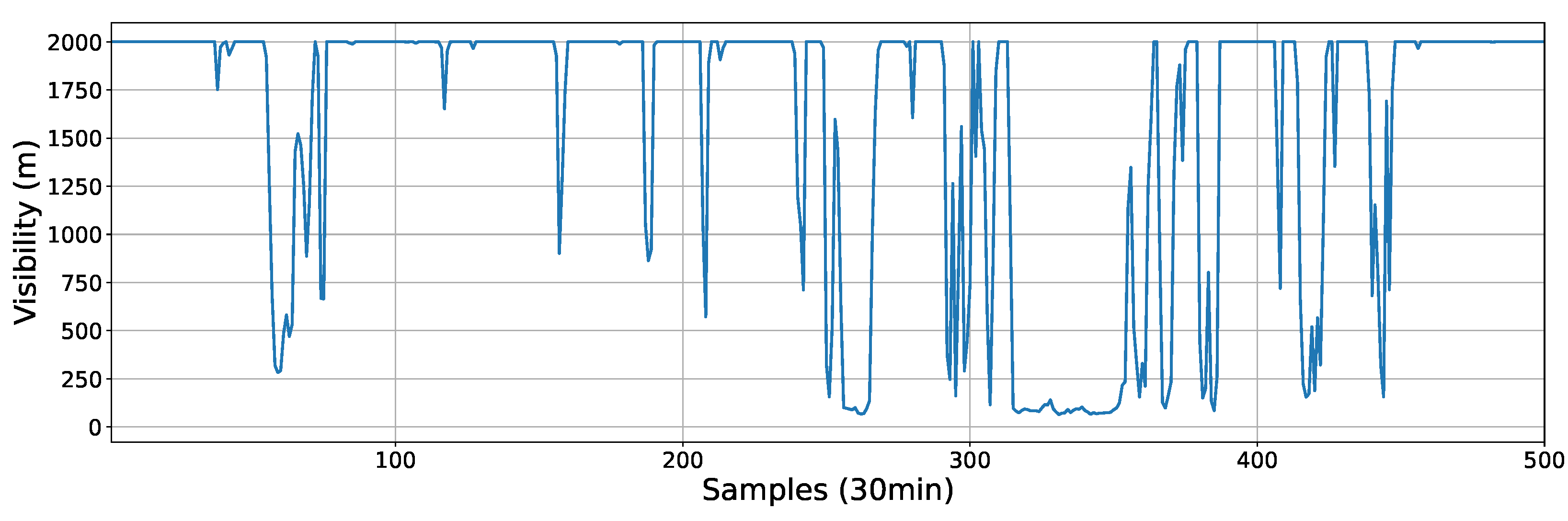
Visibility data measured at the Mondoñedo weather station, Galicia, Spain (43.38${}^{\circ }$ N, 7.37${}^{\circ }$ W), from 1 January 2018 to 30 November 2019 with a sampling frequency of 30 min were used in this paper, accounting for a total of 33,015 samples. This station measures visibility in the A8 motor-road in Lugo, where orographic (hill) fog usually occurs, forcing the closure of the motor-road in cases of extreme low-visibility events. Note that orographic fog is formed when moist air moves up a hill, resulting in expansion and cooling of the air to its dew point, and producing intense episodes of low visibility. The Mondoñedo area is known to experience frequent low-visibility events caused by orographic fog due to winds coming from the Cantabrian Sea.

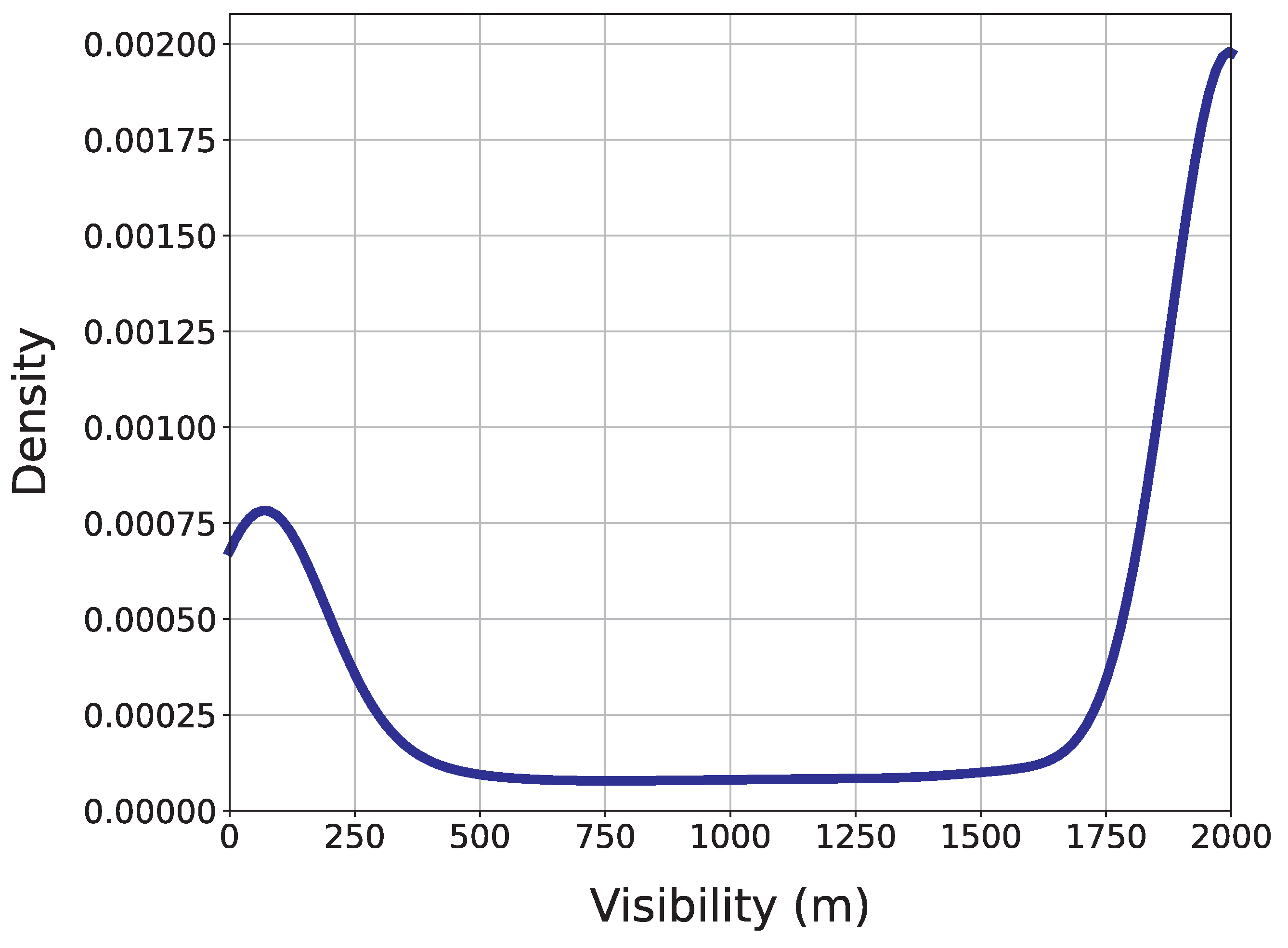
The data were acquired with a Biral WS-100 visibility sensor, which operates between 0 to 2000 m. The location of Mondoñedo is 140 m above sea level, and the distance to the sea is around 20 km; all the variables were acquired at 2 m height from the ground. Figure 5 illustrates the first 500 samples of the visibility time series, where the tendency of the data to remain close to 2000 or to 0 can be observed, while there are few data in intermediate ranges. This is further illustrated by plotting the density function of the data (Figure 6), where two peaks may be found: one near 0 m, corresponding to very low visibility levels, and a much more prominent peak near 2000 m, corresponding to events where visibility is very good.

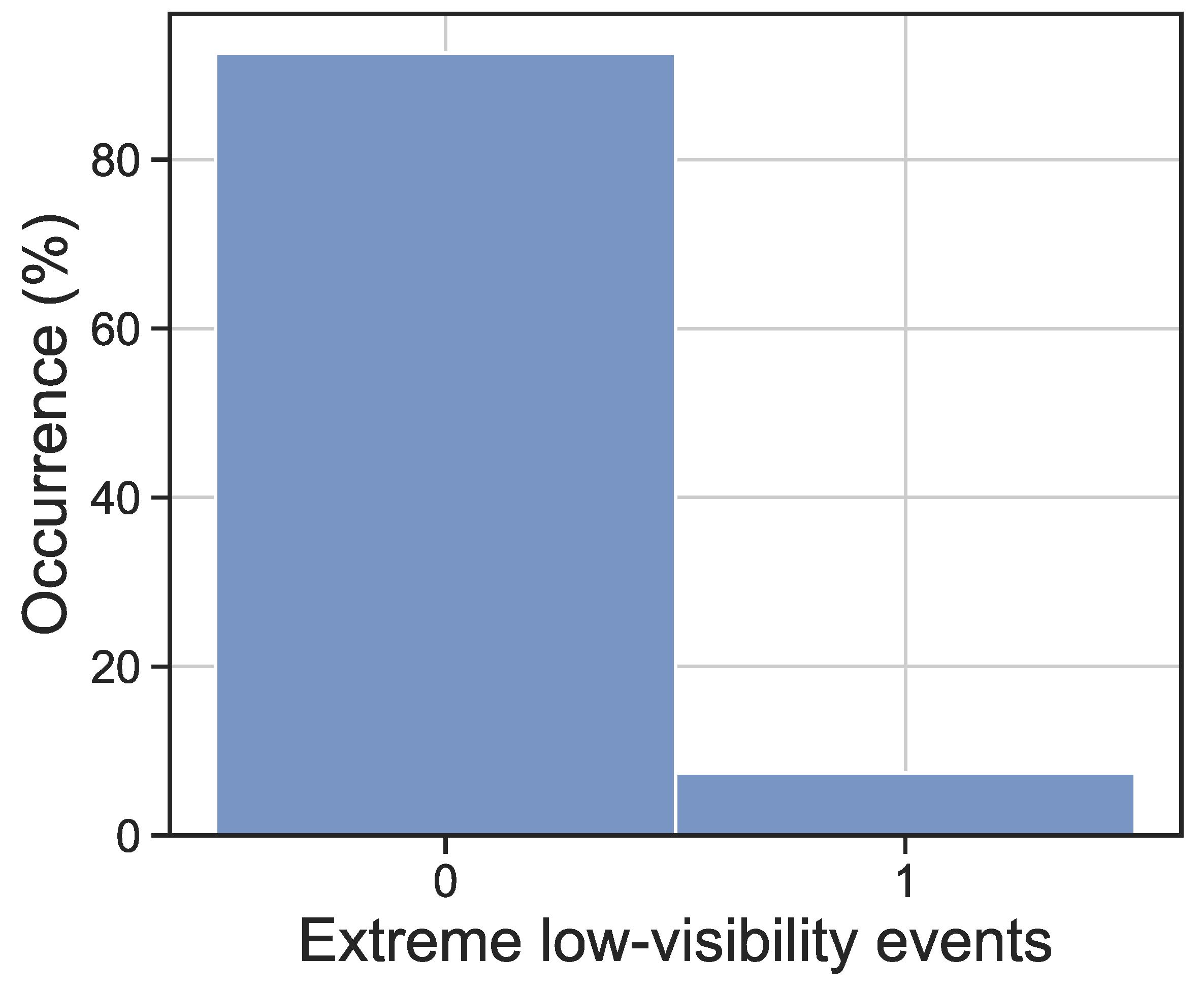
This work is focused on extreme low-visibility events, i.e., those fog events leading to visibility values below 40 m, which are those affecting the normal motor-road circulation the most. Since the problem is approached as a binary classification problem, Figure 7 shows the distribution of samples for each class, where extreme low-visibility events (class 1) account for 7.41% of the total number of samples. Thus, we focus on developing inductive and evolutionary rules for detecting and describing these specific events. The predictive variables used in this study for dealing with extreme low-visibility events consist of 11 exogenous meteorological variables registered by the same weather station at Mondoñedo (

Table 1. Predictive variables measured at Mondoñedo, Galicia, Spain.

Variable Name	Measured Variable
qpRa	Accumulated precipitation
at	Air temperature
ap	Atmospheric pressure
td	Dew temperature
st	Ground temperature
gr	Global solar radiation
hr	Relative humidity
sa	Salinity
wd	Wind direction
ws	Wind speed
vs	Visibility

). A brief discussion on the predictive variables is worthy here. Note that we used all the variables available (measured) in the Mondoñedo weather station; we did not carry out a previous step of feature selection, so we trust that the proposed algorithms are able to deal with possible redundancy between predicted variables, extracting the useful information from them in terms of their contribution to the visibility prediction. In addition, note that some of them are not related to visibility, but they are measured for other reasons, such as for the care of the road. For example, salinity of water in air is a variable related to corrosion of elements in the road, but it does not seem to be fully related to orographic fog. Similarly, accumulated precipitation (during the last hour) and ground temperature do not have much relation with the fog formation mechanism, but they can be involved in its persistence. The time horizons of the visibility forecast were established in +3 h, +5 h, and +10 h; therefore, measured variables acquired from $t=h$ (or ranging from $t=h-\mathrm{timestep}$ to $t=h$ in the case of DL methods) are used as predictors to forecast visibility at $t=h+3$, $t=h+5$, and $t=h+10$. 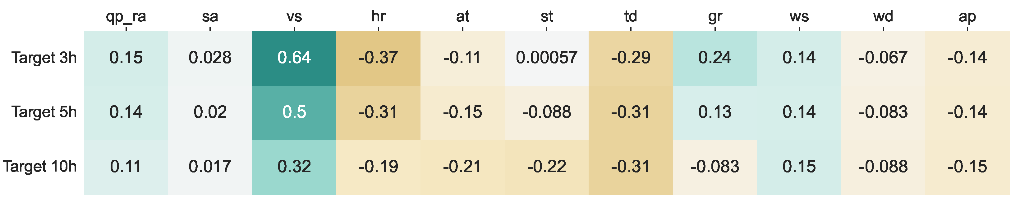In order to obtain an idea of the importance of the predictive variables, the Pearson correlation coefficient among the predictive variables and the target variable (prior to its binarization) is presented in Figure 8 for the three prediction time horizons considered. It can be seen how for some variables (qp_ra, sa, td, ws, ap) the correlation remains constant as the prediction horizon increases, while for others (vs, hr, at, st, gr, wd) the correlation varies. The variables showing the highest correlation are visibility in previous hours, the relative humidity, and the dew temperature. On the contrary, there are some other variables, such as salinity of water in air or ground temperature, which do not have, as expected, a high correlation with visibility prediction.

4. Experiments and Results

This section reports the results obtained in this work. In the first place, Section 4.2 analyzes the rules obtained by the induction and discovery algorithms. Next, Section 4.3 presents and discusses the results obtained for the first proposed methodology, consisting of the use of decision rules as a possible alternative to classification algorithms. Finally, results for the second approach are provided in Section 4.4, where information related to decision rules is incorporated into the ML/DL classifiers as an additional input feature.

4.1. Experimental Setup

The experimental setup, along with the parameters set for the different ML and DL methods, are detailed in this section. First, a preliminary dataset preparation is carried out. The steps of this preprocessing are: (1) Splitting the dataset into training and test (75–25%) subsets, ensuring that no test instance was seen by the classification methods during the training. Due to dealing with timed series data, instead of randomly splitting the datasets, the last 25% of the data were separated as test data. (2) Scaling of the features, which is important to ensure the upper and lower limits of data in the given predefined range. Feature standardization was performed, causing data to have zero mean and a unit variance (Equation (25)), where x is the original feature vector, $\overline{x}$ denotes the feature mean, and $\sigma$ its standard deviation.

$$x^{\prime }=\frac{x-\overline{x}}{\sigma }$$

(25)

Table 2. Experimental setup.

ML methods	SVC		RF
	regularization parameter	1	n estimators	400
	GNB		KNN
	variance smoothing	$1\times {10}^{-9}$	neighbors	20
	AB		GB
	estimators	50	estimators	100
			learning rate	1
			max depth	1
	MLP
	number of layers	1
	neurons per layer	500
	activation	relu
	solver	adam
	max epochs	300
DL methods	RNN		GRU
	number of layers	1	number of layers	1
	neurons per layer	64	neurons per layer	64
	loss	bin cross-entropy	loss	bin cross-entropy
	optimizer	adam	optimizer	adam
	batch size	32	batch size	32
	dense layers	2	batch size	2
	dense neurons	[64,1]	dense neurons	[64,1]
	activation	[relu,sigmoid]	activation	[relu,sigmoid]
	LSTM		CNN
	number of layers	1	number of CNN layers	2
	neurons per layer	64	filters	[32,32]
			kernel size	[3,23,1]
	loss	bin cross-entropy	loss	bin cross-entropy
	optimizer	adam	optimizer	adam
	batch size	32	batch size	32
	dense layers	2	batch size	3
	dense neurons	[64,1]	dense neurons	[64,32,1]
	activation	[relu,sigmoid]	activation	[relu,relu,sigmoid]
Rule learning	PRIM		DPCRO
	threshold	40	population size	125
	threshold type	<	$\rho$ initial occupation rate	0.6
	$\alpha$ for peeling	0.05	$F_b$ mutation probability	0.98
	$\alpha$ for pasting	0.01	$F_d$ depredation probability	0.2
	minimum support	0.04	$P_d$ depredation chosen rate	0.8
			number of attempt per larvae	3
			number of duplication allowed	6
			dynamic method	fitness
			dynamic metric	best
			amplification of probability	0.2
			operator 1	2Px
			operator 2	MPx
			operator 3	CS
			selected CS components	0.1
			operator 4	CM
			t scale of Cauchy	5
			operator 5	DE/rand/1
			F scale of DE	0.7
			$Cr$ selected DE components	0.8

shows the parameters used for the benchmark methods considered. All of the simulations were run on an Intel(R) Core(TM) i7-10700 CPU with 2.90 GHz and 16 GB RAM using the Python libraries sklearn, tensorflow, prim, and scipy.

In addition, we performed a previous optimization of the DPCRO-SL hyperparameters before using it for rule evolution. For this purpose, a genetic algorithm (GA) was used. There are many examples in the literature of successful uses of a GA for optimizing hyperparameters of, for example, neural networks [74]. That is why we opted for this option.

The search space includes several ranges for the hyperparameters values indicated in Table 2, and a list of possible operators for the DPCRO-SL. Specifically, this includes 2-point crossover (2Px), 3-point crossover (3Px), multipoint crossover (MPx), differential evolution DE/rand/1, differential evolution DE/best/1, component-wise swapping (CS), Gaussian mutation (GM), and Cauchy mutation (CM).

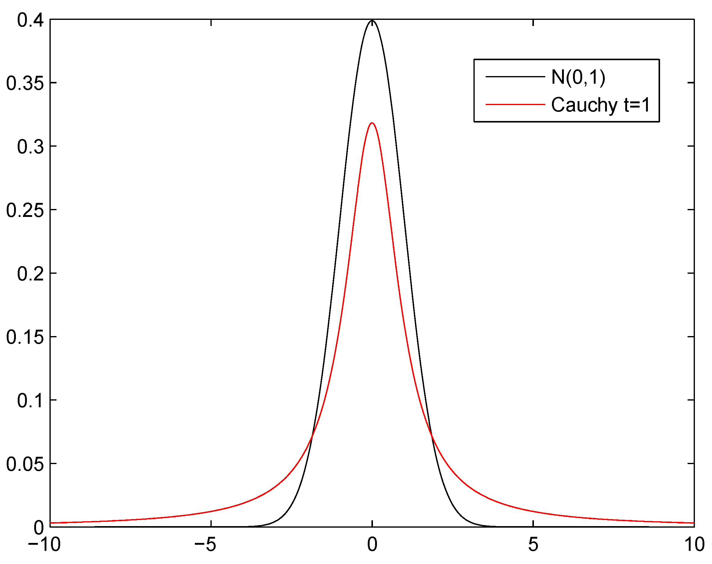
As a result of this process of optimization and selection of hyperparameters, we obtained the values specified in Table 2, as well as the operators defined in Section 2.1.2.3. It should be discussed why these operators perform better than others, i.e., DE/rand/1 instead of DE/best/1 and Cauchy mutation instead of Gaussian mutation. The reason in both cases is similar: the PRIM rules are already very good themselves, and we are unlikely to find an improvement in their neighborhood. Therefore, a mutation with greater variance such as the Cauchy (see Figure 2) facilitates a higher exploration than the Gaussian. Furthermore, DPCRO-SL itself is responsible for modifying the significance and quantity of the population with which each operator works at all times. This may explain why a 3Px crossover is not necessary. With 2Px already available to cross in blocks of components and MPx to cross several (or all) components, an intermediate operator between the two does not seem necessary, as the algorithm itself will combine MPx and 2Px to obtain the desired crossover. Eventually, the CS operator can offer a fine granularity level to modify the latest details close to the good solutions.

4.2. Analysis of the Extracted Decision Rules

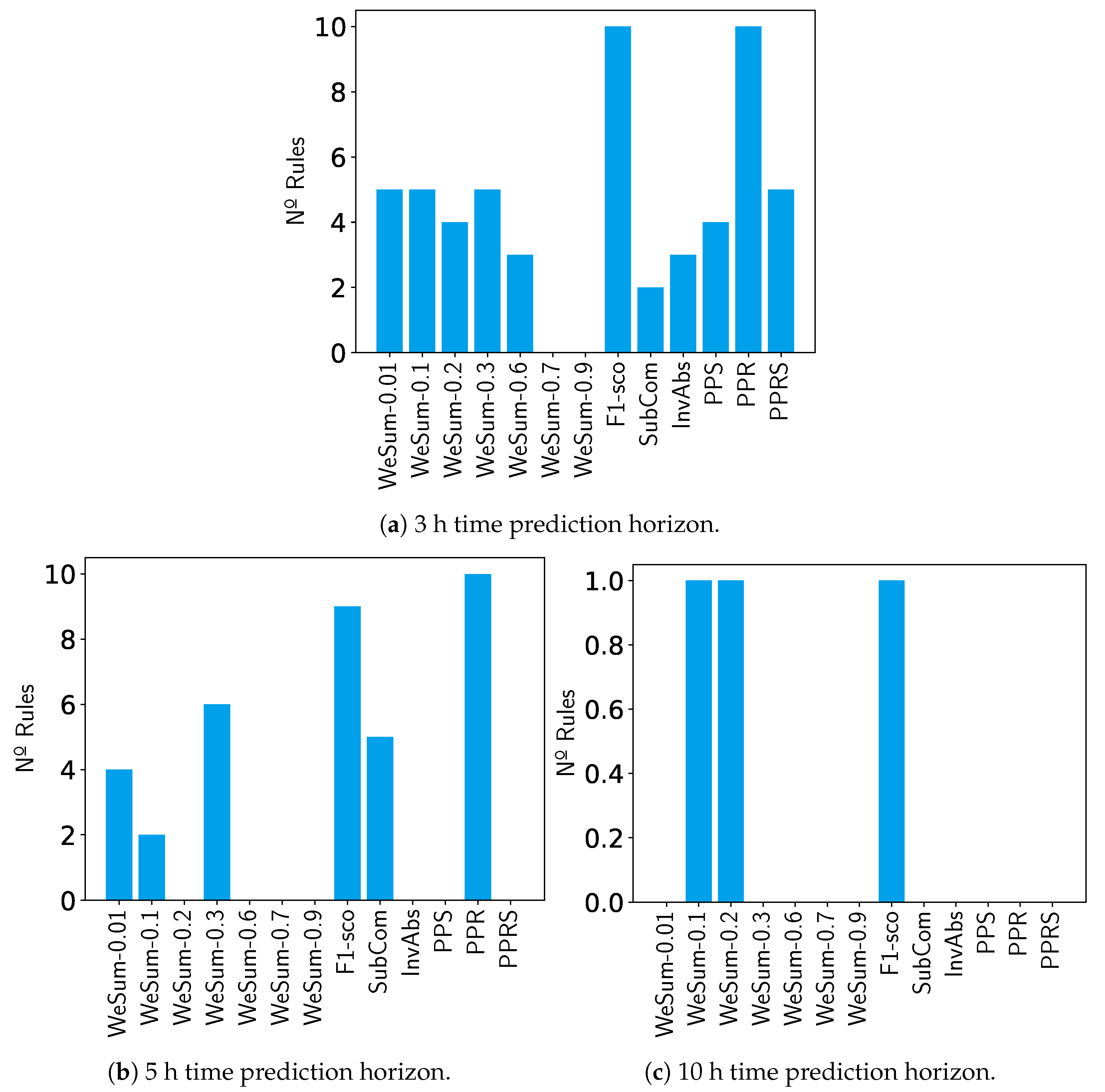
We start this section by analyzing the heuristics defined in Section 2.1.2.2. For the WeSum objective function, we set 0.01, 0.1, 0.2, 0.3, 0.6, 0.7, and 0.9 as values of $\alpha$. With this experiment, it is possible to verify whether it is better to penalize precision or support. Each heuristic is used 10 times to evolve and generate the best possible set of rules, i.e., 10 sets of rules (or boxes) are generated with each heuristic.

Then, we establish a threshold for minimum support size and precision for each box, namely, a minimum of 100 individuals (0.61% support) and a minimum of 40% precision. In this way we can measure how many boxes generated by each heuristic satisfy the threshold for each predictive horizon. Figure 9 shows the number of rule sets that fulfill the threshold on each time prediction horizon considered.

For the 3 h case (Figure 9a), the F1-score and PPR heuristics stand out from the others. As for WeSum, it seems that the low $\alpha$ values are better. Regarding the other heuristics, none of them can be said to work poorly for this time horizon, because they generate valid boxes. However, it can be seen that there are better heuristics within them.

In the 5 h horizon (Figure 9b), the heuristics F1-score and PPR continue to dominate, so that all (or almost all) the boxes generated outstrip the threshold. It also proves that WeSum is substantially better with small $\alpha$ values. Compared to other heuristics, only SubCom survives.

Finally, note that in the 10 h case (Figure 9c), only the F1-score and WeSum heuristics with small values of $\alpha$ fulfill the threshold.

With all these results in mind, we can draw several conclusions: first, we showed that alpha values between $[0.1,0.3]$ are the better option for WeSum heuristics. On the other hand, the best of all heuristics is undoubtedly F1-score. This is present in all time steps, producing very good sets of rules. It should also be mentioned that PPR performs well overall.

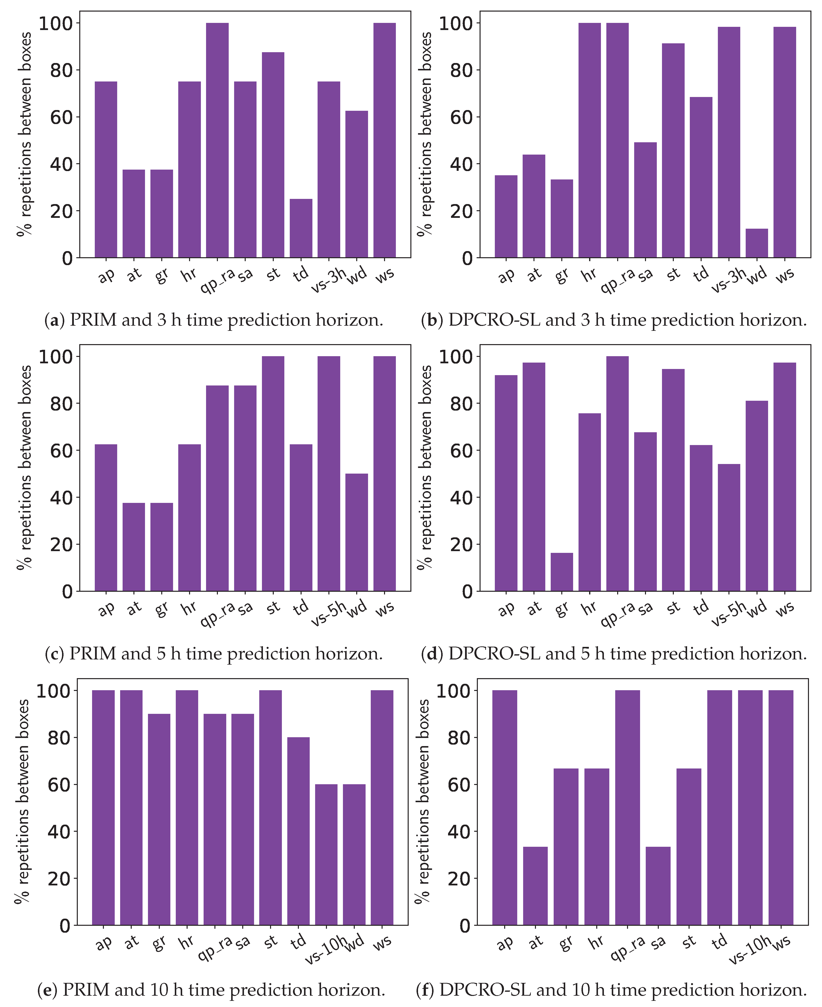
Afterwards, it is possible to observe in Figure 10 how many times each variable is repeated between the different boxes for each time horizon, both for the boxes of PRIM and those obtained by the DPCRO-SL. This helps us to analyze the importance of each variable over time, and the impact that each one of them can have on short- and long-term predictions. We consider the average behavior between PRIM and DPCRO-SL, remembering that the number of boxes that overtake the threshold is decreasing as the prediction horizon increases.

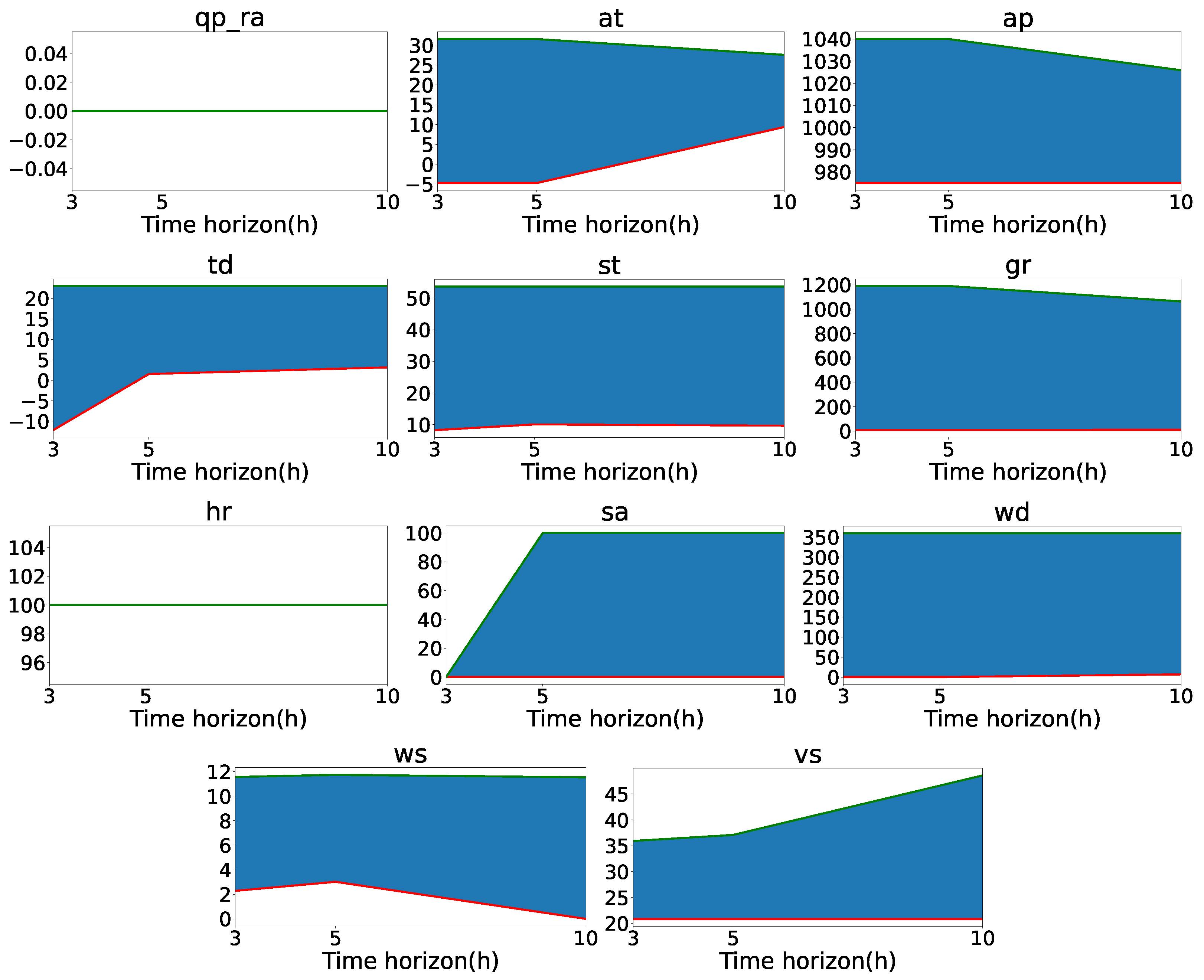
Instead, in Figure 11 we find the rules associated with each variable in the most restrictive box that was generated from each horizon. As mentioned in Section 2, these rules are expressed by a range of values to be taken by the variable, i.e., the lower limit (minimum) and upper limit (maximum) between which it has to be set. This means that if the range of values specified by the rules covers all possible values, the variable is not very important for the prediction; however, if the range is very small, the variable has great relevance. These figures allow us to reinforce the conclusions that can be obtained from the repetitions between boxes by time horizons.

The first variable to evaluate is atmospheric pressure. It is observed that with a forecast horizon of +3 h, this variable appears in approximately 75% of PRIM boxes and 35% of DPCRO-SL boxes. In the next horizon, it is present in 60% and 90% of the boxes, respectively. Finally, for the 10 h horizon, the atmospheric pressure is found in all generated boxes. The most restrictive box value ranges emphasizes this point, showing that for 3 h and 5 h, the atmospheric pressure is irrelevant, while for the 10 h case it has a more significant role. In summary, these results show that atmospheric pressure can have effects on extreme low-visibility events in the long-term.

Something similar happens with air temperature. For a time horizon of 3 h, it appears in 40% of PRIM boxes and 45% of DPCRO-SL boxes. For 5 h it is found at 40% and 95%, respectively, while for 10 h, it is found at 100% and 35%. Even more accentuated is the case of global solar radiation, with 40% and 35% for 3 h, 40% and 15% for 5 h, and 90% and 70% for 10 h. Figure 11 reinforces this because it is seen that for the most restrictive box, air temperature and global solar radiation acquire importance at 10h. This means that, similar to atmospheric pressure, air temperature and global solar radiation can influence the long-term prediction of the thick fog at Mondoñedo station.

Accumulated precipitation and relative humidity seem to be very important variables for the prediction, for the time prediction horizon of 3 h are found in 75% and 100% of PRIM boxes, respectively, and 100% of DPCRO-SL boxes in both cases. In the other horizons, they maintain a presence equal to or greater than 70% in the different boxes. The ranges of these variables for the most restrictive box are very small for all horizons. In particular, it is important for fog formation that the value of accumulated precipitation oscillates around 0 and the value of relative humidity is as close as possible to 100%.

Visibility and wind speed seem to be closely related. Both variables maintain a presence greater than 80% (and almost always close to or equal to 100%) in the boxes of PRIM and DPCRO-SL for all prediction time horizons, except for 10 h. In that case, the visibility is in 60% of the boxes. In the evolution of the value ranges we can see that both variables have a very considerable influence in the short and medium term, but not in the long-term prediction. Remembering that the 10 h horizon boxes are much less numerous, there is no contradiction in that the variables are in most 10 h boxes, as long as the rules associated with these variables select all (or almost all) the range of possible values.

Dew temperature is found in only 30% of PRIM boxes and 70% of DPCRO-SL boxes for 3 h. In 5 h and 10 h, their presence increases above 60% in all cases. This means that it is a variable whose influence is only appreciable in the medium–long term. The opposite is true of salinity. It is a variable that has a large presence in the boxes of 3 h (75% and 50%), but whose presence in 10 h is somewhat reduced, reaching 30% for DPCRO-SL. Since its range of values is increasing over time horizons, it is a variable with relevance only in the short-term prediction time horizon.

Finally, the variables floor temperature and wind direction are irrelevant in the prediction of thick fog, although for different reasons. The floor temperature is present in most boxes, both for PRIM and DPCRO-SL in different time steps. Its lowest presence is 60% in 10 h, remaining in other cases close to 90% or 100%. While this is true, Figure 11 shows us that rules associated with floor temperature, although always present, select the full (or nearly full) range of possible values. This can set a floor temperature minimum to 12, but with negligible importance. In the case of wind speed, even though we can see that the range of values always covers the totality, it is a variable that is not even present in most boxes. Except for the case of 80% in the boxes of DPCRO-SL in 5 h, in the other boxes, it is always below 60%, reaching 10% for DPCRO-SL in 3 h and 0% for DPCRO-SL in 5 h.

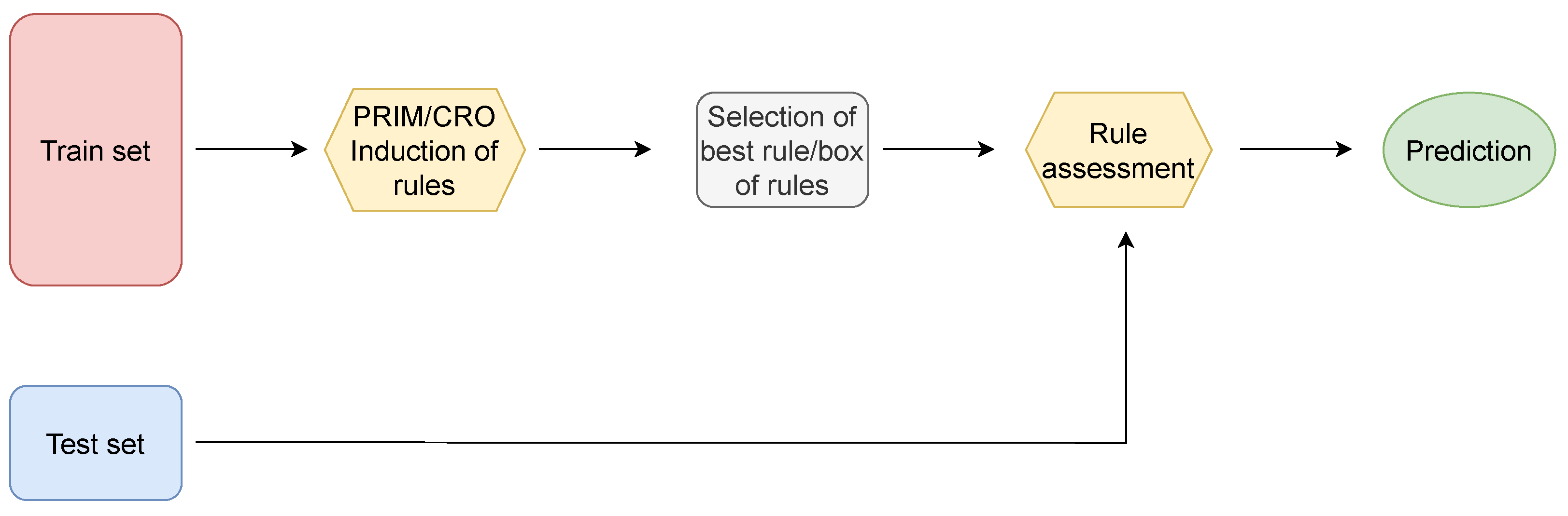
4.3. Use of Induced Rules to Anticipate the Presence of Thick Fog

Initially, the induced rules were used as a classification technique in order to anticipate the presence or absence of thick fog (Figure 12). For this purpose, two different approaches were tested. In the first one, given a test sample, each induced rule was assessed individually on the predictive variables and, if the rule was fulfilled, the prediction of that rule implied the presence of thick fog. Therefore, a different output was generated for each rule. In order to select the best performing rule, the performance of the forecasted values was also assessed individually on the training data, selecting the rules with the best scores for the three evaluated metrics, and computing those performances again on the test data.

The second approach consists of the evaluation of boxes of induced rules instead of just individual rules. Therefore, the outcome of the prediction for each box was considered to be positive (meaning that the presence of fog was forecasted) in the case that all the individual rules were fulfilled. Again, as the number of boxes is significant, the performance of each box is measured on train data, selecting the best performers for each metric and then assessing their values on the test data.

Test error metrics for these experiments are further displayed in Appendix A.

Table A1. Test results for all the classification methods evaluated, considering a time prediction horizon of +3 h.

		Recall	Precision	F1-Score
ML Classifiers	SVM	0.3859	0.6258	0.4774
	RF	0.5192	0.7500	0.6136
	GNB	0.9821	0.1793	0.3033
	KNN	0.3462	0.5305	0.4189
	AB	0.6103	0.6800	0.6432
	GB	0.6744	0.6518	0.6629
	MLP	0.3962	0.5776	0.4700
DL Classifiers	RNN	0.6218	0.5301	0.5723
	LSTM	0.6141	0.5275	0.5675
	GRU	0.5436	0.5443	0.5444
	CNN	0.6218	0.4821	0.5431
PRIM Boxes	Best Recall	0.8974	0.2965	0.4457
	Best Precision	0.3692	0.7291	0.4902
	Best F1	0.5115	0.5313	0.5212
CRO Boxes	Best Recall	0.8628	0.3441	0.4920
	Best Precision	0.0615	0.8727	0.1150
	Best F1	0.6346	0.5907	0.6119
PRIM Rules	Best Recall	1.0000	0.0945	0.1727
	Best Precision	0.4385	0.7185	0.5446
	Best F1	0.8064	0.5441	0.6498
CRO Rules	Best Recall	1.0000	0.0945	0.1727
	Best Precision	0.0692	0.8308	0.1278
	Best F1	0.7077	0.6359	0.6699

shows the test error metrics for the +3 h prediction time horizon of all the classifiers evaluated. Here, it can be seen how the GB is the most reliable ML method, remaining the most balanced performing method in the three metrics measured. Regarding the DL methods, the four classifiers yield similar performance, though slightly worse than the GB.

Moving on to the evaluation of rule boxes, it may be observed that, by prioritizing the recall metric among others, a superior result is obtained compared to the model with the highest recall of the benchmark methods, GNB, which obtains a 98% of detection of severe fog, albeit with a very low precision of 18%. Instead, the best PRIM box achieves a 90% of positive detection rate with a precision of almost 30%, and the best CRO box yields 86% of detection with a 34% of precision. When evaluating the more balanced boxes, the ones with better F1-score, it can be seen that, although they achieve quite good results, especially with the CRO-evolved boxes with a score of 0.61, they do not improve the results achieved by the GB (0.66).

Regarding the performance of the individual induced rules used as a classification method, it is observed that for both cases, PRIM and CRO-evolved rules, the ones with the higher recall values reach a 100% of thick fog detection rate, although the use of these rules as classifiers lacks practical interest due to the low accuracy rate achieved (9.45% for both cases). Nevertheless, the rules with the best F1-score present very competitive results for both cases, even surpassing the best ML classifier for the case of the CRO-evolved rule. Thus, the use of this rule constitutes a simpler, faster, and computationally cheaper alternative to the use of the ML/DL classification techniques.

Figure 13 displays the F1-score distribution for all the classification methods evaluated, showing a clear difference in error distribution shapes between the individual induced rules and the rule boxes: while the former reach higher maximum values than the latter, the average for the boxes remains higher. This is explained by the fact that boxes, as combinations of individual rules, take both strong and weak rules and combine them to produce more consistent results than the individual rules. However, in order to solve the prediction problem tackled in this paper, simply taking the best performing individual rule is more appealing, ensuring that it will lead to better results.

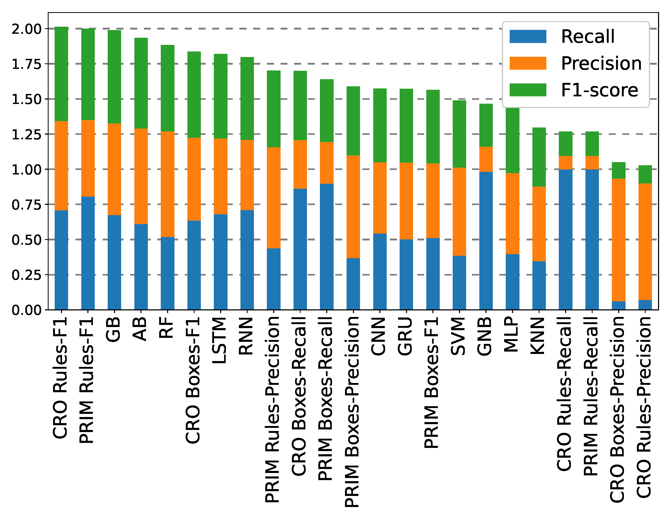
Finally, Figure 14 shows the comparison of all the classification methods tested in the +3 h prediction case, sorted from best to worst performance, and considering the sum of the three error metrics assessed. It is observed that the individual rules, both PRIM-induced and CRO-evolved, outperform the other methods used, representing the most optimal options for predicting thick fog events.

Regarding the performance of the employed methods for a 5 h prediction time horizon,

Table A2. Test results for all the classification methods evaluated, considering a time prediction horizon of +5 h.

		Recall	Precision	F1-Score
ML Classifiers	SVM	0.0718	0.5385	0.1267
	RF	0.2679	0.6786	0.3842
	GNB	0.9769	0.1414	0.2470
	KNN	0.2372	0.4960	0.3209
	AB	0.4269	0.6248	0.5072
	GB	0.6051	0.5438	0.5728
	MLP	0.3641	0.4855	0.4161
DL Classifiers	RNN	0.6154	0.4181	0.4979
	LSTM	0.5846	0.4101	0.4821
	GRU	0.3962	0.4491	0.4210
	CNN	0.6346	0.4267	0.5103
PRIM Boxes	Best Recall	0.7256	0.2432	0.3643
	Best Precision	0.3333	0.5977	0.4280
	Best F1	0.3333	0.5977	0.4280
CRO Boxes	Best Recall	0.7231	0.2554	0.3775
	Best Precision	0.0256	0.4082	0.0483
	Best F1	0.6885	0.3563	0.4696
PRIM Rules	Best Recall	1.0000	0.0945	0.1727
	Best Precision	0.4295	0.5971	0.4996
	Best F1	0.4295	0.5971	0.4996
CRO Rules	Best Recall	1.0000	0.0945	0.1727
	Best Precision	0.2615	0.6602	0.3747
	Best F1	0.7372	0.4733	0.5764

shows the error metrics for each of the classification techniques. Here, it can be noted how the previously drawn conclusions for the preceding time horizon are maintained. GB remains as the ML/DL method with the best F1-score, but this result is surpassed by the best individual rule evolved with CRO. Regarding the rule boxes, it is shown how in terms of F1-score neither PRIM nor CRO boxes outperform the best individual rules, with detection rates of above 72% with precision around 25%.

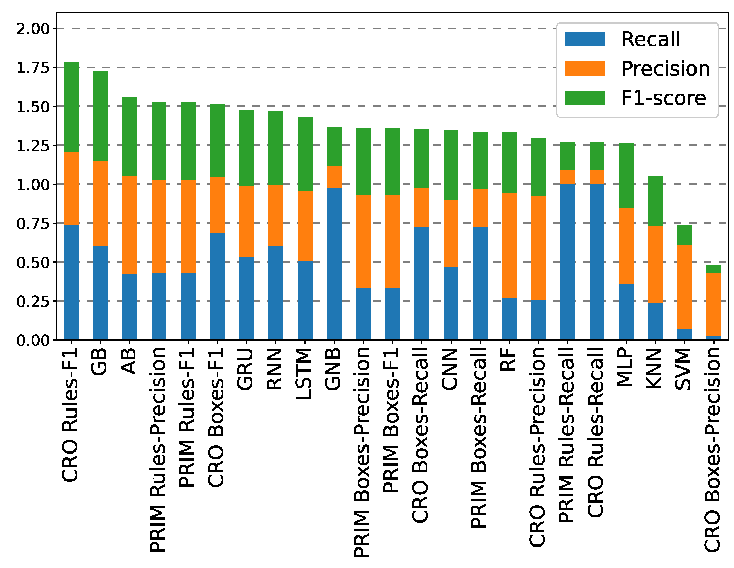
Figure 15 shows the sorted comparison of the methods’ performances, headed by the best (in terms of F1-score) individual rule evolved by CRO. Then, the two boosting ML methods, GB and AB, are the next-best performers, followed by the individual rules induced by PRIM.

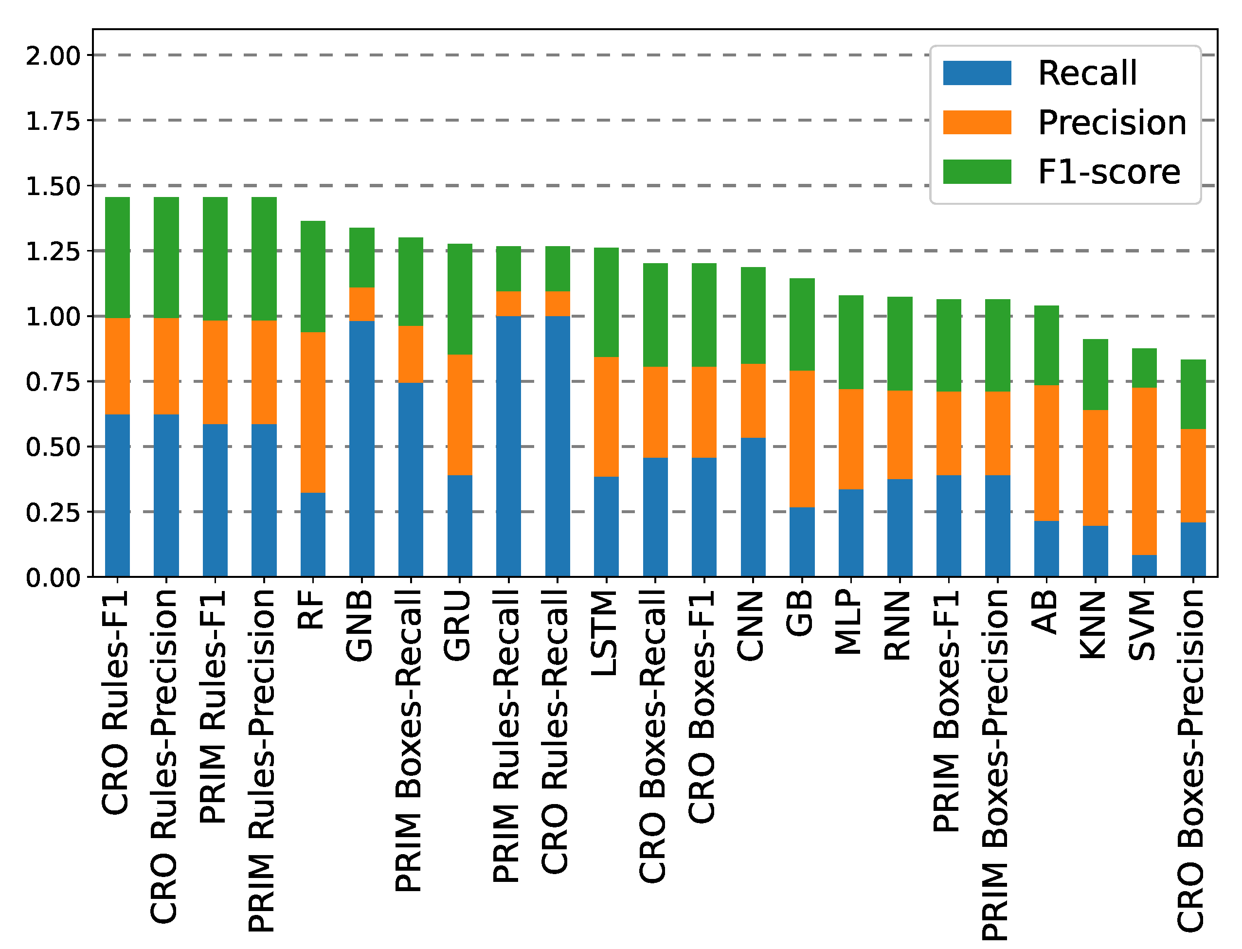
Finally,

Table A3. Test results for all the classification methods evaluated, considering a time prediction horizon of +10 h.

		Recall	Precision	F1-Score
ML Classifiers	SVM	0.0846	0.6408	0.1495
	RF	0.3231	0.6161	0.4239
	GNB	0.9808	0.1293	0.2285
	KNN	0.1962	0.4435	0.2720
	AB	0.2154	0.5201	0.3046
	GB	0.2667	0.5239	0.3534
	MLP	0.3372	0.3828	0.3586
DL Classifiers	RNN	0.5910	0.3574	0.4454
	LSTM	0.4064	0.4440	0.4244
	GRU	0.4179	0.3638	0.3890
	CNN	0.4654	0.3845	0.4211
PRIM Boxes	Best Recall	0.7449	0.2177	0.3369
	Best Precision	0.3897	0.3217	0.3525
	Best F1	0.3897	0.3217	0.3525
CRO Boxes	Best Recall	0.4577	0.3480	0.3953
	Best Precision	0.2103	0.3581	0.2649
	Best F1	0.4577	0.3480	0.3953
PRIM Rules	Best Recall	1.0000	0.0946	0.1728
	Best Precision	0.5872	0.3955	0.4727
	Best F1	0.5872	0.3955	0.4727
CRO Rules	Best Recall	1.0000	0.0946	0.1728
	Best Precision	0.6244	0.3681	0.4631
	Best F1	0.6244	0.3681	0.4631

displays the test results for the time prediction horizon at +10 h. In this case, the conclusions drawn are slightly different from the previous scenarios: first, RF becomes the best performing ML classifier instead of GB. Moreover, DL methods outperform ML models in this long-term prediction, with the RNN model being the one with the higher F1-score. Differences are also observed in the performance analysis of the individual rules, where, in this case, it is the PRIM-induced rules that offer the best overall performance in terms of F1-score, with a significant increase of 6% with respect to the best ML/DL model.

Figure 16 shows the test performance of all the methods sorted according to the sum of the three error metrics assessed. In this case, both the CRO-evolved and the PRIM-induced individual rules remain as the most reliable and robust classifiers, outperforming the ML/DL models.

4.4. Use of Rules as Additional Predictive Variables in ML/DL

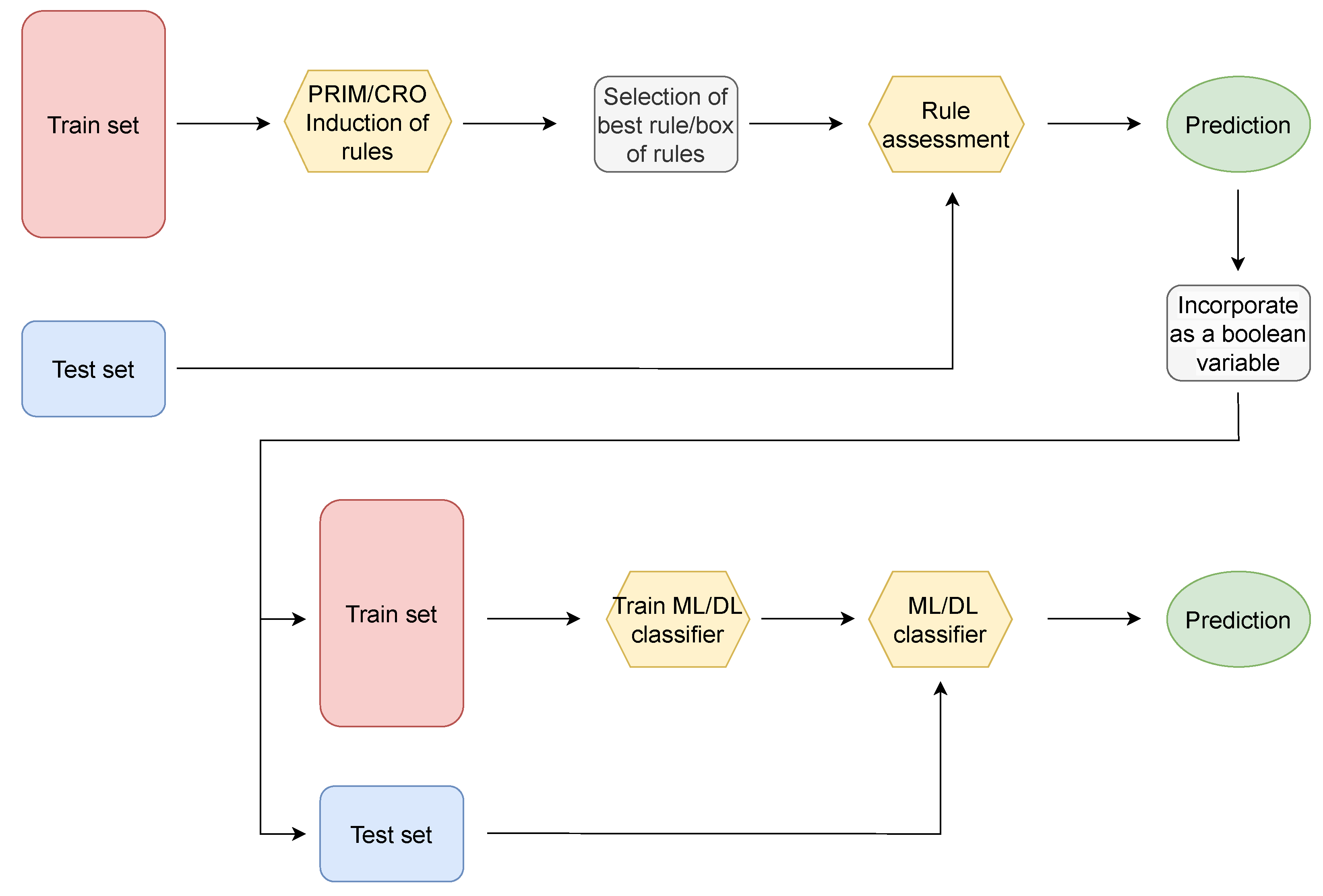
The second methodology implemented in this paper involves the use of the induced rules as an additional predictive Boolean variable in the ML/DL classification models. In this way, once the inducted rules have been assessed both on the train and test samples, a Boolean variable is created according to whether the rule (or box of rules) is fulfilled or not. This additional variable is then inserted in addition to the meteorological variables that form the train and test data. Subsequently, the ML and DL classification models are trained using the new training set, and their test predictions are further evaluated. Figure 17 illustrates the flow diagram of the followed methodology.

Five different strategies were studied for selecting the additional variables to be introduced into the system, which are shown in

Table 3. Different scenarios evaluated when introducing the rule-related information into the database.

Case 0	Original training data.
Case 1	Addition of PRIM-induced box with highest F1-score on training data.
Case 2	Addition of CRO-evolved box with highest F1-score on training data.
Case 3	Addition of PRIM-induced rule with highest F1-score on training data.
Case 4	Addition of CRO-evolved rule with highest F1-score on training data.
Case 5	cAddition of four previous mentioned variables.

. The first and second cases consist of the selection of the best box of rules, corresponding with the one presenting the highest F1-score in the training data, both the PRIM-induced best box (Case 1) and the CRO-evolved best box (Case 2). The same approach was repeated using the best individual rules instead of sets of rules in Cases 3 (best rule induced by PRIM) and 4 (best CRO-evolved rule). Finally, Case 5 adds the four preceding cases’ variables to the database.

Next, the results obtained for the three prediction time horizons evaluated (+3 h,+5 h, and +10 h) are presented and discussed. Test error metrics for these experiments are further displayed in Appendix B. 

Table A4. Test results for induced/evolved rules used as an additional predictive feature, considering a time prediction horizon of +3 h.

		SVC			RF			GNB			KNN
		Rec	Prec	F-1	Rec	Prec	F1	Rec	Prec	F1	Rec	Prec	F1
Case 0		0.39	0.63	0.48	0.52	0.75	0.48	0.98	0.18	0.30	0.35	0.53	0.42
Case 1		0.53	0.63	0.58	0.51	0.76	0.61	0.98	0.18	0.31	0.39	0.58	0.47
Case 2		0.63	0.59	0.61	0.50	0.75	0.60	0.98	0.18	0.31	0.50	0.66	0.57
Case 3		0.72	0.65	0.69	0.52	0.75	0.62	0.98	0.19	0.32	0.46	0.66	0.54
Case 4		0.71	0.64	0.67	0.51	0.74	0.61	0.98	0.19	0.31	0.54	0.70	0.61
Case 5		0.71	0.64	0.67	0.53	0.75	0.62	0.98	0.22	0.36	0.59	0.71	0.64
		AB			GB			MLP			RNN
		Rec	Prec	F1	Rec	Prec	F1	Rec	Prec	F1	Rec	Prec	F1
Case 0		0.61	0.68	0.64	0.67	0.65	0.66	0.40	0.58	0.47	0.62	0.53	0.57
Case 1		0.61	0.68	0.64	0.67	0.65	0.66	0.50	0.55	0.52	0.64	0.51	0.57
Case 2		0.61	0.68	0.64	0.67	0.65	0.66	0.56	0.59	0.58	0.63	0.53	0.58
Case 3		0.61	0.68	0.64	0.67	0.65	0.66	0.53	0.58	0.55	0.77	0.54	0.64
Case 4		0.61	0.68	0.64	0.67	0.65	0.66	0.65	0.63	0.64	0.83	0.49	0.61
Case 5		0.61	0.68	0.64	0.67	0.65	0.66	0.60	0.67	0.63	0.75	0.57	0.65
		LSTM			GRU			CNN			Average
		Rec	Prec	F1	Rec	Prec	F1	Rec	Prec	F1	Rec	Prec	F1
Case 0		0.61	0.53	0.57	0.54	0.54	0.54	0.62	0.48	0.54	0.57	0.55	0.53
Case 1		0.60	0.58	0.59	0.59	0.57	0.58	0.59	0.48	0.53	0.60	0.56	0.55
Case 2		0.50	0.53	0.51	0.47	0.56	0.51	0.67	0.46	0.54	0.61	0.56	0.56
Case 3		0.70	0.62	0.66	0.63	0.54	0.58	0.52	0.55	0.53	0.65	0.58	0.58
Case 4		0.70	0.64	0.67	0.50	0.56	0.53	0.58	0.55	0.56	0.66	0.59	0.59
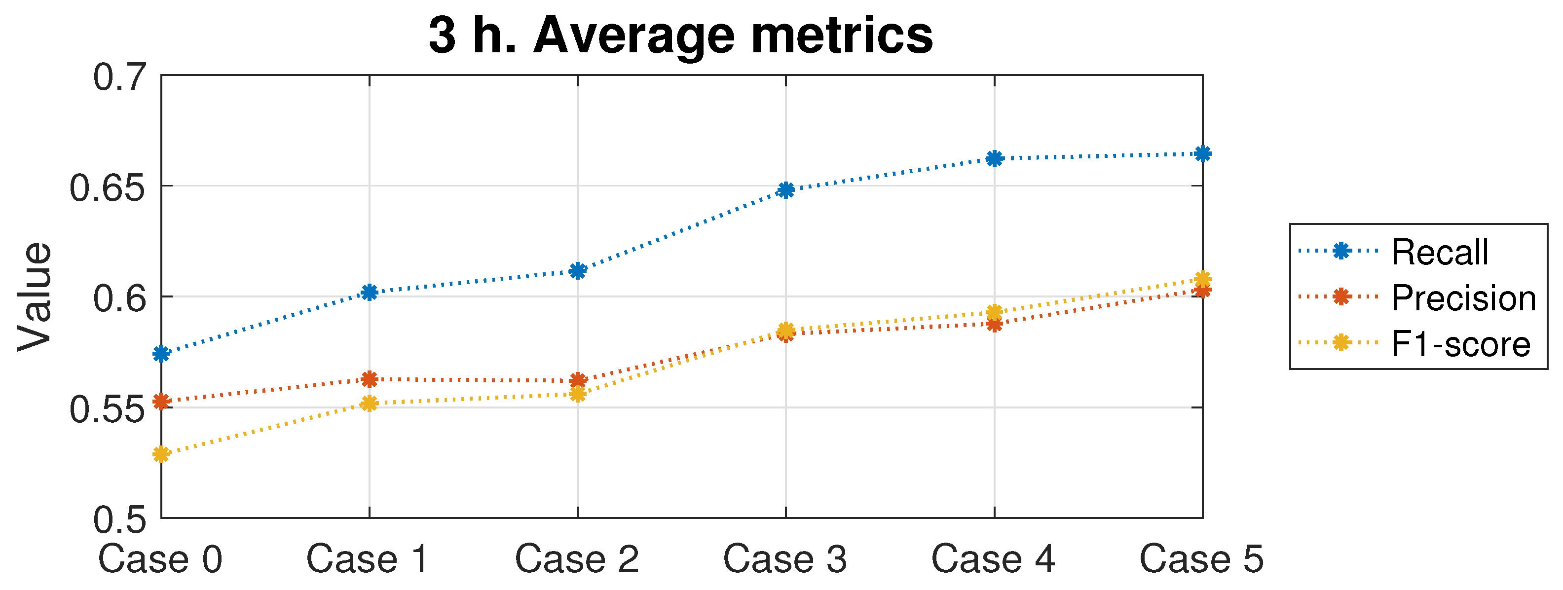
Case 5		0.67	0.65	0.66	0.64	0.55	0.59	0.57	0.54	0.56	0.66	0.60	0.61

displays the results for the +3 h prediction, revealing the substantial improvement in the three evaluated error metrics compared tothe classifiers experiment when introducing as predictive variables the information related to the different rules or sets of rules, both induced and evolved. It is noteworthy that the only models that maintain identical results are those with a boosting architecture (AB and GB), and it becomes apparent that the added variables do not contribute towards the ensembles that form these methods.

When comparing the different cases studied regarding which rules are introduced as additional variables, by observing the average of the error metrics from all classifiers, it can be noticed that Case 5 (which includes the four variables studied) is the one that achieves better results, improving the recall metric by 15.8% over the initial results, the precision by 9.1%, and the F1-score by 15.10%. For the sake of clarity, the average metrics of all classifiers for the six cases evaluated are represented in Figure 18. Three conclusions can be drawn from this Figure: (1) the best performing case is clearly Case 5, the one adding the four additional variables into the system, meaning that the models perform better when handling all the possible information they can have; (2) Case 2 performs better than Case 1, and Case 4 performs better than Case 3, indicating that in both situations, whether dealing with individual rules or with sets of rules, it yields better results to work with CRO-evolved rules than with those induced by PRIM; and (3) Cases 3 and 4 perform far better than Cases 1 and 2, suggesting that dealing with a single rule is more efficient than working with a complete set of rules.

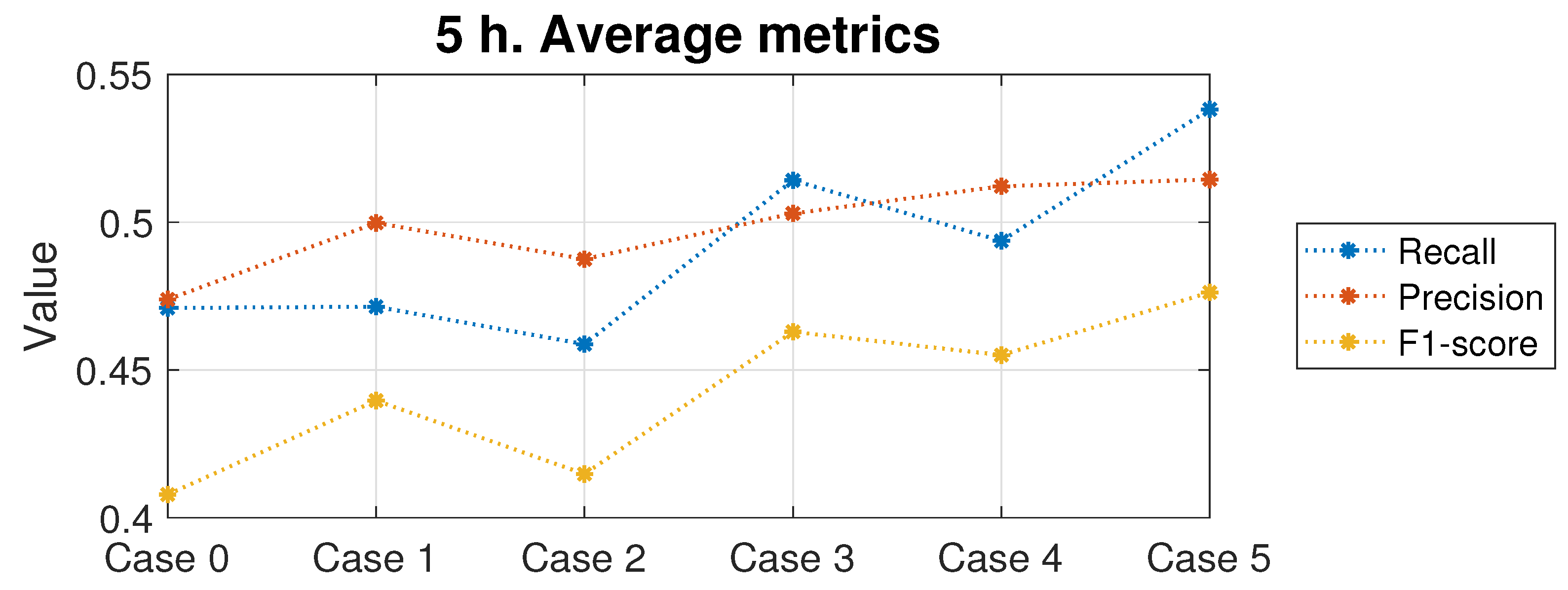
Subsequently, results for the 5 h time prediction horizon are shown in

Table A5. Test results for induced/evolved rules used as an additional predictive feature, considering a time prediction horizon of +5 h.

		SVC			RF			GNB			KNN
		Rec	Prec	F-1	Rec	Prec	F1	Rec	Prec	F1	Rec	Prec	F1
Case 0		0.07	0.54	0.13	0.27	0.68	0.38	0.98	0.14	0.25	0.24	0.50	0.32
Case 1		0.33	0.60	0.43	0.29	0.68	0.41	0.98	0.15	0.25	0.27	0.57	0.36
Case 2		0.13	0.63	0.21	0.27	0.66	0.38	0.98	0.14	0.25	0.27	0.54	0.36
Case 3		0.43	0.60	0.50	0.29	0.65	0.40	0.99	0.15	0.26	0.30	0.62	0.40
Case 4		0.37	0.65	0.47	0.27	0.64	0.38	0.99	0.15	0.25	0.31	0.64	0.42
Case 5		0.42	0.63	0.50	0.27	0.66	0.39	0.98	0.16	0.28	0.29	0.64	0.40
		AB			GB			MLP			RNN
		Rec	Prec	F1	Rec	Prec	F1	Rec	Prec	F1	Rec	Prec	F1
Case 0		0.43	0.62	0.51	0.61	0.54	0.57	0.36	0.49	0.42	0.62	0.42	0.50
Case 1		0.43	0.62	0.51	0.61	0.54	0.57	0.41	0.48	0.44	0.53	0.45	0.49
Case 2		0.43	0.62	0.51	0.61	0.54	0.57	0.38	0.49	0.43	0.55	0.43	0.49
Case 3		0.43	0.62	0.51	0.61	0.54	0.57	0.44	0.50	0.47	0.61	0.46	0.53
Case 4		0.43	0.62	0.51	0.61	0.54	0.57	0.44	0.50	0.47	0.66	0.44	0.53
Case 5		0.43	0.62	0.51	0.61	0.54	0.57	0.48	0.53	0.50	0.68	0.48	0.56
		LSTM			GRU			CNN			Average
		Rec	Prec	F1	Rec	Prec	F1	Rec	Prec	F1	Rec	Prec	F1
Case 0		0.58	0.41	0.48	0.40	0.45	0.42	0.63	0.43	0.51	0.47	0.47	0.41
Case 1		0.46	0.51	0.48	0.49	0.49	0.49	0.39	0.41	0.40	0.47	0.50	0.44
Case 2		0.48	0.52	0.50	0.51	0.44	0.47	0.44	0.35	0.39	0.46	0.49	0.41
Case 3		0.45	0.47	0.46	0.49	0.45	0.47	0.63	0.46	0.53	0.51	0.50	0.46
Case 4		0.57	0.53	0.55	0.53	0.47	0.45	0.36	0.44	0.39	0.49	0.51	0.46
Case 5		0.41	0.46	0.43	0.60	0.51	0.55	0.75	0.41	0.53	0.54	0.51	0.48

and Figure 19. Again, a substantial improvement is observed in the performance of all the classification methods, except for the boosting methods, when adding the induced/evolved rules and boxes of rules as additional predictive features. Specifically, the average improvement shown by these models is 14.9% for the recall metric, 8.5% for the precision, and 17.1% for the F1-score, considering the best performing way of inputting the rule-based information into the systems: adding to the original database the four extra variables (Case 5). Figure 19 illustrates the differences between the distinct cases evaluated. On this occasion, it is worth mentioning that the use of PRIM-induced rules and rule boxes (Cases 1 and 3) performs better than those evolved with CRO (Cases 2 and 4). However, undoubtedly, the best performing approach continues to be Case 5, with an important enhancement of the three error metrics considered.

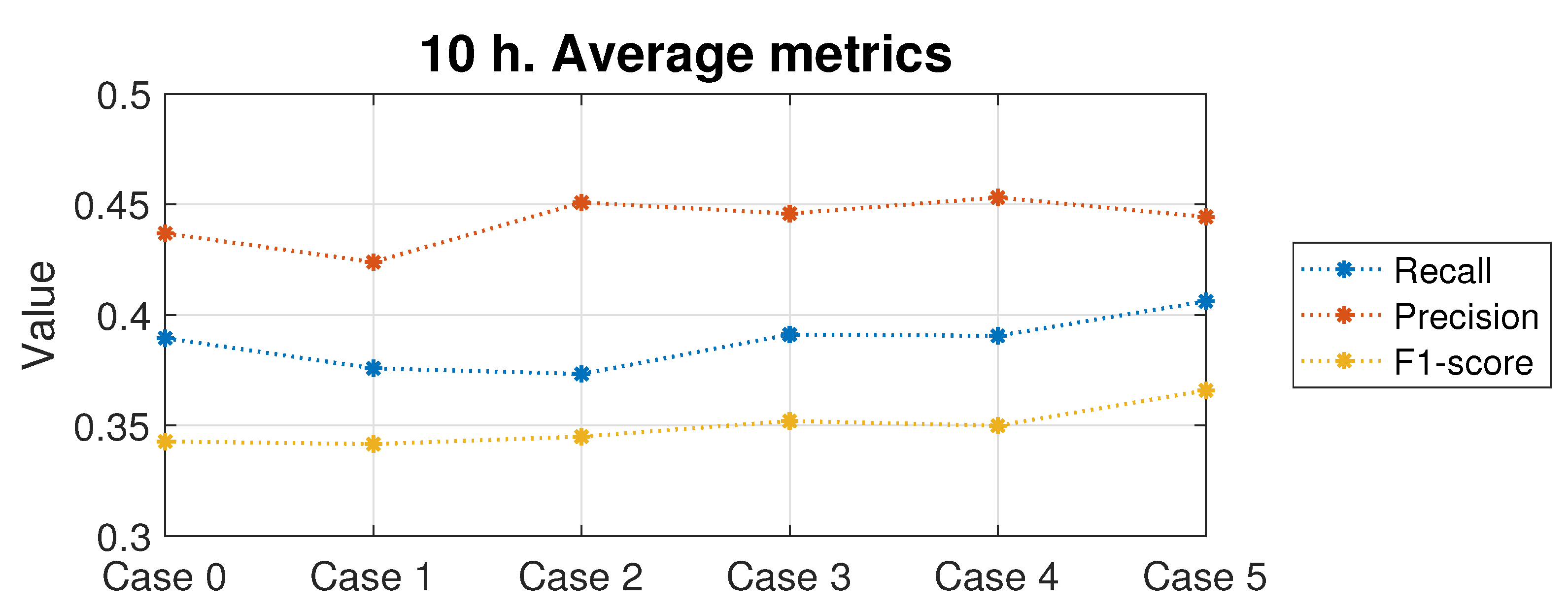
Finally,

Table A6. Test results for induced/evolved rules used as an additional predictive feature, considering a time prediction horizon of +10 h.

		SVC			RF			GNB			KNN
		Rec	Prec	F-1	Rec	Prec	F1	Rec	Prec	F1	Rec	Prec	F1
Case 0		0.08	0.64	0.15	0.32	0.62	0.42	0.98	0.13	0.23	0.20	0.44	0.27
Case 1		0.16	0.49	0.25	0.27	0.60	0.38	0.98	0.13	0.23	0.22	0.49	0.30
Case 2		0.11	0.62	0.18	0.27	0.61	0.38	0.98	0.13	0.23	0.22	0.50	0.30
Case 3		0.12	0.61	0.20	0.31	0.61	0.41	0.98	0.13	0.23	0.22	0.52	0.31
Case 4		0.11	0.61	0.19	0.31	0.64	0.42	0.98	0.13	0.23	0.22	0.49	0.30
Case 5		0.19	0.51	0.28	0.30	0.58	0.39	0.98	0.14	0.24	0.25	0.49	0.33
		AB			GB			MLP			RNN
		Rec	Prec	F1	Rec	Prec	F1	Rec	Prec	F1	Rec	Prec	F1
Case 0		0.22	0.52	0.30	0.27	0.52	0.35	0.34	0.38	0.36	0.59	0.36	0.45
Case 1		0.22	0.52	0.30	0.24	0.51	0.33	0.41	0.40	0.41	0.41	0.37	0.39
Case 2		0.22	0.52	0.30	0.24	0.51	0.33	0.44	0.42	0.43	0.43	0.39	0.41
Case 3		0.22	0.52	0.30	0.27	0.52	0.35	0.48	0.43	0.45	0.55	0.34	0.42
Case 4		0.22	0.52	0.30	0.27	0.52	0.35	0.29	0.50	0.37	0.59	0.37	0.46
Case 5		0.22	0.52	0.30	0.23	0.50	0.31	0.41	0.50	0.45	0.57	0.37	0.44
		LSTM			GRU			CNN			Average
		Rec	Prec	F1	Rec	Prec	F1	Rec	Prec	F1	Rec	Prec	F1
Case 0		0.41	0.44	0.42	0.42	0.36	0.39	0.47	0.38	0.42	0.39	0.44	0.34
Case 1		0.39	0.39	0.39	0.38	0.41	0.39	0.45	0.35	0.39	0.38	0.42	0.34
Case 2		0.40	0.45	0.42	0.40	0.43	0.41	0.40	0.39	0.39	0.37	0.45	0.35
Case 3		0.42	0.44	0.43	0.34	0.44	0.38	0.39	0.35	0.37	0.39	0.45	0.35
Case 4		0.39	0.49	0.43	0.35	0.36	0.36	0.56	0.35	0.44	0.39	0.45	0.35
Case 5		0.37	0.49	0.42	0.42	0.42	0.42	0.50	0.38	0.43	0.40	0.44	0.37

displays the results for the 10-hour-ahead forecasting. In this case, with the exception of the SVC and KNN models, it can be observed how the improvements achieved are smaller than in the previous time horizons. Again, the best performing scenario is Case 5, providing an average improvement of 2.6% in the recall metric, keeping the same precision values and improving the F1-score by 8.8%. Figure 20 illustrates how, in this long-term prediction case, Cases 1 to 4 exhibit very similar performances to the initial database. Only in Case 5, when adding all the supplementary variables to the database, are the recall and F1-score increased, though without any improvement in the precision metric.

5. Conclusions

In this paper, the prediction of extreme low-visibility events due to orographic fog at the A-8 motor-road (Galicia, Northern Spain) was tackled as a binary classification problem for three different prediction time horizons, covering from mid-term to long-term prediction problems (+3, +5, and +10 h). Specifically, the approach pursued in this work focused on the use of explainable classification models based on inductive and evolutionary decision rules. This approach eases the interpretation of the results, thus providing an understanding of the model mechanisms and of the reason why the predictions are obtained. This provides a critical piece of information that is especially relevant in challenging forecasting problems such as long-term predictions (10 h) of extreme low-visibility events, where the low persistence of fog significantly hinders the predictions. In these cases, having a physical explainability of the forecasts can help a committee of experts in decision making at an early stage.

As a preliminary step, a detailed analysis of the rules and sets of rules extracted by the PRIM and CRO algorithms was conducted, concluding that (1) accumulated precipitation and relative humidity are found to be the most important variables, consistently keeping their significance throughout the different time forecasting horizons evaluated; (2) visibility, wind speed, and salinity present a strong influence over the short- and medium-term forecast, but lose relevance in the long term; (3) regarding the medium- and long-term forecasting, the main significant variables arerelated to atmospheric pressure, air temperature, global solar radiation, and dew temperature; and (4) some variables, such as floor temperature and wind direction, are found to remain irrelevant and of no interest for the prediction of thick fog across the different prediction horizons.

The first evaluated methodology consisted of applying PRIM-induced and CRO-evolved rules as a possible simpler alternative to more complex ML/DL classification methods, with a reasonable performance in this particular case. Specifically, a comparison among different strategies of rules-based information application to forecast the presence or absence of thick fog was carried out, demonstrating some performance advantages of these rule-based strategies over conventional ML/DL classifiers, with slight improvements over the best classification model of 1.05% for the 3 h time horizon, 0.63% for the 5 h, and 6.13% for the 10 h (on the F1-score metric). These methods also offer a further strength over the ML/DL models, i.e., their complexity, computational costs, and training time are substantially lower, as they are far simpler models.

The second proposed strategy tested consists of the integration of the information provided by the induced/evolved rules in the ML/DL techniques, as additional predictive features, in order to enrich the complex ML/DL models. Different scenarios were tested to assess the most appropriate way to incorporate the rule-based information into the classification systems. This approach led to a significant enhancement of the classification models’ performances for the three prediction time horizons assessed, and the achieved F1-score improvement ratios attained values of 15.10% for the 3 h time horizon, 17.10% for the 5 h, and 8.80% for the 10 h.

In this work we showed how the use of explainable induced and evolved rules can be of significant interest in the prediction of extreme low-visibility events, providing strong results for complex forecasting problems such as long-term prediction. Note that the proposal in this paper is generalizable to any other location where orographic fog occurs. Future lines of research will consist of improving the way in which rule information is utilized for prediction, by implementing ensembles of rules or rule boxes with a higher level of complexity, combining the individual rules into a fuzzy-based controller to refine the final results obtained, or testing functional regression methods as final outcomes for the system.

References

1. Cho, H.J.; Kim, K.S. Development of hazardous road fog index and its application. J. East. Asia Soc. Transp. Stud. 2005, 6, 3357–3371. [Google Scholar]
2. Peng, Y.; Abdel-Aty, M.; Lee, J.; Zou, Y. Analysis of the impact of fog-related reduced visibility on traffic parameters. J. Transp. Eng. Part A Syst. 2018, 144, 04017077. [Google Scholar] [CrossRef]
3. Román-Cascón, C.; Steeneveld, G.; Yagüe, C.; Sastre, M.; Arrillaga, J.; Maqueda, G. Forecasting radiation fog at climatologically contrasting sites: Evaluation of statistical methods and WRF. Q. J. R. Meteorol. Soc. 2016, 142, 1048–1063. [Google Scholar] [CrossRef]
4. Steeneveld, G.; Ronda, R.; Holtslag, A. The challenge of forecasting the onset and development of radiation fog using mesoscale atmospheric models. Bound.-Layer Meteorol. 2015, 154, 265–289. [Google Scholar] [CrossRef]
5. Fernández-González, S.; Bolgiani, P.; Fernández-Villares, J.; González, P.; García-Gil, A.; Suárez, J.C.; Merino, A. Forecasting of poor visibility episodes in the vicinity of Tenerife Norte Airport. Atmos. Res. 2019, 223, 49–59. [Google Scholar] [CrossRef]
6. Gultepe, I.; Tardif, R.; Michaelides, S.C.; Cermak, J.; Bott, A.; Bendix, J.; Müller, M.D.; Pagowski, M.; Hansen, B.; Ellrod, G.; et al. Fog research: A review of past achievements and future perspectives. Pure Appl. Geophys. 2007, 164, 1121–1159. [Google Scholar] [CrossRef]
7. Cornejo-Bueno, S.; Casillas-Pérez, D.; Cornejo-Bueno, L.; Chidean, M.I.; Caamaño, A.J.; Cerro-Prada, E.; Casanova-Mateo, C.; Salcedo-Sanz, S. Statistical analysis and machine learning prediction of fog-caused low-visibility events at A-8 motor-road in Spain. Atmosphere 2021, 12, 679. [Google Scholar] [CrossRef]
8. Alaoui, B.; Bari, D.; Bergot, T.; Ghabbar, Y. Analog Ensemble Forecasting System for Low-Visibility Conditions over the Main Airports of Morocco. Atmosphere 2022, 13, 1704. [Google Scholar] [CrossRef]
9. Fabbian, D.; De Dear, R.; Lellyett, S. Application of artificial neural network forecasts to predict fog at Canberra International Airport. Weather. Forecast. 2007, 22, 372–381. [Google Scholar] [CrossRef]
10. Cornejo-Bueno, L.; Casanova-Mateo, C.; Sanz-Justo, J.; Cerro-Prada, E.; Salcedo-Sanz, S. Efficient prediction of low-visibility events at airports using machine-learning regression. Bound.-Layer Meteorol. 2017, 165, 349–370. [Google Scholar] [CrossRef]
11. Durán-Rosal, A.M.; Fernández, J.C.; Casanova-Mateo, C.; Sanz-Justo, J.; Salcedo-Sanz, S.; Hervás-Martínez, C. Efficient fog prediction with multi-objective evolutionary neural networks. Appl. Soft Comput. 2018, 70, 347–358. [Google Scholar] [CrossRef]
12. Guijo-Rubio, D.; Gutiérrez, P.; Casanova-Mateo, C.; Sanz-Justo, J.; Salcedo-Sanz, S.; Hervás-Martínez, C. Prediction of low-visibility events due to fog using ordinal classification. Atmos. Res. 2018, 214, 64–73. [Google Scholar] [CrossRef]
13. Dietz, S.J.; Kneringer, P.; Mayr, G.J.; Zeileis, A. Forecasting low-visibility procedure states with tree-based statistical methods. Pure Appl. Geophys. 2019, 176, 2631–2644. [Google Scholar] [CrossRef] [Green Version]
14. Bari, D.; Ouagabi, A. Machine-learning regression applied to diagnose horizontal visibility from mesoscale NWP model forecasts. Appl. Sci. 2020, 2, 1–13. [Google Scholar] [CrossRef] [Green Version]
15. Castillo-Botón, C.; Casillas-Pérez, D.; Casanova-Mateo, C.; Ghimire, S.; Cerro-Prada, E.; Gutierrez, P.; Deo, R.; Salcedo-Sanz, S. Machine learning regression and classification methods for fog events prediction. Atmos. Res. 2022, 272, 106157. [Google Scholar] [CrossRef]
16. Bartok, J.; Šišan, P.; Ivica, L.; Bartoková, I.; Malkin Ondík, I.; Gaál, L. Machine Learning-Based Fog Nowcasting for Aviation with the Aid of Camera Observations. Atmosphere 2022, 13, 1684. [Google Scholar] [CrossRef]
17. Zhang, Y.; Wang, Y.; Zhu, Y.; Yang, L.; Ge, L.; Luo, C. Visibility Prediction Based on Machine Learning Algorithms. Atmosphere 2022, 13, 1125. [Google Scholar] [CrossRef]
18. Ortega, L.; Otero, L.D.; Otero, C. Application of machine learning algorithms for visibility classification. In Proceedings of the 2019 IEEE International Systems Conference (SysCon), Orlando, FL, USA, 8–11 April 2019; pp. 1–5. [Google Scholar]
19. Kim, B.Y.; Belorid, M.; Cha, J.W. Short-term visibility prediction using tree-based machine learning algorithms and numerical weather prediction data. Weather. Forecast. 2022, 37, 2263–2274. [Google Scholar] [CrossRef]
20. Kim, B.Y.; Cha, J.W.; Chang, K.H.; Lee, C. Estimation of the visibility in Seoul, South Korea, based on particulate matter and weather data, using machine-learning algorithm. Aerosol Air Qual. Res. 2022, 22, 220125. [Google Scholar] [CrossRef]
21. Wen, W.; Li, L.; Chan, P.; Liu, Y.Y.; Wei, M. Research on the usability of different machine learning methods in visibility forecasting. Atmósfera 2023, 37, 99–111. [Google Scholar]
22. Miao, K.c.; Han, T.t.; Yao, Y.q.; Lu, H.; Chen, P.; Wang, B.; Zhang, J. Application of LSTM for short-term fog forecasting based on meteorological elements. Neurocomputing 2020, 408, 285–291. [Google Scholar] [CrossRef]
23. Zhu, L.; Zhu, G.; Han, L.; Wang, N. The application of deep learning in airport visibility forecast. Atmos. Clim. Sci. 2017, 7, 314. [Google Scholar] [CrossRef] [Green Version]
24. Ortega, L.C.; Otero, L.D.; Solomon, M.; Otero, C.E.; Fabregas, A. Deep learning models for visibility forecasting using climatological data. Int. J. Forecast. 2022, 39, 992–1004. [Google Scholar] [CrossRef]
25. Palvanov, A.; Cho, Y.I. Visnet: Deep convolutional neural networks for forecasting atmospheric visibility. Sensors 2019, 19, 1343. [Google Scholar] [CrossRef] [PubMed] [Green Version]
26. Kamangir, H.; Collins, W.; Tissot, P.; King, S.A.; Dinh, H.T.H.; Durham, N.; Rizzo, J. FogNet: A multiscale 3D CNN with double-branch dense block and attention mechanism for fog prediction. Mach. Learn. Appl. 2021, 5, 100038. [Google Scholar] [CrossRef]
27. Kamangir, H.; Krell, E.; Collins, W.; King, S.A.; Tissot, P. Importance of 3D convolution and physics on a deep learning coastal fog model. Environ. Model. Softw. 2022, 154, 105424. [Google Scholar] [CrossRef]
28. Jonnalagadda, J.; Hashemi, M. Forecasting atmospheric visibility using auto regressive recurrent neural network. In Proceedings of the 2020 IEEE 21st International Conference on Information Reuse and Integration for Data Science (IRI), Las Vegas, NV, USA, 11–13 August 2020; pp. 209–215. [Google Scholar]
29. Zang, Z.; Bao, X.; Li, Y.; Qu, Y.; Niu, D.; Liu, N.; Chen, X. A Modified RNN-Based Deep Learning Method for Prediction of Atmospheric Visibility. Remote. Sens. 2023, 15, 553. [Google Scholar] [CrossRef]
30. Wang, Y.; Du, J.; Yan, Z.; Song, Y.; Hua, D. Atmospheric visibility prediction by using the DBN deep learning model and principal component analysis. Appl. Opt. 2022, 61, 2657–2666. [Google Scholar] [CrossRef]
31. Park, J.; Lee, Y.J.; Jo, Y.; Kim, J.; Han, J.H.; Kim, K.J.; Kim, Y.T.; Kim, S.B. Spatio-Temporal Network for Sea Fog Forecasting. Sustainability 2022, 14, 16163. [Google Scholar] [CrossRef]
32. Liu, Z.; Chen, Y.; Gu, X.; Yeoh, J.K.; Zhang, Q. Visibility classification and influencing-factors analysis of airport: A deep learning approach. Atmos. Environ. 2022, 278, 119085. [Google Scholar] [CrossRef]
33. Arrieta, A.B.; Díaz-Rodríguez, N.; Del Ser, J.; Bennetot, A.; Tabik, S.; Barbado, A.; García, S.; Gil-López, S.; Molina, D.; Benjamins, R.; et al. Explainable Artificial Intelligence (XAI): Concepts, taxonomies, opportunities and challenges toward responsible AI. Inf. Fusion 2020, 58, 82–115. [Google Scholar] [CrossRef] [Green Version]
34. Tuia, D.; Roscher, R.; Wegner, J.D.; Jacobs, N.; Zhu, X.; Camps-Valls, G. Toward a Collective Agenda on AI for Earth Science Data Analysis. IEEE Geosci. Remote. Sens. Mag. 2021, 9, 88–104. [Google Scholar] [CrossRef]
35. Salcedo-Sanz, S.; Ghamisi, P.; Piles, M.; Werner, M.; Cuadra, L.; Moreno-Martínez, A.; Izquierdo-Verdiguier, E.; Muñoz-Marí, J.; Mosavi, A.; Camps-Valls, G. Machine learning information fusion in Earth observation: A comprehensive review of methods, applications and data sources. Inf. Fusion 2020, 63, 256–272. [Google Scholar] [CrossRef]
36. Tag, P.M.; Peak, J.E. Machine learning of maritime fog forecast rules. J. Appl. Meteorol. Climatol. 1996, 35, 714–724. [Google Scholar] [CrossRef]
37. Weston, M.; Temimi, M.; Fonseca, R.M.; Nelli, N.R.; Francis, D.; Piketh, S. A rule-based method for diagnosing radiation fog in an arid region from NWP forecasts. J. Hydrol. 2021, 597, 126189. [Google Scholar] [CrossRef]
38. Mitra, A.; Nath, S.; Sharma, A. Fog forecasting using rule-based fuzzy inference system. J. Indian Soc. Remote. Sens. 2008, 36, 243–253. [Google Scholar] [CrossRef]
39. Awan, M.S.K.; Awais, M.M. Predicting weather events using fuzzy rule based system. Appl. Soft Comput. 2011, 11, 56–63. [Google Scholar] [CrossRef]
40. Miao, Y.; Potts, R.; Huang, X.; Elliott, G.; Rivett, R. A fuzzy logic fog forecasting model for Perth Airport. Pure Appl. Geophys. 2012, 169, 1107–1119. [Google Scholar] [CrossRef]
41. Friedman, J.H.; Fisher, N. Bump Hunting in High-Dimensional Data. Stat. Comput. 1999, 9, 123–143. [Google Scholar] [CrossRef]
42. Salcedo-Sanz, S. A review on the coral reefs optimization algorithm: New development lines and current applications. Prog. Artif. Intell. 2017, 6, 1–15. [Google Scholar] [CrossRef]
43. Salcedo-Sanz, S.; Muñoz-Bulnes, J.; Vermeij, M.J. New coral reefs-based approaches for the model type selection problem: A novel method to predict a nation’s future energy demand. Int. J. Bio-Inspired Comput. 2017, 10, 145–158. [Google Scholar] [CrossRef]
44. Salcedo-Sanz, S.; Camacho-Gómez, C.; Molina, D.; Herrera, F. A coral reefs optimization algorithm with substrate layers and local search for large scale global optimization. In Proceedings of the 2016 IEEE Congress on Evolutionary Computation (CEC), Vancouver, BC, Canada, 24–29 2016; pp. 3574–3581. [Google Scholar]
45. Pérez-Aracil, J.; Camacho-Gómez, C.; Lorente-Ramos, E.; Marina, C.M.; Salcedo-Sanz, S. New Probabilistic-Dynamic Multi-Method Ensembles for Optimization based on the CRO-SL. arXiv 2022, arXiv:2212.00742. [Google Scholar]
46. Mohammed, A.M.; Onieva, E.; Wozniak, M.; Martínez-Muñoz, G. An analysis of heuristic metrics for classifier ensemble pruning based on ordered aggregation. Pattern Recognit. 2021, 124, 108493. [Google Scholar] [CrossRef]
47. Goutte, C.; Gaussier, É. A Probabilistic Interpretation of Precision, Recall and F-Score, with Implication for Evaluation. In Proceedings of the European Conference on Information Retrieval, Compostela, Spain, 21–23 March 2005. [Google Scholar]
48. Guo, H.; Liang, Y.C.; Chen, J.; Larsson, E.G. Weighted Sum-Rate Maximization for Reconfigurable Intelligent Surface Aided Wireless Networks. IEEE Trans. Wirel. Commun. 2019, 19, 3064–3076. [Google Scholar] [CrossRef] [Green Version]
49. Sasaki, Y. The truth of the F-measure. Teach Tutor Mater 2007, 1, 25. [Google Scholar]
50. Polonik, W.; Wang, Z. PRIM analysis. J. Multivar. Anal. 2010, 101, 525–540. [Google Scholar] [CrossRef] [Green Version]
51. Flach, P.A.; Kull, M. Precision-Recall-Gain Curves: PR Analysis Done Right. In Proceedings of the NIPS, Montreal, QC, Canada, 7–12 December 2015. [Google Scholar]
52. Yao, X.; Liu, Y.; Lin, G. Evolutionary programming made faster. IEEE Trans. Evol. Comput. 1999, 3, 82–102. [Google Scholar]
53. Storn, R.; Price, K. Differential evolution—A simple and efficient heuristic for global optimization over continuous spaces. J. Glob. Optim. 1997, 11, 341–359. [Google Scholar] [CrossRef]
54. Schölkopf, B.; Smola, A.J.; Williamson, R.C.; Bartlett, P.L. New Support Vector Algorithms. Neural Comput. 2000, 12, 1207–1245. [Google Scholar] [CrossRef]
55. Salcedo-Sanz, S.; Rojo-Álvarez, J.L.; Martínez-Ramón, M.; Camps-Valls, G. Support vector machines in engineering: An overview. Wiley Interdiscip. Rev. Data Min. Knowl. Discov. 2014, 4, 234–267. [Google Scholar] [CrossRef]
56. Breiman, L. Random forests. Mach. Learn. 2001, 45, 5–32. [Google Scholar] [CrossRef] [Green Version]
57. Zhang, H. Exploring conditions for the optimality of naive Bayes. Int. J. Pattern Recognit. Artif. Intell. 2005, 19, 183–198. [Google Scholar] [CrossRef]
58. Mucherino, A.; Papajorgji, P.J.; Pardalos, P.M. K-nearest neighbor classification. In Data Mining in Agriculture; Springer: Berlin/Heidelberg, Germany, 2009; pp. 83–106. [Google Scholar]
59. Freund, Y.; Schapire, R. Experiments with a new boosting algorithm. Machine Learning: Proceedings of the Thirteenth International Conference; Morgan Kaufmann: San Francisco, CA, USA, 1996; pp. 148–156. [Google Scholar]
60. Friedman, J.H. Greedy function approximation: A gradient boosting machine. Ann. Stat. 2001, 29, 1189–1232. [Google Scholar] [CrossRef]
61. Gardner, M.W.; Dorling, S.R. Artificial neural networks (multilayer perceptron)—A review of applications in the atmospheric sciences. Atmos. Environ. 1998, 32, 2627–2636. [Google Scholar] [CrossRef]
62. Bishop, C.M. Neural Networks for Pattern Recognition; Oxford University Press: Oxford, UK, 1995. [Google Scholar]
63. Ismail Fawaz, H.; Forestier, G.; Weber, J.; Idoumghar, L.; Muller, P.A. Deep learning for time series classification: A review. Data Min. Knowl. Discov. 2019, 33, 917–963. [Google Scholar] [CrossRef] [Green Version]
64. Gamboa, J.C.B. Deep learning for time-series analysis. arXiv 2017, arXiv:1701.01887. [Google Scholar]
65. Hüsken, M.; Stagge, P. Recurrent neural networks for time series classification. Neurocomputing 2003, 50, 223–235. [Google Scholar] [CrossRef]
66. Chung, J.; Gulcehre, C.; Cho, K.; Bengio, Y. Empirical evaluation of gated recurrent neural networks on sequence modeling. arXiv 2014, arXiv:1412.3555. [Google Scholar]
67. Hochreiter, S.; Schmidhuber, J. Long short-term memory. Neural Comput. 1997, 9, 1735–1780. [Google Scholar] [CrossRef]
68. Zhao, B.; Lu, H.; Chen, S.; Liu, J.; Wu, D. Convolutional neural networks for time series classification. J. Syst. Eng. Electron. 2017, 28, 162–169. [Google Scholar] [CrossRef]
69. Sutskever, I.; Martens, J.; Hinton, G.E. Generating text with recurrent neural networks. In Proceedings of the 28th International Conference on Machine Learning (ICML-11), Bellevue, WA, USA, 28 June–2 July 2011. [Google Scholar]
70. Graves, A.; Mohamed, A.r.; Hinton, G. Speech recognition with deep recurrent neural networks. In Proceedings of the 2013 IEEE International Conference on Acoustics, Speech and Signal Processing, Vancouver, BC, Canada, 26–31 May 2013; pp. 6645–6649. [Google Scholar]
71. Cao, Q.; Ewing, B.T.; Thompson, M.A. Forecasting wind speed with recurrent neural networks. Eur. J. Oper. Res. 2012, 221, 148–154. [Google Scholar] [CrossRef]
72. Torres, J.F.; Hadjout, D.; Sebaa, A.; Martínez-Álvarez, F.; Troncoso, A. Deep learning for time series forecasting: A survey. Big Data 2021, 9, 3–21. [Google Scholar] [CrossRef]
73. Krizhevsky, A.; Sutskever, I.; Hinton, G.E. Imagenet classification with deep convolutional neural networks. Commun. ACM 2017, 60, 84–90. [Google Scholar] [CrossRef] [Green Version]
74. Zhang, J.; Sun, G.; Sun, Y.; Dou, H.; Bilal, A. Hyper-Parameter Optimization by Using the Genetic Algorithm for Upper Limb Activities Recognition Based on Neural Networks. IEEE Sens. J. 2021, 21, 1877–1884. [Google Scholar] [CrossRef]
Figure 1. Peeling stage.
Atmosphere 14 00542 g001
Figure 2. Illustration of the Cauchy mutation versus Gaussian mutation.
Atmosphere 14 00542 g002
Figure 3. Deep learning framework for time series forecasting.
Atmosphere 14 00542 g003
Figure 4. Architecture of an LSTM network.
Atmosphere 14 00542 g004
Figure 5. First 500 samples of the visibility time series, with a temporal resolution of 30 min, considered as target variable.
Atmosphere 14 00542 g005
Figure 6. Density function of the visibility time series variable.
Atmosphere 14 00542 g006
Figure 7. Class distribution of the visibility data, where 0 represents no extreme events and 1 denotes the extreme samples.
Atmosphere 14 00542 g007
Figure 8. Correlation matrix between target and predictive variables for each time prediction horizon.
Atmosphere 14 00542 g008
Figure 9. Bar charts as representations of the surviving objective functions for each time horizon.
Atmosphere 14 00542 g009
Figure 10. Bar charts with the percentage of repetitions between boxes of rules for each variable with PRIM and DPCRO-SL.
Atmosphere 14 00542 g010
Figure 11. Evolution of the value ranges of each variable within the most restrictive box of each time step.
Atmosphere 14 00542 g011
Figure 12. Flow diagram of the proposed methodology in which the induced rules are used as predictors.
Atmosphere 14 00542 g012
Figure 13. Distribution of test error for the different classification techniques considered using a time prediction horizon of +3 h.
Atmosphere 14 00542 g013
Figure 14. Comparison of the test performance of the different methodologies assessed for a time prediction horizon of +3 h.
Atmosphere 14 00542 g014
Figure 15. Comparison of the test performance of the different methodologies assessed for a time prediction horizon of +5 h.
Atmosphere 14 00542 g015
Figure 16. Comparison of the test performance of the different methodologies assessed for a time prediction horizon of +10 h.
Atmosphere 14 00542 g016
Figure 17. Flow diagram of the proposed methodology in which the induced rules are used as additional predictor variables.
Atmosphere 14 00542 g017
Figure 18. Average metrics of all the classification methods considering the 6 different scenarios assessed, for a time prediction horizon of +3 h.
Atmosphere 14 00542 g018
Figure 19. Average metrics of all the classification methods considering the 6 different scenarios assessed, for a time prediction horizon of +5 h.
Atmosphere 14 00542 g019
Figure 20. Average metrics of all the classification methods considering the 6 different scenarios assessed, for a time prediction horizon of +10 h.
Atmosphere 14 00542 g020