
Satellite Imagery Recording the Process and Pattern of Winter Temperature Field in Yangtze Estuary Interrupted by a Cold Wave


Abstract
1. Introduction
2. Data and Methods
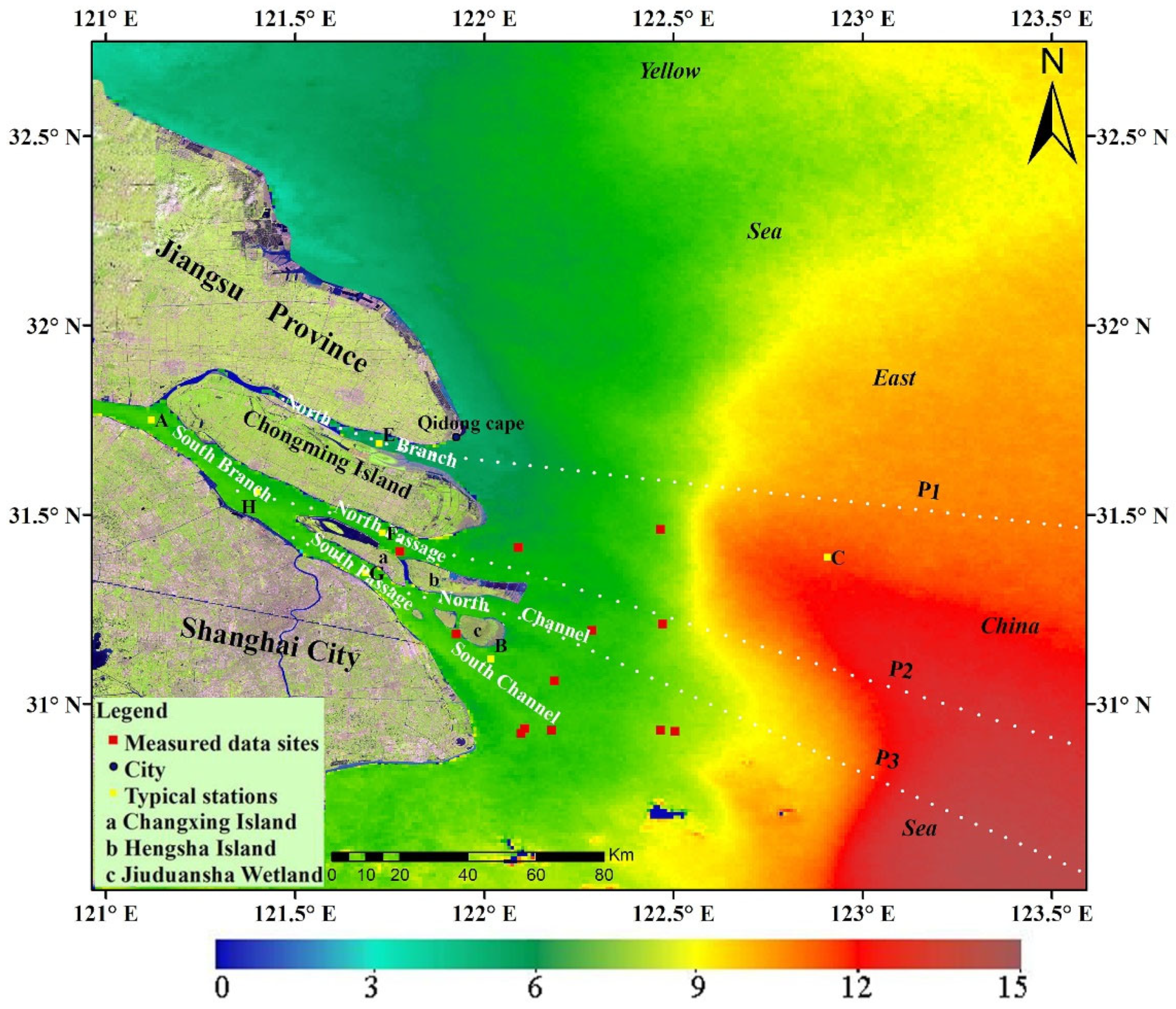
2.1. Study Area
2.2. Cold Weather and Satellite Data
2.3. In Situ SST Measurements
2.4. Construction of the SST Inversion Algorithm
2.5. Determination of Several Important Parameters
2.5.1. Brightness Temperature
2.5.2. Sea Surface Emissivity
2.5.3. Atmospheric Transmittance
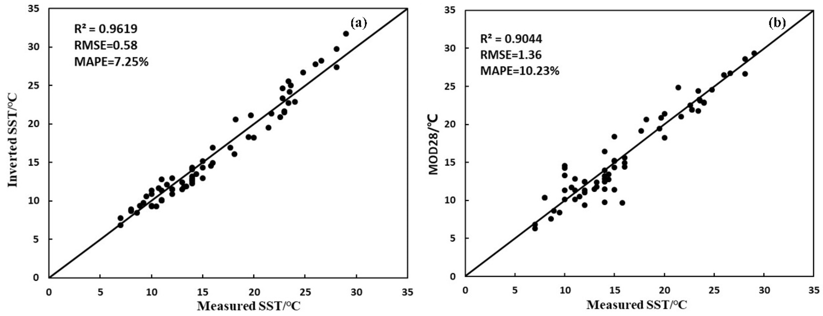
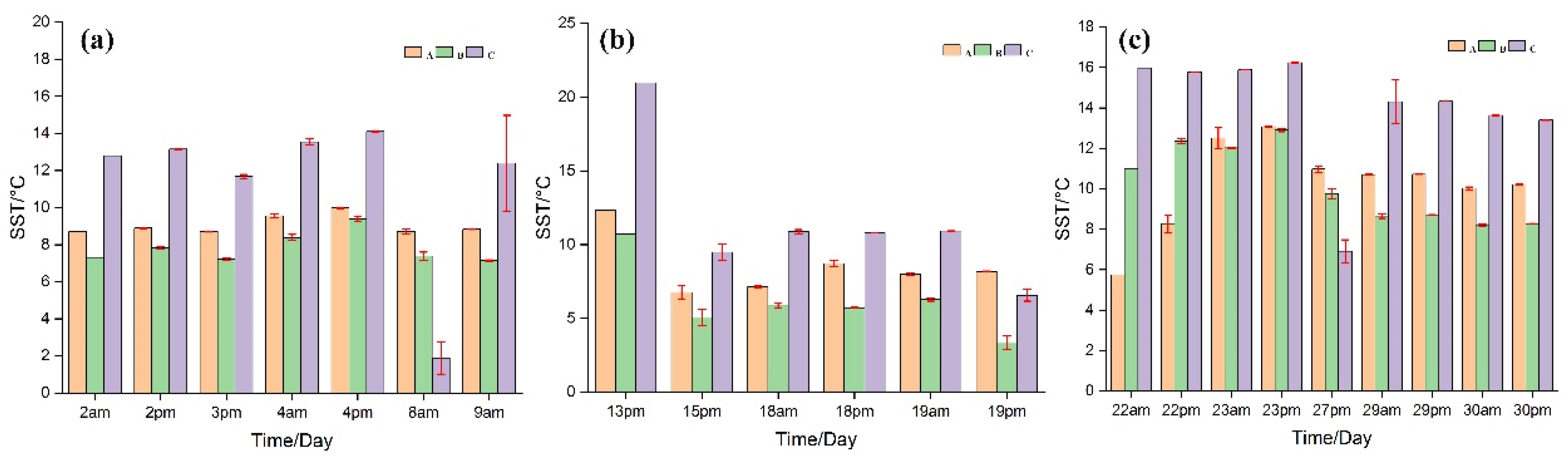
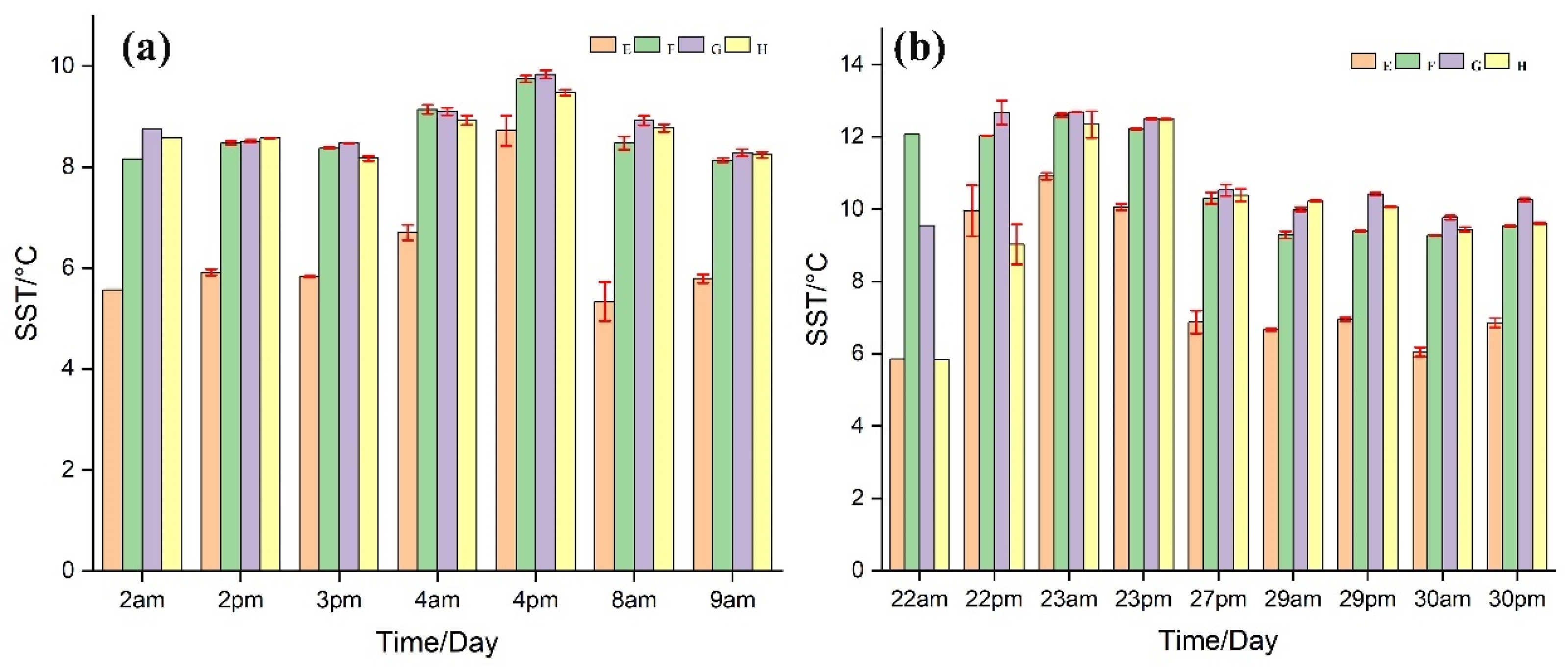
2.6. Accuracy Assessment
2.7. Edge Detection Algorithm Based on Mathematical Morphology
3. Results and Discussion
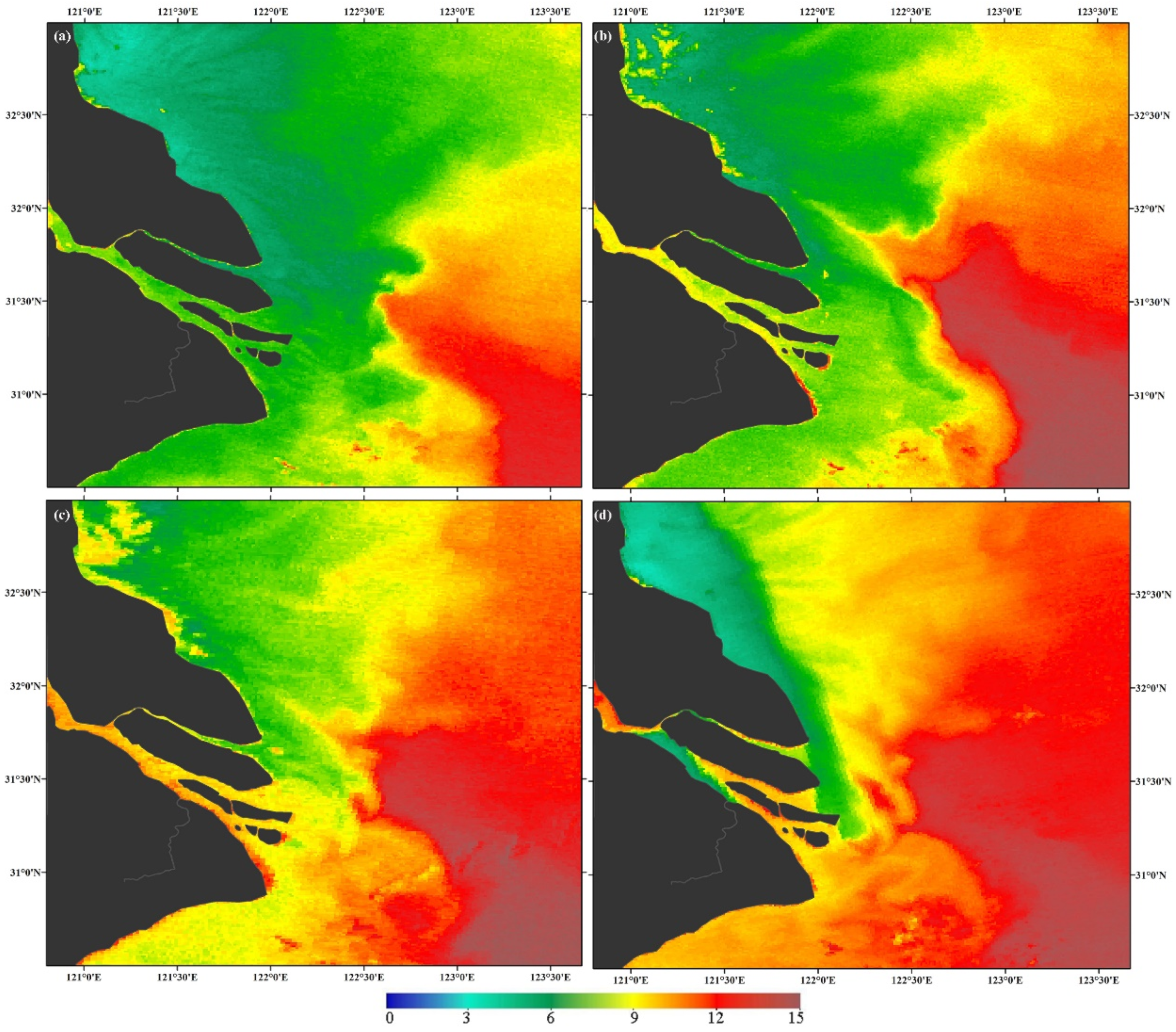
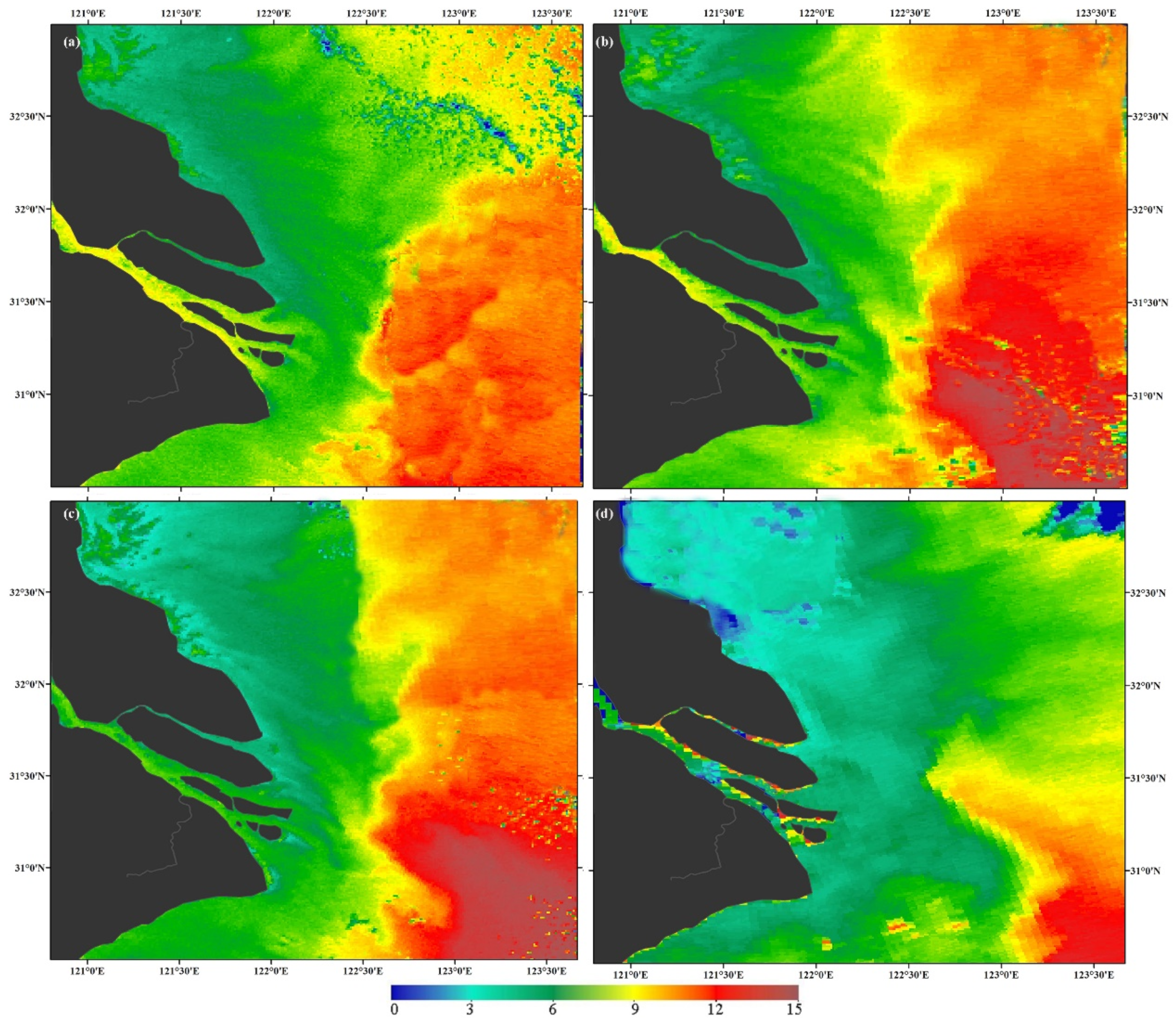
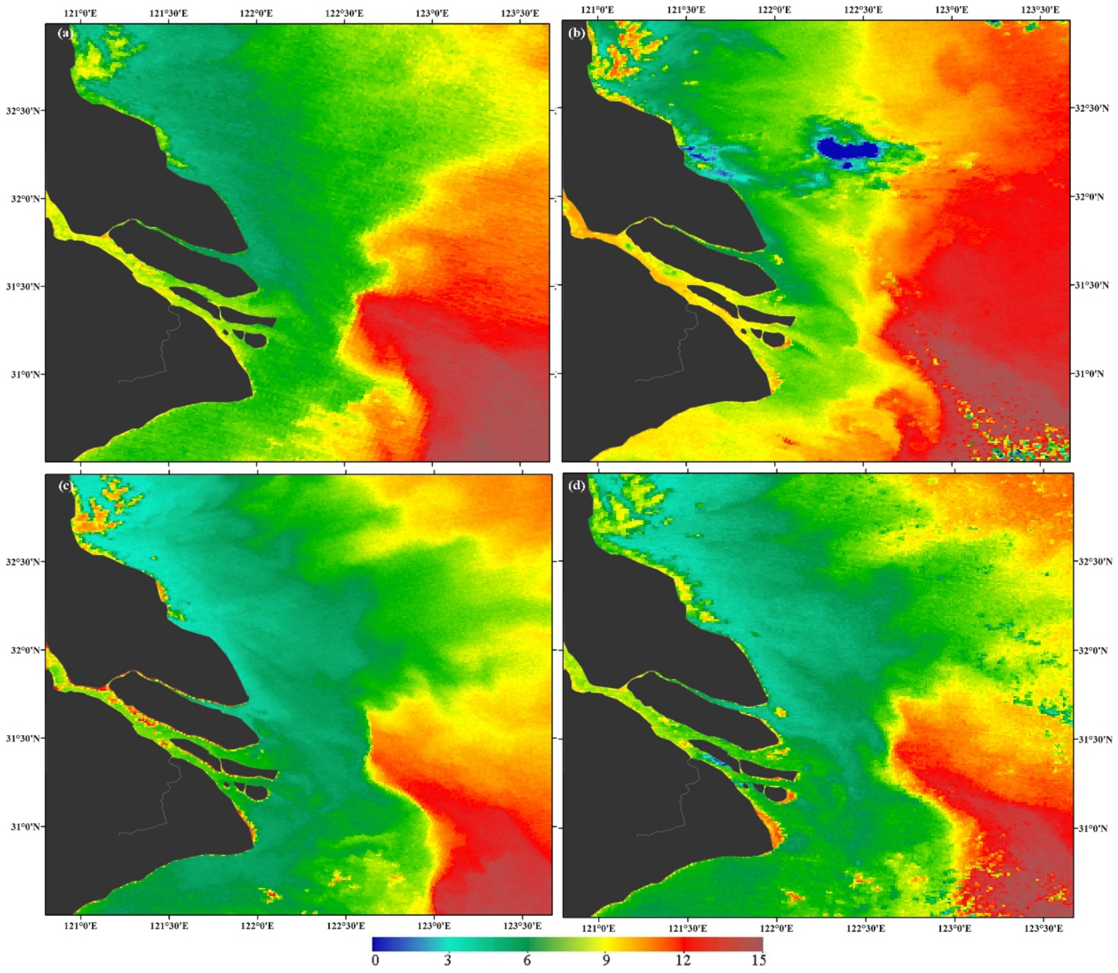
3.1. Characteristics of the Yangtze Estuary’s Temperature Field without Effects from Cold Waves
3.2. Characteristics of the Yangtze Estuary’s Temperature Field before the Arrival of a Cold Wave
3.3. Characteristics of the Yangtze Estuary’s Temperature Field during a Cold Wave
3.4. Characteristics of the Yangtze Estuary’s Temperature Field after a Cold Wave
4. Conclusions
- (1)
- The cold wave alters the temperature field characteristics and the intensity, morphology, and spatial distribution pattern of temperature fronts in the Yangtze Estuary for a short time. Cold water masses along the coast of the north spread out in a tongue-shaped pattern toward the southeast, and a nearshore current interacts with the masses and forms an east–west arc-shaped temperature front in the sea to the east of Chongming Island Beach. The cold wave also interacts with the tongue-shaped warm water masses outside the mouth, which can reach 31°30′~32° N, forming a strong temperature front near 122°E. While the arc-shaped temperature front extends into the outer sea during the cold wave, the boundary becomes more distinct; shear temperature fronts can also be seen in the northern harbor, northern trough, and southern trough waters. Additionally, the strong temperature front moves east to 122°30′~123° E, and the warm water mass begins to retreat south of 31°30′ N. The strong temperature front exhibits irregular edge patterns and scattered patterns as a result of the combined effect of the cold water masses caused by the cold wave and tide, as well as the warm water currents outside the mouth. As cold waves retreat, the cold water mass generated by the cold wave recedes rapidly, continuously, or even vanishes, but the Yangtze estuarine waters maintain their low-temperature characteristics. The boundary of the arc-shaped temperature front becomes increasingly difficult to distinguish. Shear temperature fronts are not observed in the waters of the northern harbor, northern trough, and southern trough. The strong temperature front gradually moves northwest.
- (2)
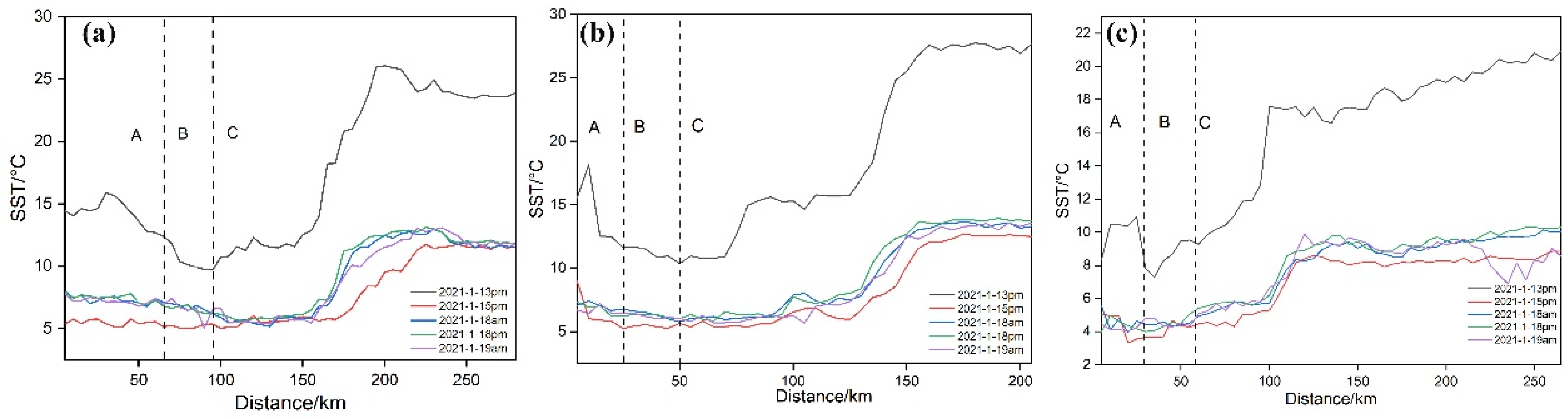
- The cold wave results in significant short-term deviations in the SST of the Yangtze Estuary. The temperature line decreases rapidly with time when a cold wave is present. The cooling outside the mouth reaches a maximum of 12.2 °C, but the cooling inside the mouth is less than 5.5 °C. Inside the mouth, the Northern Branch responds most significantly to the cold wave, with a cooling amplitude of 3.2 °C. After the cold wave, the outside of the mouth warms rapidly, with an average warming up to 5~9 °C, while the inside warms very slowly, averaging only 0.18~1 °C.
- (3)
- Cold waves alter the spatial distribution of low-to-high temperatures in the Yangtze Estuary’s temperature field. Before the cold wave, there is an average temperature gradient of 0.1 °C/km from the inside mouth to the mouth gate and an average temperature gradient of 0.29 °C/km from the mouth gate to the outside mouth. The Yangtze Estuary’s SST is at its lowest level during the cold wave. This results in a temperature gradient of only 0.03 °C/km from inside the mouth to the mouth opening and 0.17 °C/km from the mouth opening to outside the mouth, indicating a pattern of low–lower–higher temperatures. A temperature gradient of 0.19 °C/km is observed from the mouth opening to outside the mouth after the cold wave, while a gradient of 0.05 °C/km occurs inside the mouth and at the mouth opening, which indicates that the spatial pattern of low–high temperature was restored.
- (4)
- Cold waves can significantly influence the strength, morphology, and distribution of the temperature front. In preparation for a cold wave, the temperature gradient of the front is 0.9~1.8 °C/km, with the frontal interface located near 122° 30′ E, and a tongue bulges to the west at 31°30′~32° N. During the cold wave, the temperature gradient is 0.5~1.2 °C/km, the frontal interface gradually moves to 123° E, and the tongue bulging to the west gradually moves to 31°30′ N south. Notably, after the cold wave, the temperature gradient is approximately 0.6 °C/km; the frontal interface of 31°20′~32° N does not vary significantly, but the frontal interface south of 31°20′ N gradually moves to the west, and the tongue bulges to the west and continues to move to 31°~31°30′ N.
Author Contributions
Funding
Institutional Review Board Statement
Informed Consent Statement
Data Availability Statement
Conflicts of Interest
References
- Guan, L.; Chen, R.; He, M. Validation of sea surface temperature from ERS-1 /ATSR in the Tropical and Northwest Pacific. J. Remote Sens. 2002, 6, 63–69. [Google Scholar]
- Cai, R.; Chen, J.; Huang, R. The response of marine environment in the offshore area of China and its adjacent ocean to recent global climate change. Chin. J. Atmos. Sci. 2006, 30, 15. [Google Scholar]
- Wang, D.; Feng, X.; Zhou, L.; Hao, J.; Xu, X. Relationship between blue algal bloom and water temperature in LakeTaihu based on MODIS. J. Lake Sci. 2008, 20, 173–178. [Google Scholar]
- Wang, J.; Wang, J.; Xu, J.; Luan, K.; Yang, Y.; Lv, Y. Characteristics of the Sea Surface Temperature Variation in Adjacent Area of the Yangtze River Estuary. Adv. Mar. Sci. 2020, 38, 624–634. [Google Scholar]
- Sun, Q.; Xue, C.J.; Liu, J.Y.; Xue, C.J.; Liu, J.Y. Spatiotemporal association patterns between marine net primary production and environmental parameters in a view of data mining. Mar. Environ. Sci. 2020, 39, 340–347+352. [Google Scholar] [CrossRef]
- Zhang, C.; Zhou, S.; Zhu, L. Three Algorithms of Sea Surface Temperature Inversion of Daya Bay Based on Environmental Satellite HJ-1B Data. J. East China Inst. Technol. 2013, 36, 88–92. [Google Scholar]
- Hu, H. Impact of the Reservoirs on Downstream Water Temperature Variation Research Based on River Temperature Remote Sensing. Master’s Thesis, Huazhong University of Science & Technology, Wuhan, China, 2018. [Google Scholar]
- Mai, J.; Jiang, X. Analysis of sea surface temperature variations in the Yangtze Estuarine waters since 2000 using MODIS. J. Remote Sens. 2015, 19, 818–826. [Google Scholar]
- Hu, H.; Hu, F. Water types and frontal surface in the Changjiang Estuary. J. Fish. Sci. China 1995, 2, 10. [Google Scholar]
- Chen, J.; Jiang, D.; Zhang, X. Reconstruction of temporal and spatial distribution characteristics of sea surface temperature in the Yangtze River Estuary based on dynamic mode decomposition method. J. Zhejiang Univ. Sci. Ed. 2022, 49, 76–84. [Google Scholar]
- Chen, M.; Shi, S.; Shen, H. Relationship between surface seawater temperature in the Yangtze estuary and El Niño event. Mar. Forecast. 2005, 1, 80–85. [Google Scholar]
- Jiménez-Muñoz, J.C.; Sobrino, J.A. A generalized single-channel method for retrieving land surface temperature from remote sensing data. J. Geophys. Res. Atmos. 2003, 108, D22. [Google Scholar] [CrossRef]
- Sobrino, J.A.; Jimenez-Munoz, J.C.; Paolini, L. Land surface temperature retrieval from LANDSAT TM 5. Remote Sens. Environ. Interdiscip. J. 2004, 90, 434–440. [Google Scholar] [CrossRef]
- Huang, M.; Mao, Z.; Xing, X.; Sun, Z.; Zhao, Z.; Huang, W. A Model for Water Surface Temperature Retrieval from HJ-1B/IRS Data and Its Application. Remote Sens. Land Resour. 2011, 6, 81–86. [Google Scholar]
- Zhou, X.; Yang, X.; Lv, X.; Li, Z.; Tao, Z. The retrieval of the single-channel sea surface temperature using infrared radiative transfer model. J. Trop. Meteorol. 2012, 28, 6. [Google Scholar]
- Tan, Z.; Minghua, Z.; Karnieli, A.; Berliner, P. Mono-window Algorithm for Retrieving Land Surface Temperature from Landsat TM6 data. Acta Geogr. Sin. 2001, 56, 456–466. [Google Scholar]
- McMillin, L.M. Estimation of sea surface temperatures from two infrared window measurements with different absorption. J. Geophys. Res. 1975, 80, 5113–5117. [Google Scholar] [CrossRef]
- Liu, L.; Zhou, J. Using MODIS Imagery to Map Sea Surface Temperature. Geospat. Inf. 2006, 2, 7–9. [Google Scholar]
- Zhang, C.; Zhang, X.; Zeng, Y.; Pan, W.; Lin, J. Retrieval and validation of sea surface temperature in the Taiwan Strait using MODIS data. Acta Oceanol. Sin. 2008, 30, 153–160. [Google Scholar]
- Zhu, L.; Gu, X.; Wang, Q.; Yu, T.; Li, L. A Regional Algorithm to Estimate Sea Surface Temperature in the East China Sea. Remote Sens. Technol. Appl. 2008, 5, 495–499. [Google Scholar]
- Hu, T.; Shen, S.; Shi, C.; Wu, Y.; Wu, Z. Retrieval and Evaluation of 20-year Sea Surface Temperature Sequence Data Sets. Meteorol. Sci. Technol. 2012, 40, 571–577. [Google Scholar] [CrossRef]
- Wan, Z.; Dozier, J. A generalized split-window algorithm for retrieving land-surface temperature from space. IEEE Trans. Geosci. Remote Sens. 1996, 34, 892–905. [Google Scholar]
- Mao, K.; Qin, Z.; Shi, J.; Gong, P. A practical split-window algorithm for retrieving land-surface temperature from MODIS data. Int. J. Remote Sens. 2005, 26, 3181–3204. [Google Scholar] [CrossRef]
- Qin, Z.; Karnieli, A.; Berliner, P. A mono-window algorithm for retrieving land surface temperature from Landsat TM data and its application to the Israel-Egypt border region. Int. J. Remote Sens. 2010, 22, 3719–3746. [Google Scholar] [CrossRef]
- Gao, M.; Tan, Z.; Gao, M.; Zhang, C.; Sebu, L. Calibration of View Angle for Retrieving Land Surface Temperature from the Moderate Resolution Imaging Spectroradiometer (MODIS). Remote Sens. Technol. Appl. 2007, 36, 433–437. [Google Scholar]
- Ri, C.; Liu, Q.; Li, H.; Fang, L.; Sun, D. Improved split window algorithm to retrieve LST from Terra/MODIS data. J. Remote Sens. 2013, 17, 830–840. [Google Scholar]
- Xie, Y.; Ke, L.; Wang, D. Screening of microorganism agents for liriodendron chinense tissue culture seeding and preliminary study on its mechanism. Chin. J. Biol. Control 2018, 20, 281–288. [Google Scholar]
- Hou, J.; He, J.; Jin, X.; Hu, T.; Zhang, Y. Study on optimisation of extraction process of tanshinone II A and its mechanism of induction of gastric cance SGC7901 cell apoptosis. Afr. J. Tradit. Complement. Altern. Med. Ajtcam 2018, 10, 456–458. [Google Scholar] [CrossRef]
- Oates, C.J.; Girolami, M.; Chopin, N. Control functionals for more carlo integration. J. R. Stat. Soc. 2018, 79, 695–718. [Google Scholar] [CrossRef]
- Fortino, G.; Russo, W.; Savaglio, C.; Shen, W. Agent-oriented cooperative smart objects: From IoT system design to implementation. IEEE Trans. Syst. Man Cybern. Syst. 2018, 48, 1939–1956. [Google Scholar] [CrossRef]
- Yin, L.; Kang, Y.J.; Lee, K. Study on the development of smart jewelry in the IoT environment. IEEE Trans. Syst. Man Cybern. Syst. 2018, 9, 19. [Google Scholar] [CrossRef]
- Meneghesso, C.; Seabra, R.; Broitman, B.R. Remotely-sensed L4 SST underestimates the thermal fingerprint of coastal up-welling. Remote Sens. Environ. 2019, 237, 111588–111598. [Google Scholar] [CrossRef]
- Merchant, C.J.; Embury, O.; Bulgin, C.E. Satellite-based time-series of sea-surface temperature since 1981 for climate applications. Sci. Data 2019, 6, 223–241. [Google Scholar] [CrossRef] [PubMed]
- Bai, M.; Wu, H. Characteristics of sea surface temperature in the Changjiang Estuary and adjacent waters based on a Self-Organizing Map. J. East China Norm. Univ. (Nat. Sci.) 2018, 2018, 184–194. [Google Scholar]
- Huang, B.; Deng, R. Pervasive single-channel algorithm-based Yangtze River mouth temperature inversion using HJ-1B data. Anhui Agric. Sci. Bull. 2019, 25, 145–146. [Google Scholar] [CrossRef]
- Ghasemi, A.R. Influence of northwest Indian Ocean sea surface temperature and El Nio–Southern Oscillation on the winter precipitation in Iran. J. Water Clim. Chang. 2020, 11, 1481–1494. [Google Scholar] [CrossRef]
- Ma, W.; Peng, H.; Wu, L.; Meng, H. Interannual variation patterns of sea surface temperature nomaly in the Southern Ocean. Period. Ocean Univ. China 2022, 52, 26–33. [Google Scholar] [CrossRef]
- Brady, F.; Bulusu, S.; Alison, M. Confirmation of ENSO-Southern Ocean Teleconnections Using Satellite-Derived SST. Remote Sens. 2018, 10, 331. [Google Scholar]
- Xu, X.; Dai, J.; Yin, H. The Characteristics of Cold Wave in Shanghai during Recent 20 Years. Atmos. Sci. Res. Appl. 2009, 1, 73–80. [Google Scholar]
- Esaias, W.E.; Abbott, M.R.; Barton, I.; Brown, O.B.; Minnett, P.J. An overview of MODIS capabilities for ocean science observations. IEEE Trans. Geosci. Remote Sens. 1998, 36, 1250–1265. [Google Scholar] [CrossRef]
- Donlon, C.J.; Minnet, P.J.; Gentenmann, C.; Nightingale, T.J.; Barton, I.J. Toward Improved Validation of Satellite Sea Surface Skin Temperature Measurements for Climate Research. J. Clim. 2002, 14, 353–369. [Google Scholar] [CrossRef]
- Qin, Z.; Dall’Olmo, G.; Karnieli, A. Derivation of split window algorithm and its sensitivity analysis for retrieving land surface temperature from NOAA-advanced very high resolution radiometer data. J. Geophys. Res. Atmos. 2001, 10, 22655–22670. [Google Scholar] [CrossRef]
- Zhao, Y. Principles and Methods of Remote Sensing Application Analysis; Science Press: Beijing, China, 2003. [Google Scholar]
- Ottle, C.; Stoll, M. Effect of atmospheric absorption and surface emissivity on the determination of land surface temperature from infrared satellite data. Int. J. Remote Sens. 1993, 14, 2025–2037. [Google Scholar] [CrossRef]
- Liang, S.; Li, X.; Wang, J. Quantitative Remote Sensing: Concepts and Algorithms; Science Press: Beijing, China, 2013. [Google Scholar]
- Niclòs, R.; Valor, E.; Caselles, V.; Coll, C.; Sánchez, J. In situ angular measurements of thermal infrared sea surface emissivity—Validation of models. Remote Sens. Environ. 2005, 94, 83–93. [Google Scholar] [CrossRef]
- Hulley, G.C.; Hook, S.J.; Schneider, P. Optimized split-window coefficients for deriving surface temperatures from inland water bodies. Remote Sens. Environ. 2011, 115, 3758–3769. [Google Scholar] [CrossRef]
- Kaufman, Y.J.; Gao, B.C. Remote sensing of water vapor in the near IR from EOS/MODIS. IEEE Trans Geosci. Remote Sens. 1992, 30, 871–884. [Google Scholar] [CrossRef]
- Mai, J. Remote Sensed Analysis on Sea Surface Temperature Variations in the Yangtze Estuarine Waters since Year 2000. Master’s Thesis, East China Normal University, Shanghai, China, 2015. [Google Scholar]
- Gao, M.F.; Qin, Z.H.; Xu, B. Estimation of the basic parameters for deriving surface temperature from MODIS data. Arid Zone Res. 2007, 24, 7. [Google Scholar]
- Minnett, P.J.; Brown, O.B.; Evans, R.H.; Key, E.L.; Kearns, E.J.; Kilpatrick, K.; Kumar, A.; Maillet, K.A.; Szczodrak, G. Sea-surface temperature measurements from the Moderate-Resolution Imaging Spectroradiometer (MODIS) on Aqua and Terra. In Proceedings of the IEEE International Geoscience & Remote Sensing Symposium, Anchorage, AK, USA, 20–24 September 2004. [Google Scholar]
- Shimada, T.; Sakaida, F.; Kawamura, H.; Okumura, T. Application of an edge detection method to satellite images for distinguishing sea surface temperature fronts near the Japanese coast. Remote Sens. Environ. 2005, 98, 21–34. [Google Scholar] [CrossRef]
- Lian, J.; Wang, K. An Image Edge Detection Method Based on Multi-scale Morphology. Comput. Eng. Appl. 2006, 42, 3. [Google Scholar]


| Water Vapor Content w (g/m2) | Atmospheric Transmittanceτ | R2 |
|---|---|---|
| Winter 0.0~1.4 | τ31 = 0.9295 − 0.0939w τ32 = 0.9413 − 0.1009w | 0.9943 0.9904 |
| MODIS Band | Temperature Correction Function | Temperature Interval |
|---|---|---|
| B31 | T31 > 318 K 278 < T31 < 318 T31 < 278 K | |
| B32 | T32 > 318 K 278 < T32 < 318 T32 < 278 K |
Disclaimer/Publisher’s Note: The statements, opinions and data contained in all publications are solely those of the individual author(s) and contributor(s) and not of MDPI and/or the editor(s). MDPI and/or the editor(s) disclaim responsibility for any injury to people or property resulting from any ideas, methods, instructions or products referred to in the content. |
© 2023 by the authors. Licensee MDPI, Basel, Switzerland. This article is an open access article distributed under the terms and conditions of the Creative Commons Attribution (CC BY) license (https://creativecommons.org/licenses/by/4.0/).
Share and Cite
Chen, R.; Jiang, X.; Chen, J. Satellite Imagery Recording the Process and Pattern of Winter Temperature Field in Yangtze Estuary Interrupted by a Cold Wave. Atmosphere 2023, 14, 479. https://doi.org/10.3390/atmos14030479
Chen R, Jiang X, Chen J. Satellite Imagery Recording the Process and Pattern of Winter Temperature Field in Yangtze Estuary Interrupted by a Cold Wave. Atmosphere. 2023; 14(3):479. https://doi.org/10.3390/atmos14030479
Chicago/Turabian StyleChen, Ruirui, Xuezhong Jiang, and Jing Chen. 2023. "Satellite Imagery Recording the Process and Pattern of Winter Temperature Field in Yangtze Estuary Interrupted by a Cold Wave" Atmosphere 14, no. 3: 479. https://doi.org/10.3390/atmos14030479
APA StyleChen, R., Jiang, X., & Chen, J. (2023). Satellite Imagery Recording the Process and Pattern of Winter Temperature Field in Yangtze Estuary Interrupted by a Cold Wave. Atmosphere, 14(3), 479. https://doi.org/10.3390/atmos14030479