Abstract
Temperature inversions prevent the mixing of air near the surface with the air higher in the atmosphere, contributing to high concentrations of air pollutants. Inversions can be identified by sampling temperature data at different heights, usually done with radiosondes. In our study, we propose using the SMIXS clustering algorithm to cluster radiosonde temperature data as longitudinal data into clusters with distinct temperature profile shapes. We clustered 8 years of early morning radiosonde data from Ljubljana, Slovenia, into 15 clusters and investigated their relationship to PM pollution. The results show that high PM concentrations (above 50 /, which is the daily limit value) are associated with early morning temperature inversions. The highest concentrations are typical for winter days with the strongest temperature inversions (temperature difference of 5 or more in the inversion layer) while the lowest concentrations (about 10 /) are typical for days with no early morning temperature inversion. Days with very strong temperature inversions are quite rare. We show that clustering temperature profiles into a distinct number of clusters adds to the interpretability of radiosonde data. It simplifies the characterization of temperature inversions, their frequency, occurrence, and their impact on PM concentrations.
1. Introduction
The temperature usually decreases with increasing altitude. In this article, we discuss temperature inversions, which occur when there is a layer of air with increasing temperature and a layer of cold air trapped underneath [1]. The pocket of cold air near the ground does not mix with the warmer air above it, trapping air pollutants near the ground as well. The air near the ground becomes very stable, with high humidity and low wind.
A temperature inversion can start at the ground (surface inversion) or higher (an elevated inversion) [2]. On cold days, especially at night when surface cooling is fast and the air above it becomes warmer (it does not emit heat back as fast as the surface), temperature inversions form. These are called surface inversions and are common in valleys and basins where steep slopes contribute to the accumulation of cold air near the ground [3]. An elevated inversion occurs when the pocket of cold air is not near the ground but higher in the atmosphere. It is usually caused by the advection of warm air from low altitudes or warm air moving above a region [4]. Temperature inversions can be assessed by conducting vertical sounding, which involves measuring air temperature, humidity, wind speed, and direction at a specific location and different altitudes. This is most commonly done using a radiosonde attached to a weather balloon.
One of the main air pollutants largely influenced by temperature inversions is particulate matter (PM); it can harm human health when inhaled [5], especially affecting the cardiovascular and respiratory systems. PM consists of particles with a diameter of less than 10 μm, forming a heterogeneous mixture of tiny solid and liquid particles suspended in the air [5]. Its composition varies in size and chemical composition [6]. These particles can remain suspended for a long time [6] and can travel long distances [7,8]. Temperature inversion affects air pollutant concentrations significantly, which has been studied in a large number of works [1,3,9,10,11,12,13,14,15,16,17].
Many studies dealing with low-level inversions only identify the first inversion layer [18,19,20]. Huang et al. [18] and Guo et al. [21] identified low-level temperature inversions over China between 2011 and 2018 and between 2011 and 2017, respectively, using radiosonde data. In 2022, Li et al. [20], and in 2015, Li et al. [12] analyzed radiosonde data taken between 2001 and 2010 and between 2010 and 2015 from the Southern Great Plains. To process radiosonde data, these works used a procedure based on the first derivative [22]. The profile of the first derivative was scanned upwards from the surface to identify the points where the sign of the first derivative changed. As radiosonde data can be jumpy, a threshold was set to join two apparent layers (when the change in sign of the first derivative was short). This method allowed for the identification of the height and thickness of temperature inversions.
Clustering was used before for pre-processing radiosonde data for bias correction [23]. According to [24], it proved to be efficient in clustering diurnal cycles of temperature changes. In our work, instead of clustering trajectories depicting the change in temperature with time (as in [24]), we clustered trajectories of temperature changes with altitude. Truong et al. [25] used k-means clustering to cluster temperature profiles measured above the Southern Ocean according to a few extracted values to study the marine atmospheric boundary layer. Clustering enabled them to define the seasonality of different profiles. Clustering has also been used extensively for the analysis of meteorological parameters and air pollution [26,27]. Nidzgorska-Lencewicz and Czarnecka [28] used the methodology described in [29], which is very similar to [22], to assess the height, strength, and base height of the inversion. They clustered the attributes according to the corresponding PM concentrations. Clustering techniques have also been used for clustering air mass trajectories [8,30,31], where they proved to be great tools for processing many trajectories.
The aim of our work is to propose a method to increase the interpretability of radiosonde data and to make the analyses feasible even when dealing with large amounts of data. We wanted to preserve much of the information from radio-sounding (rather than condense it to a few points). The interpretability of clustered air mass trajectories was key to this approach. As seen in related work, atmospheric-sounding data can be quite tedious to process, as they are two-dimensional. Typically, the temperature data are plotted, and the temperature inversions are assessed manually, which is quite inconvenient when processing a large amount of data. The automated method of choice for processing radiosonde data is usually [22], which typically condenses trajectory data to a few numbers.
By using the Ljubljana, Slovenia, case study, we wanted to show that radiosonde data can be efficiently clustered using a novel non-parametric regression-based clustering algorithm named smooth mixture splines (SMIXS) [32]. We hypothesized that by clustering vertical temperature profiles as longitudinal data we could identify distinct clusters of temperature profiles that are characteristic of days with high PM concentrations. Temperature inversions have been known to affect pollutant concentrations in Ljubljana [33] but their characteristics have never been thoroughly evaluated. In general, inhabited valleys and bases are prone to air pollution in the winter because of high emissions and unfavorable meteorological conditions (temperature inversion, low wind conditions) and Ljubljana is a typical example of a city lying in a basin surrounded by mountains and exhibiting continental climate. We also hypothesized that the shapes of the temperature profiles differ significantly between different seasons, but do not differ significantly between different years. We thought that—especially in the winter—strong temperature inversions (with large differences between the minimal and maximal temperatures in the inversion layer) are present. Each study of the factors affecting PM concentrations is very important because PM pollution is the main air quality issue in Slovenia [8,33,34].
The remainder of the paper is structured as follows. We first present the investigated data in Section 2.1 and data preprocessing in Section 2.2. We present the SMIXS algorithm in Section 2.3 and show how we use it for clustering our data in Section 2.4. In Section 3, we describe the clustering of radiosonde data from Ljubljana and investigate their relationship to PM concentrations. We summarize our study and the main findings in Section 4.
2. Data and Methodology
2.1. Data
Ljubljana is the capital of Slovenia. It has approximately 300 thousand inhabitants and it lies in a basin surrounded by mountains at an altitude of 295 m. Temperature inversions and low temperatures are very common in the winter, which affects air quality [15,33,34]. On days when the height of the temperature inversion is low (below 400 m), PM concentrations can exceed the daily limit value of 50 μg/ [11,33]. There are also episodes of persistent temperature inversions similar to the Grenoble case study [35]. Similar conditions are typical for all Slovenian towns lying in valleys and bases in the continental climate and are common in most of central Europe. The Slovenian Environment Agency (ARSO) [36] is responsible for weather prediction, meteorological measurements, and air quality measurements. It also performs air quality prediction.
ARSO performs atmospheric-sounding [37] every day, early in the morning (at around 5) using high-resolution GPS radiosondes. They measure temperature (temperature profile), air humidity, and wind speed at different altitudes until a maximum altitude of around 19,913.7 m above sea level (m.a.s.l.). The radiosonde samples temperatures every second. As temperature inversions have a greater impact on air quality when they occur closer to the ground, we used 100 temperature measurements from altitudes ranging from approximately 300 m.a.s.l. (the altitude of Ljubljana) to 750 m.a.s.l. By focusing on lower altitudes, we ensured that we captured the most relevant air layer [11,38] that affected air pollution. The height of low-level temperature inversions is usually between 75 and 150 m above the ground [1,17,39]. Prasad et al. [38] showed that the vertical distribution of aerosols is constrained by temperature inversions and that the boundary layer altitude is not the deciding factor in most cases.
We use the term temperature inversion height to denote the point where the temperature stops increasing with increasing altitude and starts decreasing (the “end” of temperature inversion); temperature inversion base is the height at which the temperature starts to increase with increasing altitude; temperature inversion strength is the maximal difference in temperature in the inversion layer [4].
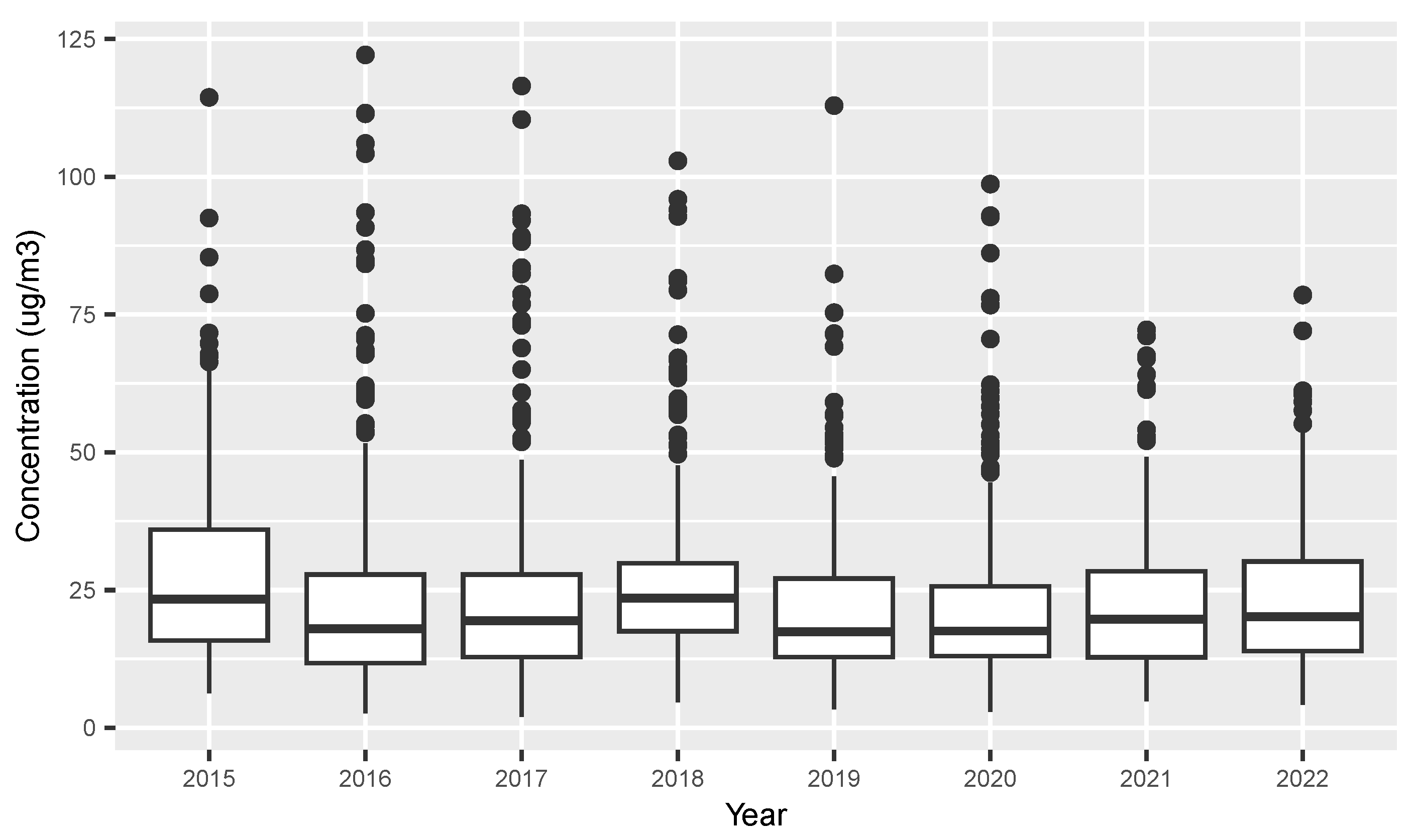
The investigated PM daily concentrations were sampled at the same location as the starting point for atmospheric-sounding. PM concentrations were assessed as daily mean values measured with the reference method [40] that comprise active sampling and subsequent gravimetric analyses in the ARSO chemical–analytical laboratory. We focus on PM measurements from 2015 to 2022. Figure 1 shows the measured PM concentrations for different years and Figure 2 shows the distributions of the concentrations for different months. In this paper, when we discuss high and low PM concentrations, we refer to Figure 2. The investigated PM concentrations were also provided by ARSO. Table 1 shows the number of pairs of temperature profiles and PM concentrations available for each month while Table 2 shows the available pairs for each year. In total, we used 2197 clustered temperature profiles.
Figure 1.
The PM concentrations used in our study for each year. The concentrations for days where sounding data were missing were removed.
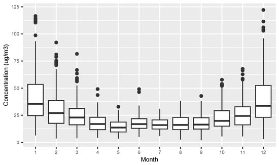
Figure 2.
The PM concentrations used in our study for each month. The concentrations for days where sounding data were missing were removed.

Table 1.
Number of temperature profiles and PM concentration pairs available for each month.

Table 2.
Number of temperature profiles and PM concentration pairs available for each year. Not all of the data for 2022 were available at the time this study was conducted.
2.2. Pre-Processing of Atmospheric-Sounding Data
Atmospheric-sounding data are not always reliable and, therefore, have to be pre-processed before further analysis can take place. Since our altitude interval of interest spanned from 300 to 750 m.a.s.l., samples that did not reach the maximum height were discarded. Following this, we discarded samples where the difference between consecutive measurement altitudes was larger than 50 meters and where the temperature between consecutive measurements changed by more than 8 . We believe these are reasonable constraints. Measurements taken by the radiosonde are typically conducted very frequently (every second) as the device ascends the atmosphere. Therefore, large deviations in temperature or measurement altitudes are highly unlikely and usually denote hardware issues or are consequences of other interferences. Altitudes at which temperature measurements are conducted by radiosondes vary between individual sounding samples. This means we cannot directly compare raw measurements between samples since they are not taken at the same altitudes. Therefore, we linearly interpolated measurements from each atmospheric-sounding sample to a common set of 100 altitudes, equally spaced between 300 and 750 m in altitude. We found that 100 measurements resulted in a good resolution, retaining key changes in temperatures while not being computationally overbearing.
The obtained post-processed data were again checked for abnormal temperature deviations as errors could still occur. For example, interpolations might exhibit unexpected behaviors if many measurements are captured over a small difference in altitude, resulting in “jumpy” interpolated values.
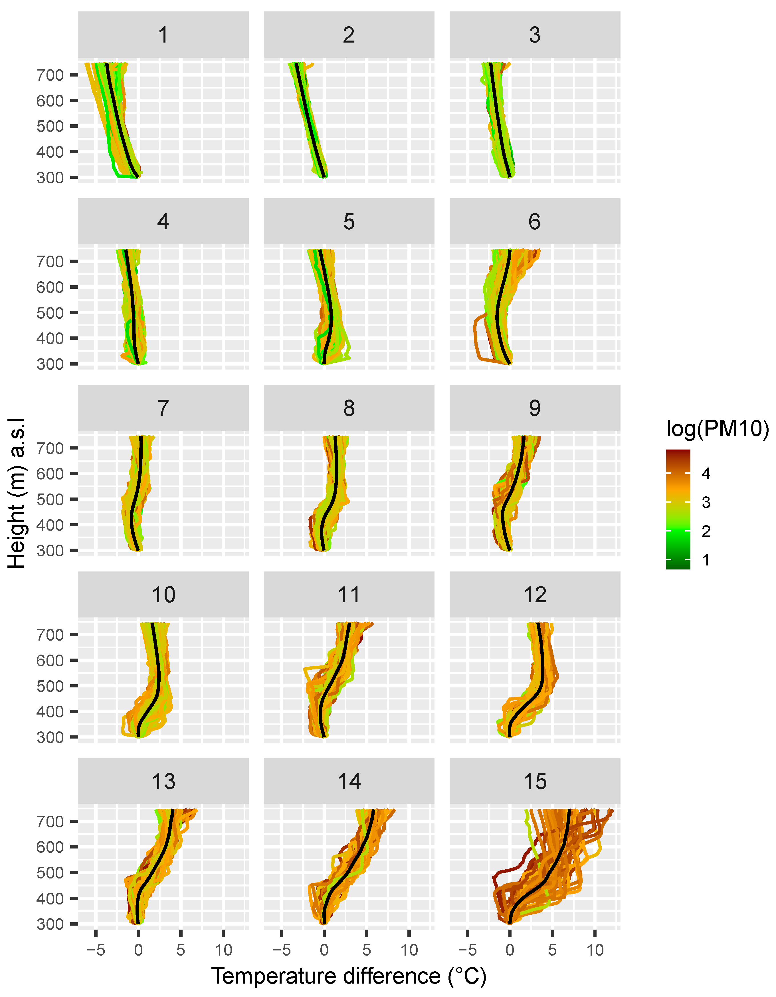
When clustering the temperature profiles, we settled all of the trajectories so they had the same starting point. We only looked at the change in the temperature from the ground up and disregarded the absolute temperature (see Figure 3). In this way, we clustered the shapes of the trajectories disregarding the actual temperatures.

Figure 3.
Temperature profiles from 2015 to 2022 clustered in 15 different clusters. The color of the temperature profile represents the logarithm of the measured PM concentration on the same day the vertical temperature profile was measured. All temperature profiles are settled so they all start at 0. An increase in temperature with height has a positive slope.
2.3. SMIXS
SMIXS [32] is a probabilistic algorithm for simultaneous clustering and regression; it is tailored for processing longitudinal data with multiple latent clusters. SMIXS extends the Gaussian mixture model (GMM) approach, resulting in a probabilistic clustering of the dataset. Therefore, each data sample is clustered based on its probability of belonging to a specific cluster. The SMIXS algorithm is based on the work by [41] and it differentiates itself from the original work by including speed-ups to crucial computational bottlenecks and an improved variance estimator, resulting in more stable and efficient performance. Additionally, SMIXS can produce smooth mean cluster curves describing the temporal development of the longitudinal data it processes. Because real word measurements usually include noise, SMIXS uses smoothing splines to remove the effects noise would have on the ultimate cluster mean estimates. The degree of smoothing is determined using cross-validation and is dynamically adapted depending on the amount of noise in the dataset, on a per-cluster level. The smoothing procedure requires additional operations and, therefore, negatively impacts computational complexity. If the processing speed is important, one can fix the amount of smoothing applied to individual clusters, resulting in computational performance comparable to that of the base GMM, while still retaining the smoothing effects of SMIXS, albeit the smoothing might not be optimal. Therefore, there is a trade-off between optimizing for smoothness and the computational complexity of the algorithm.
To successfully analyze data using SMIXS, multiple initializations are required to produce reliable results. This is because SMIXS iteratively improves the initial clustering until convergence using the expectation-maximization algorithm [42]. Therefore, in large datasets with multiple latent clusters, SMIXS can produce different estimated clusters depending on the initialization. Since we are interested in one estimated clustering only, we select the one that maximizes the log-likelihood. However, we still have to determine the number of latent clusters in the dataset that SMIXS has to estimate. This is a consequence of SMIXS extending GMM, where the user is required to specify the number of clusters in the dataset. How to determine the appropriate number of clusters in a dataset is an open research problem. Based on the suggestion of [41], we used the Bayesian information criterion (BIC) [43] to estimate the number of latent clusters by selecting the model that minimized the criterion. This procedure is heuristic. However, it provides a good estimate on the number of optimal clusters. In essence, it strikes a specific balance in the trade-off between interpretability (too many clusters are hard to interpret) and cluster homogeneity.
SMIXS exhibits improvements in terms of regression accuracy and clustering performance in terms of regression and clustering accuracy compared to GMM when tested on a synthetic dataset. Its outperformance was especially evident when a large amount of noise was present (see [32]. SMIXS also showed good performance when clustering the COVID-19 time series [44], where we studied the similarity of COVID-19 development trends between different European countries. The latter example gave us the idea to use SMIXS for clustering atmospheric-sounding data. Noise is a common issue in all environmental measurements [45]. Due to the smoothing nature of SMIXS, we likewise believed that it would outperform other clustering algorithms, such as k-means, in terms of the regression accuracy of cluster mean estimates. This is because k-means does not explicitly handle the issue of noisy datasets and would therefore be subject to the same constraints as GMM.
2.4. Clustering Atmospheric-Sounding Data
Each trajectory composed of 100 temperature data (vertical measurements) represents one clustering instance. First, we assessed the adequate number of clusters with the BIC (BIC). We observed the plotted BIC curve for an increasing number of clusters from 2 to 19 and chose the number of clusters; after which, the decrease in BIC was not significant enough (where the BIC curve flattens, see Figure A1 in the Appendix A). In our case, we set a threshold of three percent in the BIC decrease when we increased the number of clusters. As this procedure is very time-consuming, we only used data from 2017 to 2019 in this part.
The estimation of the “optimal” number of clusters took 100 min to complete with 50 initializations per cluster number on a system with an Intel i9-9700K processor. In each iteration, we retained the best initialization in terms of the BIC.
After determining the number of clusters as described above, we reran the SMIXS clustering using the selected number of clusters and all of the temperature profiles (2015–2022) that passed the pre-processing phase (see Section 2.2). This took approximately 20 min. SMIXS assigned the most probable cluster to each trajectory and it gave us the typical temperature profile (centroid) for each cluster.
To assess if some temperature profiles were typical for different seasons, e.g., summer temperature profiles differed from winter temperature profiles, we assessed the occurrences of each cluster in each month for the period 2015–2022.
3. Results and Discussion
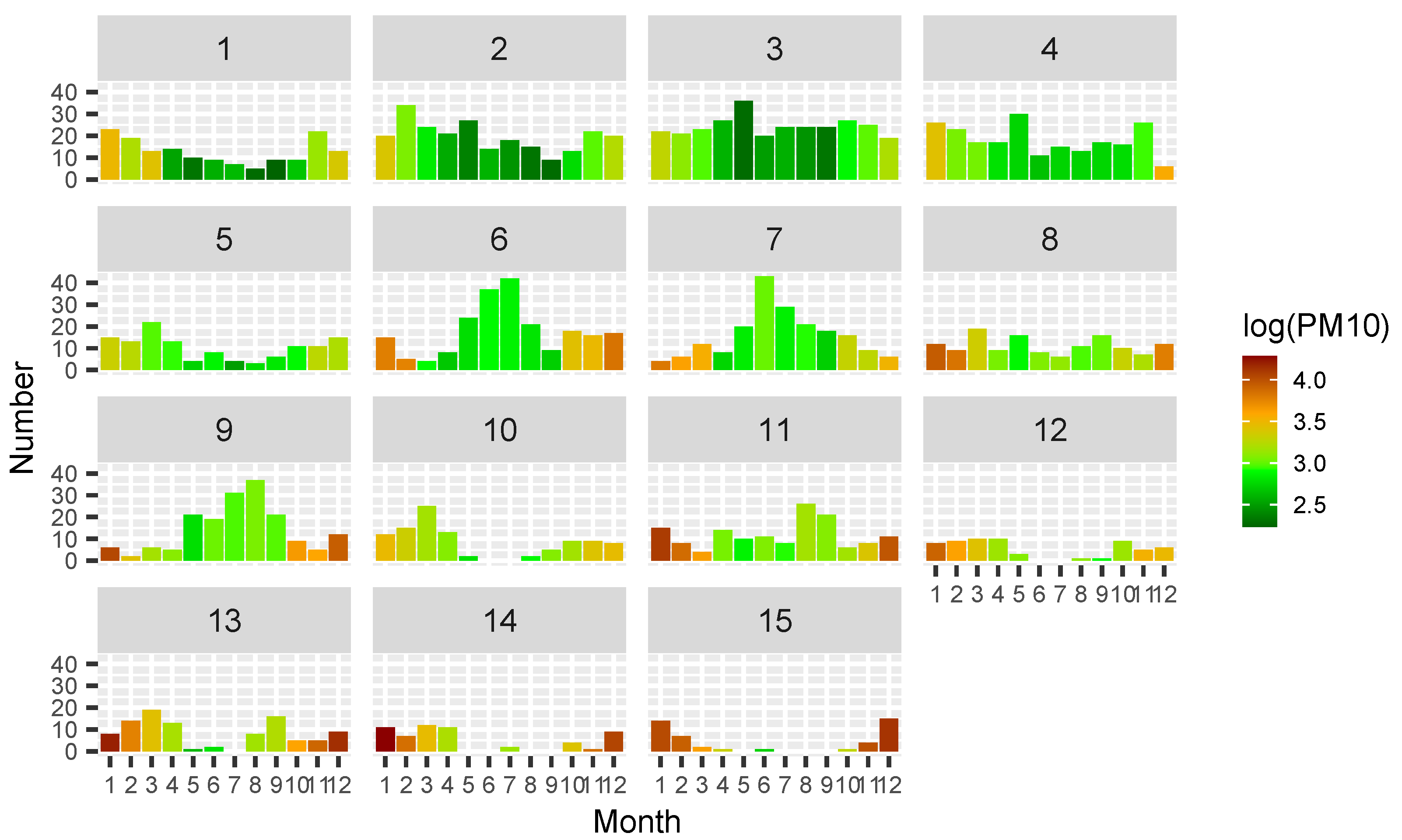
We determined the optimal number of clusters for our data to be 15. Figure 3 displays the 15 clusters along with their corresponding temperature profiles. For each cluster, we calculated the average slope of the cluster centroid, which is the centroid of the Gaussian distribution and the regression result. We then ordered the clusters based on their average slope (refer to Table A2 in the Appendix A) so that the clusters in Figure 3, Figure 4 and Figure 5 are arranged from the cluster with no temperature inversion to the one with the strongest temperature inversion. The average slope refers to the average temperature change between consecutive measurements, i.e., the temperature change every 4.5 m. Figure 3 only displays the temperature changes, with all trajectories starting at zero. A positive slope from zero upwards indicates increasing temperature with elevation. The colors of the trajectories represent the logarithm of the measured PM10 concentrations. As PM10 concentrations typically follow a log-normal distribution, we plot the logarithm of the concentrations. Figure 4 shows the trajectory distribution across different clusters in different months, with colors representing the logarithm of the mean concentrations for each month–cluster combination.
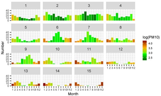
Figure 4.
Histograms of the number of different temperature profiles per month for each cluster. Colors depict the logarithm of the mean concentration observed in a month in a cluster.
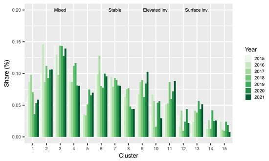
Figure 5.
Percentage of cluster instances (share in %) for each year.
To characterize the clusters, we observed the calculated slopes for each centroid temperature profile and assessed the rate of change of the temperature at different heights. In Figure 3, the clusters that do not exhibit a temperature inversion (clusters 1–4) and the clusters where the centroid has a negative slope through the observed heights correspond to lower PM concentrations on average. Clusters that correspond to a very stable atmosphere are the clusters with temperatures almost constant through the observed air layer (alternating slope between −0.05 and 0.05 with a mean of 0), i.e., clusters 5, 6, and 7. Clusters that exhibit an elevated temperature inversion are clusters where the slopes of their centroids are at first negative and then positive, i.e., clusters 8, 9, and 11. Clusters showing stable situations and the ones representing elevated temperature inversions comprise a mixture of higher and lower PM concentrations. Clusters that correspond to surface inversions are the clusters where the slopes of their centroids are positive throughout the observed air layer (clusters 10, 12, 13, 14, and 15). These clusters exhibit the highest PM concentrations. In clusters 10 and 12–15, we can observe that the stronger a morning temperature inversion is, the higher the corresponding PM concentrations are on average. In Figure 3 and Table 3, we can also observe that in all clusters there are some PM concentrations that do not conform to the rule “the stronger the temperature inversion the higher the concentrations”. This is because temperature inversion is one of the most important (but not the only) factors influencing PM concentrations. The depicted PM concentrations are daily values defined as the mean concentration from 0:00 one day to 0:00 the following day, while the temperature inversion is measured only once, i.e., early in the morning. Strong morning temperature inversions are linked to persistent temperature inversions when the weather is stable [15,35]. Largeron and Staquet [35] found that during persistent temperature inversions, there was a strong surface inversion close to the ground in Alpine valleys. Similar but less severe conditions can be observed in Ljubljana, which lies in a sub-alpine basin. However, during the day, the weather can change, e.g., the wind can intensify or it can rain, which dilutes PM. Therefore, daily concentrations can be low even though there is a strong temperature inversion in the morning. Another cause of the discrepancy is likely the fact that the most important factor impacting PM concentrations is PM emissions. Emissions in Ljubljana are higher in the winter [46] because of indoor heating, which substantially contributes to PM. Usually, the colder it is, the more PM emissions there are. This affects PM concentrations independent of the dispersion situation in the city (temperature inversion). According to the latest Slovenian emission inventory 70% of PM, anthropogenic emissions are attributed to households [34] and the main source of PM households is indoor heating, which is present between October and April.

Table 3.
The number of temperature profiles clustered in each cluster; mean and median PM concentrations for each cluster and the standard deviation of the PM concentrations in each cluster.
The relationship between concentrations and seasons can be observed in Figure 4. Winter months have higher concentrations regardless of the temperature profiles. The lowest PM concentrations are measured during the summer and spring months (see Figure 2 for typical summer and spring concentrations) when the atmosphere is well mixed. Trajectories with decreasing temperature profiles (clusters 1–4) are common throughout the year and are typical for unstable weather conditions (wind, rain). However, such profiles are more frequent in the summer. On the other hand, clusters 6, 7, and 9 depict very stable situations or elevated inversions, which are more common in the summer. These profiles are linked to much higher concentrations in the winter than in the summer, likely due to increased PM emissions in the winter, which agrees with observations from Poland [17]. The strongest inversions are present mostly during the winter months (clusters 14 and 15), and weaker temperature inversions are more frequent in autumn and spring (clusters 10, 12, and 13). Clusters showing temperature inversions are not observed in the summer; the ones in Figure 4 are most likely a result of undetected outliers in the data. The early morning temperature inversions are common also in the warmer months, but they are more commonly elevated inversions, not strong, and break up easily, so they are not associated with high PM concentrations. Similarly, Xu et al. [4], Huang et al. [18] found that surface inversions were typical for winter months, while elevated inversions were more common in the summer months in two cities in the north of China.
Table 3 shows the mean and median PM concentrations per cluster with the associated standard deviations. The standard deviations for all clusters are large. As described before, PM concentrations are affected by many factors, not only by morning temperature inversions, so the same temperature profiles can be attributed to different PM concentrations. From Table 3, there is also a trend evident; the mean and median cluster concentrations (with a few exceptions) increase from clusters 1 to 15. The mean and median values are the lowest for clusters 1–4 (no inversion), are higher for clusters 5–9 and 11 (stable and elevated inversion), and are the highest in clusters 12–15 (surface inversion), with some even in cluster 11.
In Figure 4, it is evident that for the same temperature profile, the concentrations in the summer are lower than in the winter, probably due to increased emissions and lower solar radiation. In Table 3, the median values are also lower than the mean values, which indicates that the values in clusters are not normally distributed. PM concentrations are generally gamma-distributed (limited by 0 with a heavy tail). Clusters display skewed distributions with a heavy tail toward higher concentrations.
From the Ljubljana example, by clustering temperature profiles, we were able to analyze temperature inversions and their relationships to PM concentrations for a period of almost 8 years (from January 2015 to the end of June 2022) quite easily. Without clustering the data, a similar analysis would be much more time-consuming and the result would be more difficult to interpret.
Another application of the clustering of radiosonde data involves clustering the temperature profiles and then observing trends of different shapes of temperature profiles through the years (see Figure 5). Figure 5 shows that clusters are not identically represented between the years, but the yearly distributions between clusters or types of clusters are very similar in the observed period. The most represented are the clusters depicting a mixed atmosphere, especially clusters 2 and 3. In the observed period, there is no evident trend in cluster manifestation. A 7-year period is likely not enough to establish a long-term trend, but clustering temperature profiles could enable us to do a similar analysis for a longer period and help us establish if there is a long-term trend in the occurrences of temperature inversions and their strengths. The cluster depicting the strongest temperature inversions is the least frequent in all of the years supporting the hypothesis that strong temperature inversions are rare. In this part of the analysis, we removed data from 2022 because data were available only until June.
4. Conclusions
In our article, we proposed clustering temperature profiles obtained from radiosondes to study the relationship between temperature inversions and air pollutant concentrations. We chose the clustering SMIXS algorithm due to its flexibility and statistical interpretability. We analyzed the Ljubljana early morning radiosonde data provided by ARSO, clustered it into 15 clusters, and examined the relationship between PM concentrations and the assigned cluster.
As shown in the Ljubljana case study, clustering temperature profiles facilitated the interpretation of the relationship between temperature profiles and PM. It also allowed for the evaluation of more frequent temperature profile shapes in different seasons, which is empirical evidence of predominant temperature profile shapes in different seasons, particularly in winter, in Ljubljana. In most related works, only some parameters of temperature profiles were investigated [12,18,20,21], and in [47], surface-based temperature inversions were assessed as the difference in temperature at 2 and 88 m clustering. Compared to these methods, clustering entire profiles enabled us to preserve more information and enabled a more refined interpretation. Clustering also enables the characterization of temperature profiles based on objective criteria without human decision-making. Cluster centroids generated by SMIXS are also smooth, making them easier to interpret. When clustering with SMIXS, we did not have to deal with individual profiles where the temperature profile is usually not smooth.
The main conclusions from the cluster analysis were in line with the related work about the relationship between temperature inversions and PM concentrations [1,7,10,11,12,14]. Morning surface temperature inversions are associated with high PM concentrations (depicted in red and orange in Figure 3 and Figure 4, which corresponds to approximately above 40 μg/), especially in the winter. The strongest temperature inversions (cluster 15; corresponding to approximately a temperature difference of 8 at 750 m) were present only in the colder months and were rare. The most representative temperature profiles in Ljubljana showed decreasing temperatures with the altitude (mixed atmosphere). These profiles are associated with the lowest PM concentrations (around 10 μg/). Such situations are common year-round (not only in the summer). Morning temperature inversions in the summer are not associated with high PM concentrations probably because of lower summer PM emissions. The conclusions are in line with other studies on air pollution in Slovenia [33].
The cluster occurrence analysis of different years enabled us to estimate if there was a trend in the occurrences of temperature profiles. With the help of Figure 5, we were able to confirm the hypothesis that the predominant shapes of the temperature profiles do not differ substantially between different years in the observed period.
Temperature inversions are pertinent factors contributing to high PM concentrations, but other factors, such as the absolute temperature, precipitation, wind, and emissions have to be considered if we want to accurately forecast PM concentrations. In future work, we plan to integrate the cluster information in air quality prediction models, such as the ones described in Faganeli Pucer et al. [46]. Still, clustering temperature profiles are valuable tools when studying the effects of temperature inversions and the impact on PM concentrations in Ljubljana.
Author Contributions
Conceptualization, J.F.P.; methodology, J.F.P. and P.M.; software, P.M.; validation, P.M. and J.F.P.; formal analysis and investigation, J.F.P.; resources, P.M.; data curation, P.M.; writing—original draft preparation, J.F.P. and P.M.; visualization, J.F.P.; supervision, J.F.P. All authors have read and agreed to the published version of the manuscript.
Funding
This work was supported by the Slovenian Research Agency (ARRS) research core funding P2-0209 (Jana Faganeli Pucer).
Institutional Review Board Statement
Not applicable.
Informed Consent Statement
Not applicable.
Data Availability Statement
The code for SMIXS can be downloaded from https://github.com/Kepister/SMIXS (accessed on 1 January 2023).
Acknowledgments
The authors would like to acknowledge the Slovenian Environment Agency (ARSO) who provided PM concentrations and atmospheric-sounding data.
Conflicts of Interest
The authors declare no conflict of interest.
Appendix A. BIC Plot

Figure A1.
BIC for a different number of clusters.
Figure A1.
BIC for a different number of clusters.
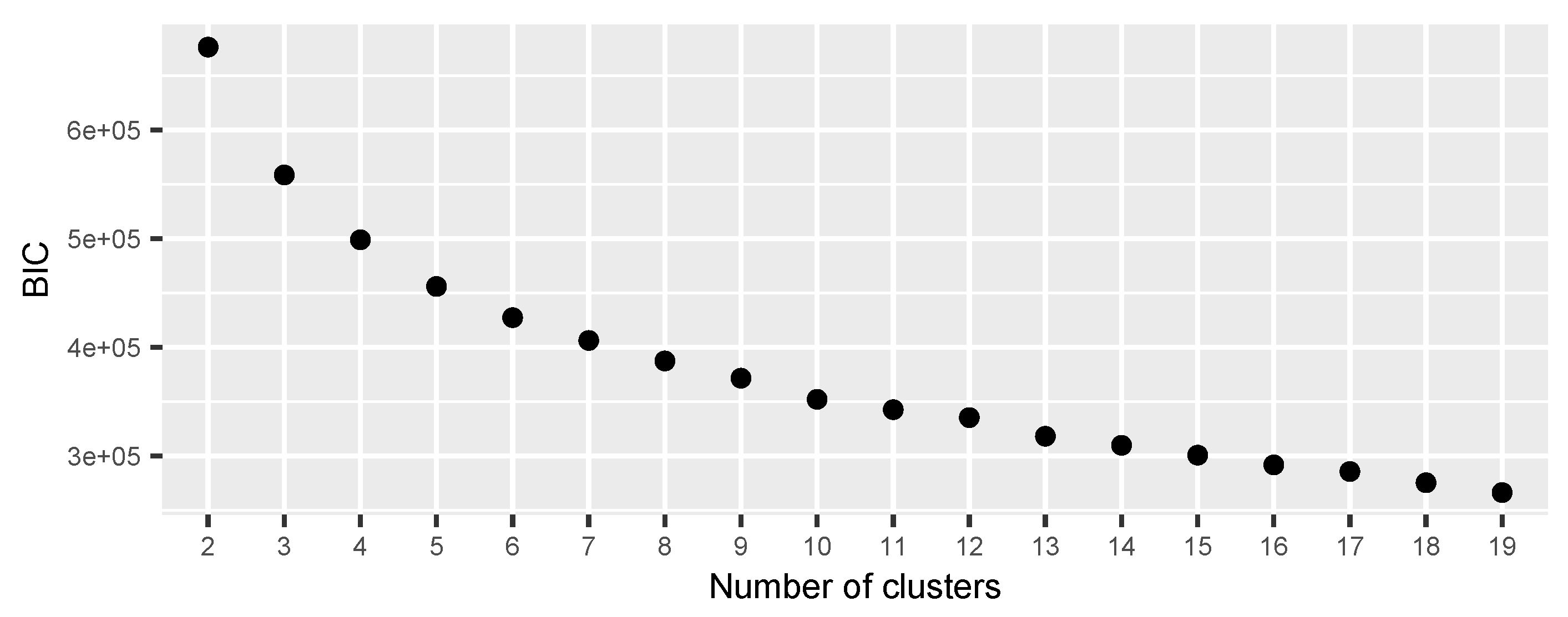

Table A1.
Maximal temperature difference of the inversion layer to a height of 750 m. Only for clusters 10 and 12 were the maximal temperatures observed lower than at 750 m. For other clusters, the temperatures at 750 m are given.
Table A1.
Maximal temperature difference of the inversion layer to a height of 750 m. Only for clusters 10 and 12 were the maximal temperatures observed lower than at 750 m. For other clusters, the temperatures at 750 m are given.
| Cluster | 10 | 12 | 13 | 14 | 15 |
|---|---|---|---|---|---|
| Max. temp. () | 2.4 | 3.8 | 4.0 | 5.8 | 7.0 |

Table A2.
Average slope of the centroids calculated as the average difference in two consecutive temperature measurements. The slope is defined as the average change in temperature every 4.5 m.
Table A2.
Average slope of the centroids calculated as the average difference in two consecutive temperature measurements. The slope is defined as the average change in temperature every 4.5 m.
| Cluster | 1 | 2 | 3 | 4 | 5 | 6 | 7 | 8 | 9 | 10 | 11 | 12 | 13 | 14 | 15 |
|---|---|---|---|---|---|---|---|---|---|---|---|---|---|---|---|
| Mean slope | −0.04 | −0.03 | −0.02 | −0.01 | 0.00 | 0.00 | 0.00 | 0.01 | 0.02 | 0.02 | 0.03 | 0.03 | 0.04 | 0.06 | 0.07 |
References
- Gramsch, E.; Cáceres, D.; Oyola, P.; Reyes, F.; Vásquez, Y.; Rubio, M.; Sánchez, G. Influence of surface and subsidence thermal inversion on PM2. 5 and black carbon concentration. Atmos. Environ. 2014, 98, 290–298. [Google Scholar] [CrossRef]
- Milionis, A.; Davies, T. Associations between atmospheric temperature inversions and vertical wind profiles: A preliminary assessment. Meteorol. Appl. 2002, 9, 223–228. [Google Scholar] [CrossRef]
- Glojek, K.; Močnik, G.; Alas, H.D.C.; Cuesta-Mosquera, A.; Drinovec, L.; Gregorič, A.; Ogrin, M.; Weinhold, K.; Ježek, I.; Müller, T.; et al. The impact of temperature inversions on black carbon and particle mass concentrations in a mountainous area. Atmos. Chem. Phys. 2022, 22, 5577–5601. [Google Scholar] [CrossRef]
- Xu, T.; Song, Y.; Liu, M.; Cai, X.; Zhang, H.; Guo, J.; Zhu, T. Temperature inversions in severe polluted days derived from radiosonde data in North China from 2011 to 2016. Sci. Total Environ. 2019, 647, 1011–1020. [Google Scholar] [CrossRef]
- Kim, K.H.; Kabir, E.; Kabir, S. A review on the human health impact of airborne particulate matter. Environ. Int. 2015, 74, 136–143. [Google Scholar] [CrossRef]
- Cheung, K.; Daher, N.; Kam, W.; Shafer, M.M.; Ning, Z.; Schauer, J.J.; Sioutas, C. Spatial and temporal variation of chemical composition and mass closure of ambient coarse particulate matter (PM10–2.5) in the Los Angeles area. Atmos. Environ. 2011, 45, 2651–2662. [Google Scholar] [CrossRef]
- Ma, Y.; Zhu, Y.; Liu, B.; Li, H.; Jin, S.; Zhang, Y.; Fan, R.; Gong, W. Estimation of the vertical distribution of particle matter (PM 2.5) concentration and its transport flux from lidar measurements based on machine learning algorithms. Atmos. Chem. Phys. 2021, 21, 17003–17016. [Google Scholar] [CrossRef]
- Poberžnik, M.; Štrumbelj, E. The effects of air mass transport, seasonality, and meteorology on pollutant levels at the Iskrba regional background station (1996–2014). Atmos. Environ. 2016, 134, 138–146. [Google Scholar] [CrossRef]
- Wu, W.; Zha, Y.; Zhang, J.; Gao, J.; He, J. A temperature inversion-induced air pollution process as analyzed from Mie LiDAR data. Sci. Total Environ. 2014, 479, 102–108. [Google Scholar] [CrossRef]
- Janhäll, S.; Olofson, K.F.G.; Andersson, P.U.; Pettersson, J.B.; Hallquist, M. Evolution of the urban aerosol during winter temperature inversion episodes. Atmos. Environ. 2006, 40, 5355–5366. [Google Scholar] [CrossRef]
- Liu, B.; Ma, X.; Ma, Y.; Li, H.; Jin, S.; Fan, R.; Gong, W. The relationship between atmospheric boundary layer and temperature inversion layer and their aerosol capture capabilities. Atmos. Res. 2022, 271, 106121. [Google Scholar] [CrossRef]
- Li, H.; Liu, B.; Ma, X.; Ma, Y.; Jin, S.; Fan, R.; Wang, W.; Fang, J.; Zhao, Y.; Gong, W. The Influence of Temperature Inversion on the Vertical Distribution of Aerosols. Remote Sens. 2022, 14, 4428. [Google Scholar] [CrossRef]
- Liu, B.; Ma, Y.; Shi, Y.; Jin, S.; Jin, Y.; Gong, W. The characteristics and sources of the aerosols within the nocturnal residual layer over Wuhan, China. Atmos. Res. 2020, 241, 104959. [Google Scholar] [CrossRef]
- Shao, M.; Xu, X.; Lu, Y.; Dai, Q. Spatio-temporally differentiated impacts of temperature inversion on surface PM2. 5 in eastern China. Sci. Total Environ. 2023, 855, 158785. [Google Scholar] [CrossRef] [PubMed]
- Kikaj, D.; Vaupotič, J.; Chambers, S.D. Identifying persistent temperature inversion events in a subalpine basin using radon-222. Atmos. Meas. Tech. 2019, 12, 4455–4477. [Google Scholar] [CrossRef]
- Yin, P.Y.; Chang, R.I.; Day, R.F.; Lin, Y.C.; Hu, C.Y. Improving PM2. 5 concentration forecast with the identification of temperature inversion. Appl. Sci. 2022, 12, 71. [Google Scholar] [CrossRef]
- Łupikasza, E.B.; Niedźwiedź, T. Relationships between Vertical Temperature Gradients and PM10 Concentrations during Selected Weather Conditions in Upper Silesia (Southern Poland). Atmosphere 2022, 13, 125. [Google Scholar] [CrossRef]
- Huang, Q.; Chu, Y.; Li, Q. Climatology of low-level temperature inversions over China based on high-resolution radiosonde measurements. Theor. Appl. Climatol. 2021, 144, 415–429. [Google Scholar] [CrossRef]
- Bailey, A.; Chase, T.N.; Cassano, J.J.; Noone, D. Changing temperature inversion characteristics in the US Southwest and relationships to large-scale atmospheric circulation. JAMC 2011, 50, 1307–1323. [Google Scholar]
- Li, J.; Chen, H.; Li, Z.; Wang, P.; Cribb, M.; Fan, X. Low-level temperature inversions and their effect on aerosol condensation nuclei concentrations under different large-scale synoptic circulations. Adv. Atmos. Sci. 2015, 32, 898–908. [Google Scholar] [CrossRef]
- Guo, J.; Chen, X.; Su, T.; Liu, L.; Zheng, Y.; Chen, D.; Li, J.; Xu, H.; Lv, Y.; He, B.; et al. The climatology of lower tropospheric temperature inversions in China from radiosonde measurements: Roles of black carbon, local meteorology, and large-scale subsidence. J. Clim. 2020, 33, 9327–9350. [Google Scholar] [CrossRef]
- Kahl, J.D. Characteristics of the low-level temperature inversion along the Alaskan Arctic coast. Int. J. Climatol. 1990, 10, 537–548. [Google Scholar] [CrossRef]
- Milan, M.; Haimberger, L. Predictors and grouping for bias correction of radiosonde temperature observations. J. Geophys. Res. Atmos. 2015, 120, 10–736. [Google Scholar] [CrossRef]
- Kong, D.; Ning, G.; Wang, S.; Cong, J.; Luo, M.; Ni, X.; Ma, M. Clustering diurnal cycles of day-to-day temperature change to understand their impacts on air quality forecasting in mountain-basin areas. Atmos. Chem. Phys. 2021, 21, 14493–14505. [Google Scholar] [CrossRef]
- Truong, S.; Huang, Y.; Lang, F.; Messmer, M.; Simmonds, I.; Siems, S.; Manton, M. A climatology of the marine atmospheric boundary layer over the Southern Ocean from four field campaigns during 2016–2018. J. Geophys. Res. Atmos. 2020, 125, e2020JD033214. [Google Scholar] [CrossRef]
- Govender, P.; Sivakumar, V. Application of k-means and hierarchical clustering techniques for analysis of air pollution: A review (1980–2019). Atmos. Pollut. Res. 2020, 11, 40–56. [Google Scholar] [CrossRef]
- Saeipourdizaj, P.; Musavi, S.; Gholampour, A.; Sarbakhsh, P. Clustering the Concentrations of PM10 and O3: Application of Spatiotemporal Model–Based Clustering. Environ. Model. Assess. 2022, 1–10. [Google Scholar] [CrossRef]
- Nidzgorska-Lencewicz, J.; Czarnecka, M. Thermal inversion and particulate matter concentration in Wrocław in the winter season. Atmosphere 2020, 11, 1351. [Google Scholar] [CrossRef]
- Czarnecka, M.; Nidzgorska-Lencewicz, J.; Rawicki, K. Temporal structure of thermal inversions in Łeba (Poland). Theor. Appl. Climatol. 2019, 136, 1–13. [Google Scholar] [CrossRef]
- Pérez, I.; Sánchez, M.; García, M.; Pardo, N. Boundaries of air mass trajectory clustering: Key points and applications. Int. J. Environ. Sci. Technol. 2017, 14, 653–662. [Google Scholar] [CrossRef]
- Sokolov, A.; Dmitriev, E.; Maksimovich, E.; Delbarre, H.; Augustin, P.; Gengembre, C.; Fourmentin, M.; Locoge, N. Cluster analysis of atmospheric dynamics and pollution transport in a coastal area. Bound. Layer Meteorol. 2016, 161, 237–264. [Google Scholar] [CrossRef]
- Mlakar, P.; Nummi, T.; Oblak, P.; Pucer, J.F. SMIXS: Novel efficient algorithm for non-parametric mixture regression-based clustering. arXiv 2022, arXiv:2209.09030. [Google Scholar]
- Pucer Faganeli, J.; Štrumbelj, E. Impact of changes in climate on air pollution in Slovenia between 2002 and 2017. Environ. Pollut. 2018, 242, 398–406. [Google Scholar] [CrossRef]
- Bec, D.; Ciglenečki, D. P.D.L.M.G.M.K.T.K.M.L.L.M.M.M.M.R.R.Ž. Kakovost zraka v Sloveniji v letu 2021. Technical Report, ARSO. 2021. Available online: https://igs.org/news/igs-technical-report-2021/ (accessed on 1 January 2023).
- Largeron, Y.; Staquet, C. Persistent inversion dynamics and wintertime PM10 air pollution in Alpine valleys. Atmos. Environ. 2016, 135, 92–108. [Google Scholar] [CrossRef]
- Slovenian Environment Agency. 2022. Available online: https://www.arso.gov.si/en/ (accessed on 13 September 2022).
- Golden, J.; Serafin, R.; Lally, V.; Facundo, J. Atmospheric sounding systems. In Mesoscale Meteorology and Forecasting; Springer: Berlin/Heidelberg, Germany, 1986; pp. 50–70. [Google Scholar]
- Prasad, P.; Basha, G.; Ratnam, M.V. Is the atmospheric boundary layer altitude or the strong thermal inversions that control the vertical extent of aerosols? Sci. Total Environ. 2022, 802, 149758. [Google Scholar] [CrossRef]
- Haeger-Eugensson, M.; Holmer, B. Advection caused by the urban heat island circulation as a regulating factor on the nocturnal urban heat island. Int. J. Climatol. J. R. Meteorol. Soc. 1999, 19, 975–988. [Google Scholar] [CrossRef]
- European Council. Directive 2008/50/EC of the European Parliament and of the Council. Decision of Council. 2008. Available online: https://www.consilium.europa.eu/en/european-council/ (accessed on 1 January 2023).
- Nummi, T.; Salonen, J.; Koskinen, L.; Pan, J. A semiparametric mixture regression model for longitudinal data. J. Stat. Theory Pract. 2018, 12, 12–22. [Google Scholar] [CrossRef]
- McLachlan, G.J.; Lee, S.X.; Rathnayake, S.I. Finite mixture models. Annu. Rev. Stat. Its Appl. 2019, 6, 355–378. [Google Scholar] [CrossRef]
- Schwarz, G. Estimating the dimension of a model. Ann. Stat. 1978, 6, 461–464. [Google Scholar] [CrossRef]
- Mlakar, P. The Use of Mixture Regression in Machine Learning. Ph.D. Thesis, Univerza v Ljubljani, Ljubljanatel, Slovenia, 2021. [Google Scholar]
- Lee, S.W.; Kim, S.; Lee, Y.S.; Choi, B.I.; Kang, W.; Oh, Y.K.; Park, S.; Yoo, J.K.; Lee, J.; Lee, S.; et al. Radiation correction and uncertainty evaluation of RS41 temperature sensors by using an upper-air simulator. Atmos. Meas. Tech. 2022, 15, 1107–1121. [Google Scholar] [CrossRef]
- Faganeli Pucer, J.; Pirš, G.; Štrumbelj, E. A Bayesian approach to forecasting daily air-pollutant levels. KAIS 2018, 57, 635–654. [Google Scholar] [CrossRef]
- Niedźwiedź, T.; Łupikasza, E.B.; Małarzewski, Ł.; Budzik, T. Surface-based nocturnal air temperature inversions in southern Poland and their influence on PM10 and PM2.5 concentrations in Upper Silesia. Theor. Appl. Climatol. 2021, 146, 897–919. [Google Scholar] [CrossRef]
Disclaimer/Publisher’s Note: The statements, opinions and data contained in all publications are solely those of the individual author(s) and contributor(s) and not of MDPI and/or the editor(s). MDPI and/or the editor(s) disclaim responsibility for any injury to people or property resulting from any ideas, methods, instructions or products referred to in the content. |
© 2023 by the authors. Licensee MDPI, Basel, Switzerland. This article is an open access article distributed under the terms and conditions of the Creative Commons Attribution (CC BY) license (https://creativecommons.org/licenses/by/4.0/).

