1. Introduction
Energy consumption seems to be increasing at a tremendous rate which influences many countries to turn toward renewable energy sources [
1]. Furthermore, as a result of pollution, depletion of traditional energy sources, ecological harm, the threat of energy shortages, and atmospheric pollution, the globe is increasingly reliant on renewable and clean energy sources such as wind energy [
2]. Naturally, one of the most significant advantages of renewable energy is that a considerable portion of it qualifies as green and clean energy. Machine Learning (ML) applications in the manufacturing fields of renewable energies (wind, solar, bio-mass, and hydro-power), smart grids, the catalysis industry, and power storage and distribution significantly impact sustainability and the environment.
Artificial neural networks are the most recommended method among ML algorithms because they can generalize perfectly [
3]. Predicting wind speeds is essential for both air pollution model concentrations and the production of wind energy. The ability to predict wind speed is essential for reducing the standby cost of the wind power grid and choosing the best reserve capacity at various time intervals [
4]. Machine learning in wind speed predicts produces excellent and dependable power system maneuvers. As a result, the operating costs of producing wind energy were greatly decreased, and the design and construction of power systems and wind farms were aided by the effective integration of wind energy into the electrical power grid.
The author propositions a durable wind speed extrapolation exemplary based on innumerable artificial neural network approaches, including Improved Back-Propagation Network (IBPN), Multi-layer Perception Network (MLPN), Recursive Radial Basis Function Network (RRBFN), and Elman Network, in the study [
5]. Senjyu et al. [
6] suggested utilizing RNN to anticipate wind speed and use that information to prognosticate the output supremacy of wind generators. According to [
7], the author employs an inter-short-term wind speed projection technique that makes use of multivariate exogenous input factors. Conv-LSTM and BPNN models are used by Gonggui et al. to address the issue of wind speed prediction. As the final prediction values, they evaluated the performance assessment matrix (MAPE = 2.62%,
RMSE = 0.151) [
8]. After testing with CEEDMAN (combining full ensemble empirical mode decomposition adaptive noise), flower pollination algorithm with chaotic local search (CLSFPA), five neural networks, and no negative constraint theory (NNCT), Wenyu et al. proposed an appropriate wind speed prediction model [
9]. In this study [
10], a hybrid model for short-term wind speed prediction was suggested. The model is tailored to the wind speed data set and extracts energetic properties to support window slant in speed prediction. Because wind speed displays high intermodulation distortion and features typically, to improve prediction performance [
11]. The suggested system is a revolutionary hybrid prediction system with efficient data decomposition methods, recurrent neural network algorithms, and error deconstruction repair mechanisms. A highly accurate short-term prediction model is required to fill the research gap in wind speed prediction applications. Due to the effect of different atmospheric conditions, the wind is unpredictable.
A trustworthy prediction model is therefore required. The proposed short-term wind speed prediction models in this study solved the research gaps indicated previously by including the essential influencing parameters as model inputs [
12]. The ability to anticipate wind speed is a vital hot issue in the study since it is unpredictable and time-varying. Our proposed study paper makes the following significant contributions:
An appropriate wind speed prediction model is suggested, and among the models, ANN is thought to be the best.
Wind speed prediction concerning short-term horizon.
Analyzed a real-time wind data-set to assess the performance of the suggested models.
Concerning hidden neurons, evaluations based on functionality and consistency were conducted.
Assessment criteria are used to compare actual and predicted data to determine how well the proposed model predicts future wind speed values.
Here, the key elements of the short-term wind speed extrapolation model’s development and performance improvement, which will be covered in greater depth later, are noted. The rest of the article is organized like follows:
Section 2 emphasizes the importance of predicting wind speed.
Section 3 illustrates the related works to this research. The methodology of this research, the development procedure of the model, and the details steps to carry out the outcome of the research are discussed in
Section 4.
Section 5 discusses the performance evaluation metrics.
Section 6 highlights the model’s structural framework. In
Section 7 the ANN model results are reviewed, and identifying the ANN model outcomes is based on the diversity of optimizer functions.
Section 8 provides the future scope of the thesis so that it can be updated in future work, and
Section 9 concludes the paper.
2. Significance of Anticipating Wind Speed
Due to a lack of traditional energy sources, environmental harm, and carbon dioxide emissions, wind speed scheming has been a popular topic in research. Because of various common characteristics, including its self-erudition solid aptitude, real-time maneuverability, fault tolerance, straightforward implementation, and economic viability, ANN is extensively employed in wind speed predicting [
13]. However, wind power has a detrimental effect on the power system because of how abrupt, unpredictable, and indecisive. These adverse consequences have mitigated the significance of predicting the wind speed is explained further beneath:
To support the administration of a wind farm and electricity grid.
Wind energy is really being integrated into the electricity grid.
Jobs in the power system that are constant and critical.
To determine the need for a system with a shorter gyrating fallback.
To reduce the cost at which wind energy is generated.
Time series analysis offers several instruments for weather and climate research, including weather prediction, the development of wind farms, etc. Decentralized methods, such as numerical prediction models, are typically used to estimate wind speed in small time increments [
14]. The goal of this study is to use an artificial neural network to analyze time series data of wind speed at 10-min intervals (ANN). Several other authors have revealed appropriate forms of this paper, including Perez-Llera et al. [
15], Bilgili M et al. [
16], Torres JL et al. [
17], H. Selcuk Nogay et al. [
18], Karakuş O et al. [
19], and Neshat et al. [
20].
3. Related Works
This article has presented a research study related to this research. It is split into two segments. The first portion discusses predicting wind speed, while the second section discusses machine learning techniques. In the second section, both long-term wind speed prediction using machine learning approaches and short-term wind speed prediction using artificial neural networks are covered.
3.1. Prediction of Wind Speed
An instantaneous speed is noted as a peak wind speed, wind gust, or squall; alternatively, it could be an averaged the phrase “wind speed” describes the rate at which air is moving past a specific spot. For a flexible and intelligent electricity grid, wind parameter prediction is essential. By predicting wind parameters, wind power generation can be anticipated. A wind farm can benefit greatly from this in terms of maintenance, planning, and productivity. Wind speed and direction are essential for monitoring and predicting weather patterns and the state of the global climate.
3.2. Wind Speed Prediction Using ML Techniques
A frequent and accurate prediction of wind speed is necessary for wind energy, a renewable energy source with enormous development potential. Using the fireworks approach, an LSTM neural network-based wind speed estimation model was improved (FWA). In an integrated predicting strategy, it is also advised for hyperparameter tuning [
21]. FWA is used to improve the hyperparameters of an LSTM-based wind speed prediction model. The model’s parameters may be established adaptively, highlighting the model’s reliance on wind speed data and rapid real-time change. For short-term time series prediction, Viet et al. [
22] suggests a hybrid deep learning-based architecture termed ConvLSTM. The recommended computational structure conglomerates the advantages of CNN and LSTM networks to produce highly accurate wind speed predictions with fewer hidden neurons, delays, and computing complexity. RNN identify the sequential properties of input and utilize patterns to predict the likely situation that follows. This paper proposes an innovative hybrid prediction system that combines effective data disintegration procedures, recurrent neural network extrapolation systems, and error putrefaction dealings [
23]. The study uses both univariate and multivariate ARIMA models, as well as their recurrent neural network counterparts, to predict wind speed. Recurrent neural network models outperform ARIMA models, whereas multivariate models outperform univariate models, according to the study’s findings [
24]. Finally, it is possible to infer that the use of machine learning algorithms in wind speed prediction is increasing on a daily basis in order to more precisely predict wind speed while also reducing prediction time and cost.
3.2.1. ANN for Long-Term Wind Speed Prediction
Due to the energy crisis, finding marginal energy cradles for a sustainable energy stream has become critical, and wind energy is one of the appealing choices. An essential component of a wind energy scheme is wind speed. Avoid ineffective and less dependable results, wind energy, which has unstable and intermittent features. Long-term wind speed prediction is a popular topic that necessitates the establishment of precise projected data for the best design of wind farms, restructured electricity markets, and energy management are just a few of the research areas.
3.2.2. ANN-Based Short-Term Wind Speed Prediction
The term “short-term wind speed prediction” refers to hourly and daily prediction for the next 24 and 72 h, respectively. In [
24], wind speed data were chosen to see how a space-time model might estimate wind speed. Furthermore, wind speed demonstrates significant non-linearity and non-stationarity. In order to improve prediction accuracy, Duan et al. [
11] suggests a particular hybridized prediction system that combines efficient data putrefaction techniques, recurrent neural network prophecy algorithms, and error fetidness repair methods. Short-term and long-term wind speed prediction, on the other hand, is required for the installation of any wind farm.
Table 1 lists important traits and findings from several studies using long-term and short-term wind speed prediction.
4. Methodology
Even though it is necessary to estimate wind speed owing to the uneven nature of wind, data-driven approaches are often employed to accomplish so [
29]. In most circumstances, wind speed prognosis is difficult, especially when air pollution modeling is included [
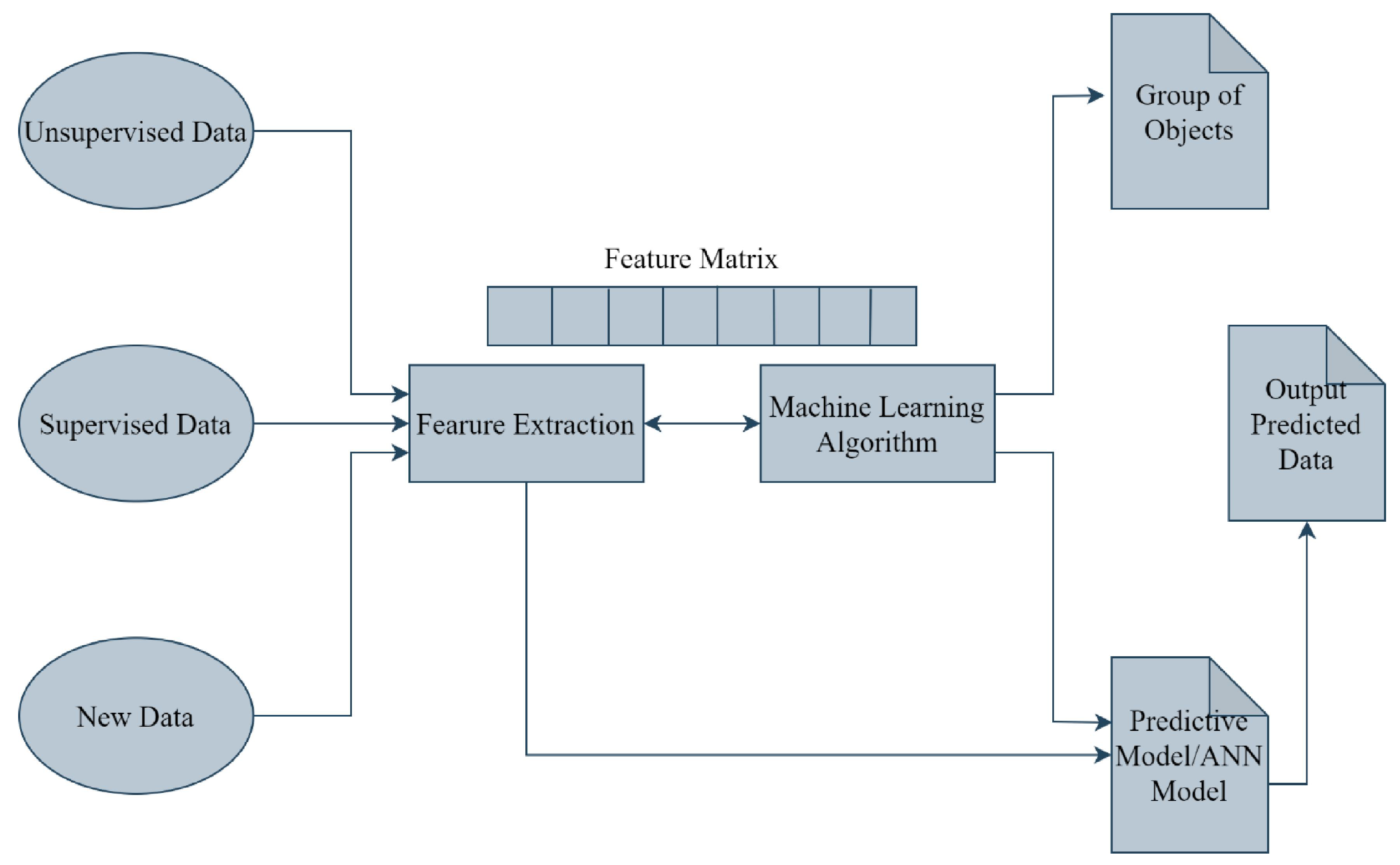
30]. Machine learning techniques can play a tremendous role in data mining approaches, especially in classification and regression problems. Here we are concerned with the regression problem that strongly focuses on predicting future conditions or values of a particular data based on the current state or values of these data. Machine learning automatically completes a specific task by teaching one of its algorithms what to do with a particular data set. The importance of a specific machine learning method in training the data set is seen in
Figure 1 below.
Learning begins with observations or knowledge, such as examples, first-hand experience, or teaching, to seek patterns in the data and subsequently make better decisions based on the examples we provide. The major objective is to make it possible for computers to respond appropriately without human intervention or assistance and to change activities as needed.
4.1. Time Series Forecasting
Prediction is the act of scaling something by one or more user data. A significant field of scholarly investigation into the accumulation of data from time series observations is time series prediction [
31]. A time series will offer predictions of brand-new words in the future, which may be compared to what has already been seen. Suppose we predict time series
,
,……
and the future value
where h is the lead time. The prediction method is an algorithmic rule and procedure used in the predicting model to anticipate future data based on the current or present observed data. There are several prediction methods, such as Judgemental, Univariate, and Multivariate time series prediction.
Here, we focus only on multivariate prediction based on the types of dataset features. To anticipate a multivariate time series, more than one feature, or more than one equation, must be included if the components are interdependent. Techniques for analyzing time series data are used to provide beneficial statistical results that reveal the data’s many properties. By using a model to estimate future values using previously observed information, time series prediction is a technique. With training and testing data taken from Turkey’s online SCADA system, the research uses machine learning.
4.2. Model Overview (ANN)
The artificial neural network is a framework for data processing that is used to examine many aspects of a system that processes information and is prompted by the human nervous system, such as the brain [
32]. The connectionist model of the neural network is used to train and recall algorithms, and this connection forms the neural structure of the network [
33]. The usage of ANN is widespread due to its many advantages, including its high level of flexibility, self-learning capacity, and error tolerance. Elman, Hopfield, and Boltzmann machines are examples of feedback networks [
34].
Networks that transmit information forward and backward are known as artificial neural networks (ANN). Feed-forward networks have input-to-output layers like MLP, BPN, and RBFN, for example [
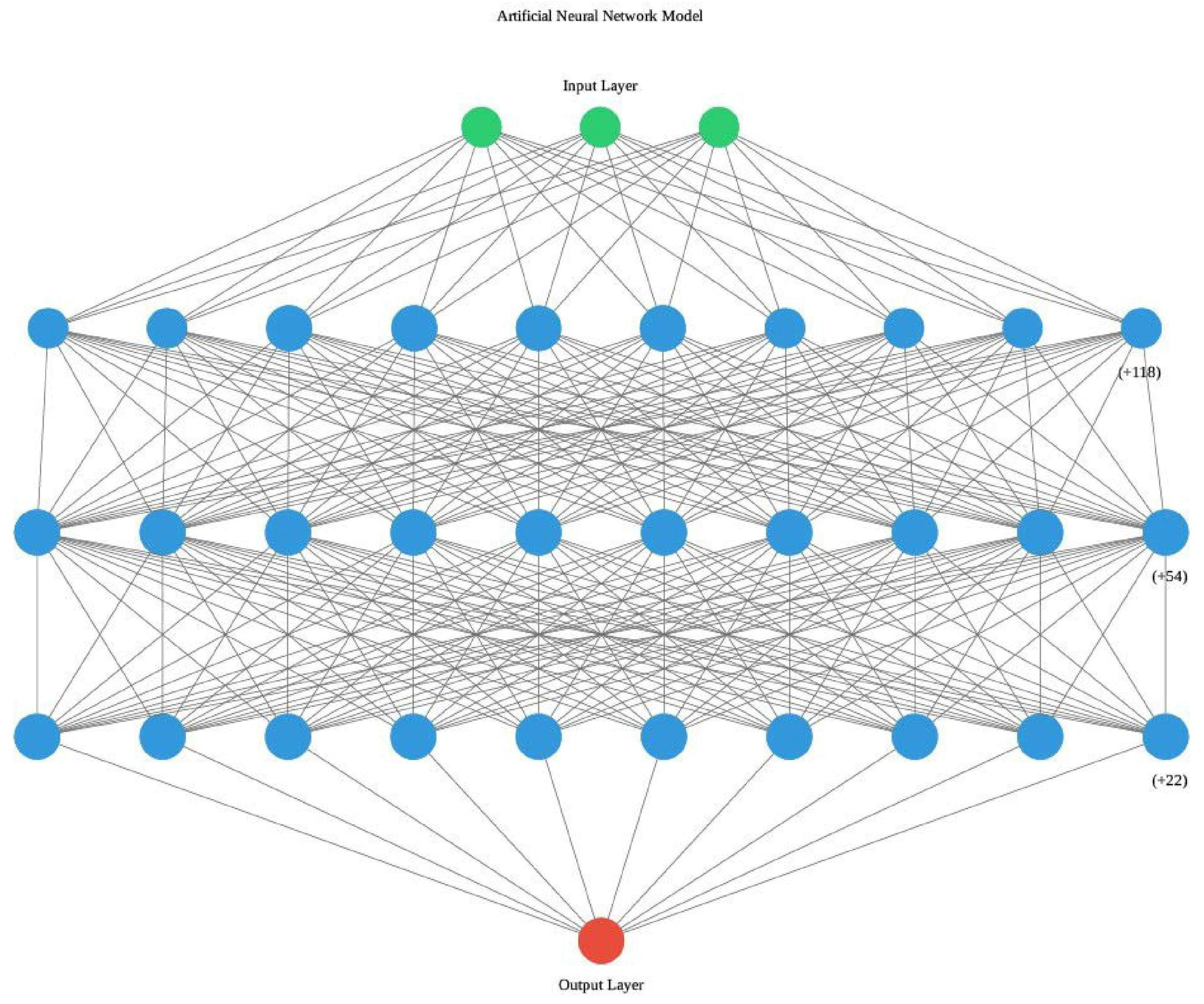
35]. The suggested wind speed prognosis model is built with four inputs, and the optional input is omitted from the data set, which has no effect on the wind speed prediction. This model’s input and output vectors are explained below:
Input vector X = [Wind speed (m/s), LV active power (kW), Wind direction (degree), Theoretical power curve (Kwh)].
Output vector Y = [predicted wind speed (m/s)].
The ANN model’s architecture is ultimately linked, with three concealed layers and one yield layer. The architecture of the ANN-based short-term wind speed prediction model is depicted in
Figure 2.
The weights are multiplied by the inputs in the feed-forward process, and the resulting value is stimulated toward the ensuing layer until it approaches the production layer, as shown below [
36]:
Here,
and
are activation functions, and
is the weight relocated from the
jth input to the
ith node, which is the input
is the synopsis of inputs of the
ith node. Using trial and error methods together with the necessary information, the correct number of neurons in the hidden layer and the transfer functions are established. The back-propagation approach yields the error value by computing the difference between the anticipated and expected values, starting with an output layer and working your way back to the input layer. It is signposted by the representation
, which correspondent to the blunder of node
j in layer
l.
After adjusting the weight, the technique is done multiple times because it is monotonous. When the model is processed, the remembered weights are kept in the ANN. The amount of DoF (degree of freedom) required to fully master the processing operation and how long it takes to complete the processing operation are both strongly influenced by the number of input and output nodes. As the amount of hidden nodes grows, the system may occasionally become overly well-fitted [
37]. The ANN execution is examined when training is complete. Depending on the outcome, the ANN may need to be retrained or may very well be used for the intended purpose.
4.3. Data Collection
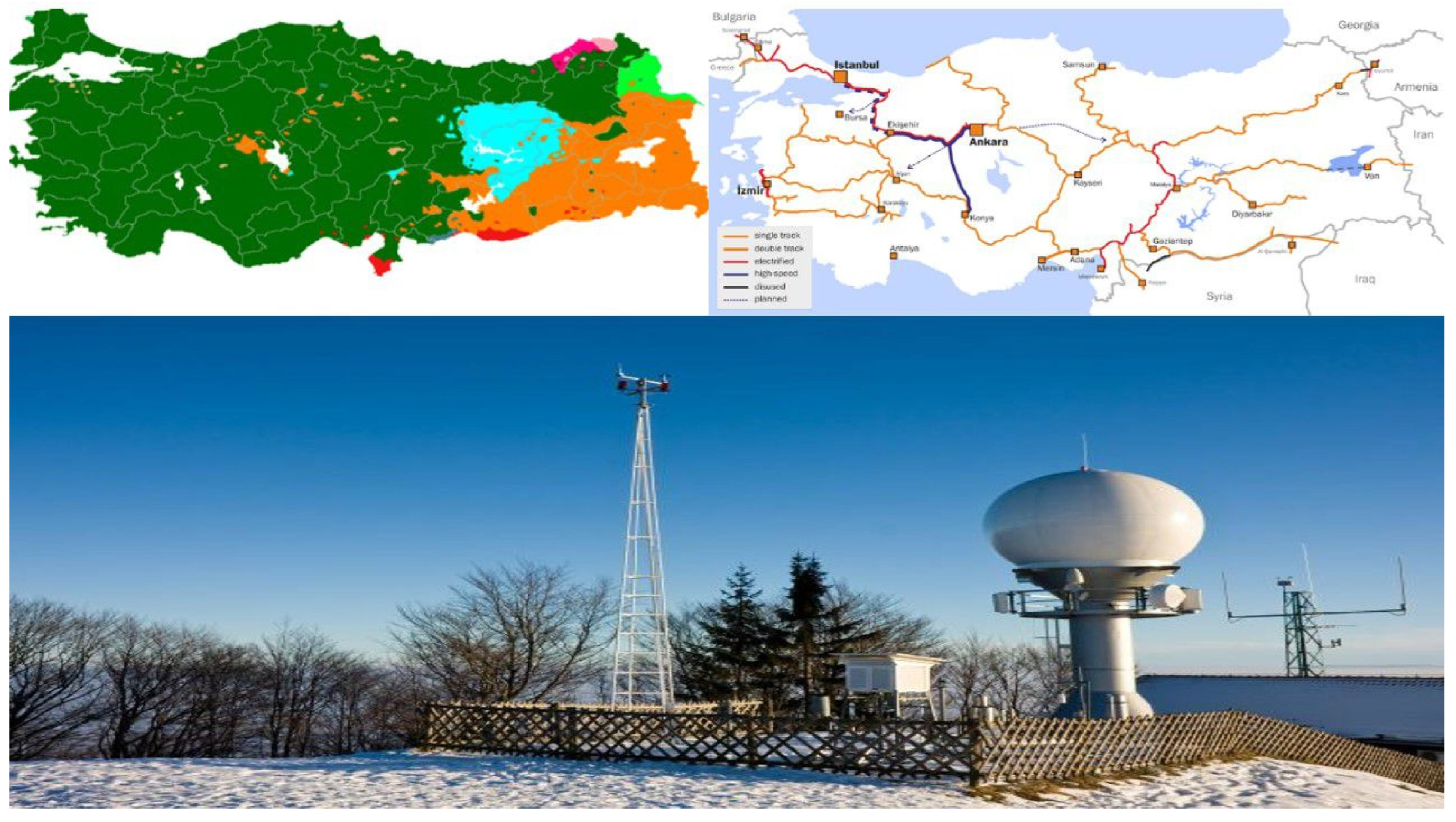
Data from a wind turbine’s SCADA system that was operational and producing power in Turkey from January to December 2018 was gathered for this study. SCADA Systems measure and store information in wind turbines every ten minutes, including wind speed, wind direction, generated electricity, and other factors [
38]. The data monitoring system and meteorological stations are displayed in
Figure 3. This stage is crucial since how effective your prediction model may be will genuinely depend on the type and volume of data we gather. The research’s data set includes the following:
Date/Time (for 10 min interludes)
LV Active Power (kW): The turbine’s output at the moment in terms of power.
Wind Speed (m/s): At the height of the turbine’s hub, the wind speed.
Theoretical Power Curve (KWh): The turbine’s theoretical power outputs at the wind speed recommended by the manufacturer.
Wind Direction (°): The wind direction at the turbine’s hub height.
4.4. Data Preparation
We load our data in the proper location and prepare it for usage in our machine learning model training. Additionally, this would be a good time to perform any necessary visualizations of our data to assist us to identify any imbalances and determine whether there are any relevant connections between different elements that we can take advantage of. In the beginning, there were 52,530 rows in the data-set obtained from the SCADA system archive in Turkey. The data-set will be split into two parts for our analysis. The initial segment will comprise the majority of the data set needed to build the model. The training set contains the vast bulk of the data (75%). The second data-set component will be utilized to test the model. Roughly 25% of the original data set is present in the testing data set. The data we acquire occasionally requires various kinds of modifications and alterations. During this phase, tasks including standardization, error correction, the elimination of certain columns or features, and more are completed. Depending on the model we choose, we must normalize our data.
4.5. Data-Set Cleaning and Visualization
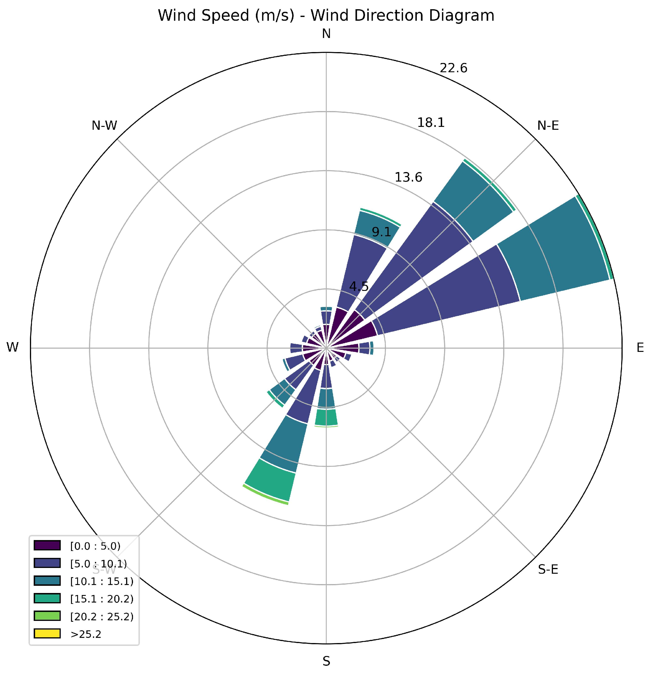
The dataset was collected from the SCADA system in turkey and converted into comma-separated values (CSV). The data will be stored in the data frame and the “Date/Time” features drop out. The data with NaN values will be dropped out from the data frame. The date column will be used to group all of the CSV files, and the mean will then be computed. A CSV file will be used to store the finished data frame. The resultant data will be visualized for further analyzing the dataset.
Figure 4 depicts the wind speed density and rotational angle of the wind turbine rotor with regard to the hub. The wind rose is divided into eight parts, each of which is worth
. The velocity is positioned radially to highlight the wind speed at the specific angle of the turbine rotor. The spoke’s end represents the highest values, while its center represents the lowest, and the incremental velocity is 5 m/s. This figure visualizes that, at the locations of N to E or
–
and S to S-W or
–
of the wind turbine rotor, the wind speed is excessively greater. The varied color-coated rectangles show the velocity range for each co-ordination. The maximum power for high density of wind speed is generated by the rotor positions at
–
degrees and
–
degrees.
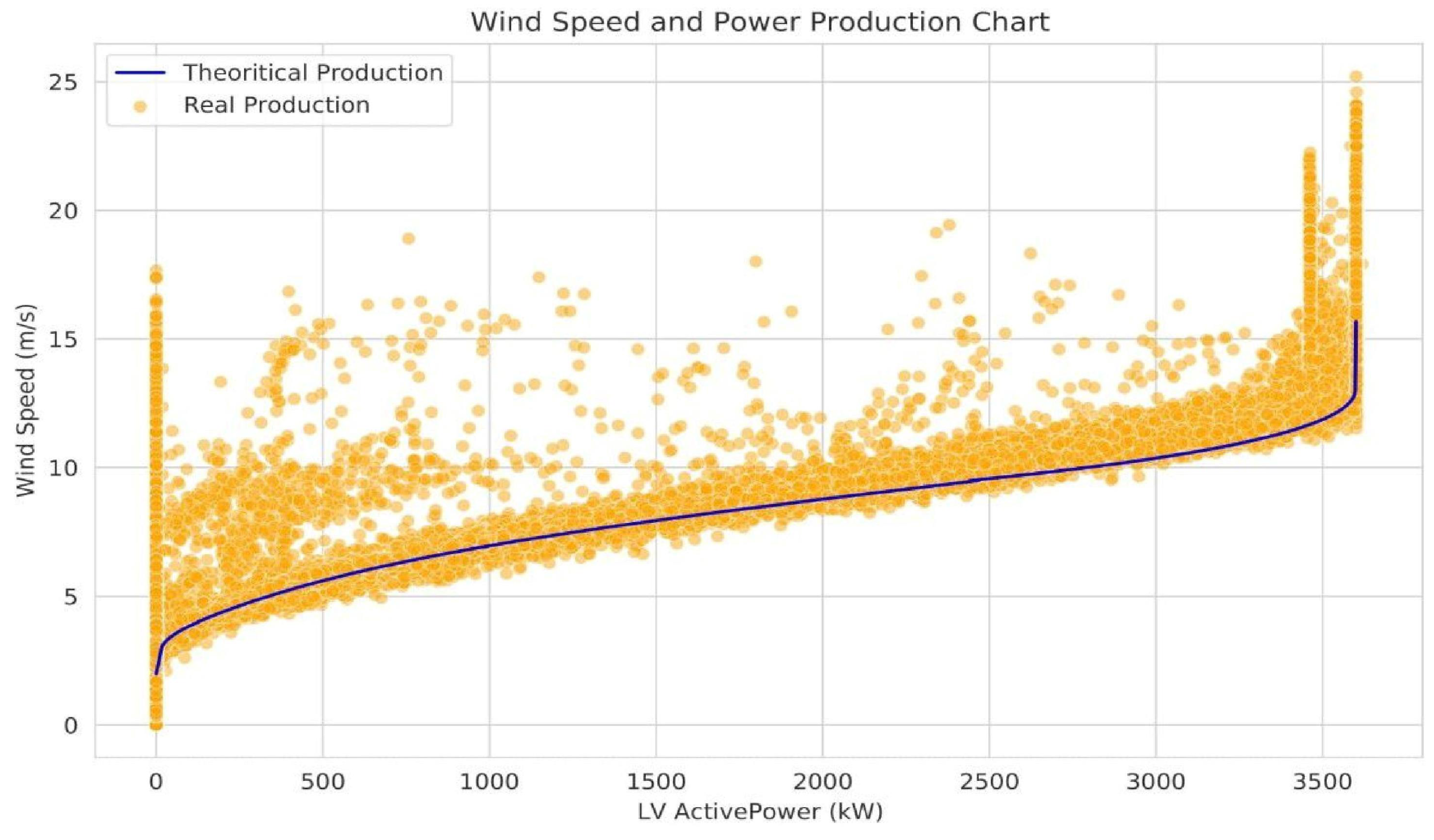
From
Figure 5, we can see that the theoretical power production curve fits well with the real power production (LV Active Power (KW)). This figure also depicts that the wind speed reaches a maximum level and continues in a straight line if the power reaches 3500 KW.
5. Model Performance Evaluation
The main features of regression issues concentrate on simply containing the dataset of the intended actual values, and the errors show how the model makes errors in its prediction. Using specific metrics to make a comparison between the original aim and the predicted one is the primary idea behind assessing the success of the regression model. Depending on the sort of model, different assessment measures are used. We’ll briefly go through the assessment measures in this part to make it easier to see how accurate the regression model is.
5.1. Background in Mathematics
In the succeeding procedures, is the prophesied ith rate, and is the predicted ith value of the elementary SCADA system dataset. The model predicts the value based on the tangible value of dataset , and m is the aggregate data.
5.1.1. Mean Squared Error (MSE)
MSE (Mean Squared Error) is a measure of the difference between actual and expected values that is calculated by squaring the mean difference across the whole data set.
MSE may be used to find any outliers that are required [
40]. The squaring portion of the function enlarges the error if the model eventually produces one especially poor predict.
MSE has the best value of zero and the worst value of (Infinity). The formula for mean squared error is given below:
5.1.2. Root Mean Squared Error (RMSE)
The root mean squared error, or
RMSE, is the calculation’s root (
MSE). The most typical statistic used to judge how well a regression model operates is
RMSE [
41]. The result is that a high
RMSE is “bad” and a low
RMSE is “good”. The formula of
RMSE is shown below:
MSE seems to be the average of the squared residual terms. Additionally, the RMSE is only regarded as the mean squared error’s root (MSE).
5.1.3. Co-Efficient of Determination (R-Squared or )
The strong relationship between the residuals is provided by the coefficient of determination, commonly abbreviated as
(i.e., between the actual and predicted values) [
42]. It spans from 0.0 to 1.0, for instance,
= 0.89 means that
accounts for
of the variance of the anticipated variables in the total observed responses of the data. Here is the simple formula for
given below:
While both
RMSE and
assess a model’s quality of fit, they define ”good” differently. “Good” for
RMSE denotes that the model produces precise predictions (small residuals). “Good” for
signifies that the predictor variable predicts, as opposed to the response variable just having low variation and being straightforward to predict even in the absence of the predictor variable [
43]. There are mainly four conditions taken into consideration for regression models evaluation metrics such as:
Low RMSE and High : The residuals are firmly centered about zero concerning the scale of the response parameters, resulting in why this is regarded as the best situation.
Low RMSE and Low : The models are good enough because the RMSE value is low but the observed values are independent of the predicted values that indirectly highlight no relation in the residuals.
High RMSE and High : In this case, the model produces poor predictions and there is still hope though the predictor determines the observed data.
High RMSE and High (worst case): This is considered the worst case because the model generates crummy predictions (as high RMSE) and the predictor provides no information about the observed data.
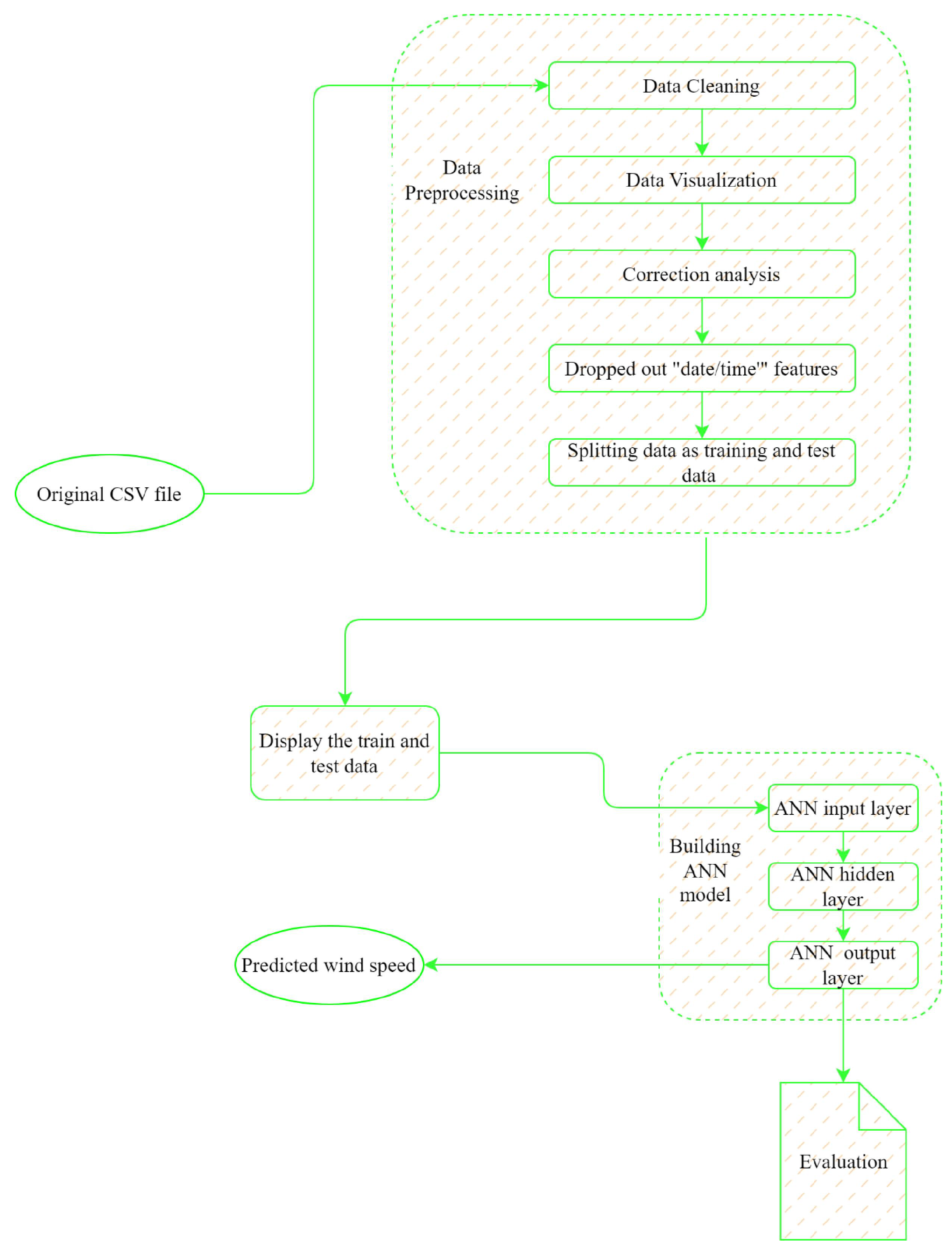
6. The Structure of the ANN-Based Prediction Model for Short-Term Data
The suggested ANN-based model for predicting short-term wind speeds is shown in
Figure 6 as an architectural diagram. A two-part primary model is presented here, with the first section focusing on data preparation and the second highlighting the development of the suggested model. After completing a number of tasks, such as data cleaning and removing extraneous characteristics from the data, the preprocessing portion divides test and train data. The data obtained is then entered into the model to provide the desired result of anticipating future values.
7. Analyze the Results & Discussion
Using a multivariate artificial neural network model, we evaluated the precision of wind speed prediction in this study. So we divided our dataset into training and testing parts, utilizing 25% of the data for testing and the lingering 75% for training. The decision to allocate 75% of the dataset for training and 25% for testing serves a pivotal role in achieving a robust and effective machine learning model. This proportion strikes a delicate equilibrium between two fundamental objectives: nurturing the model’s capacity to comprehend intricate data patterns and validating its proficiency on unseen instances. By dedicating a substantial portion to training, the model is endowed with ample exposure to the underlying relationships within the data, enabling it to discern complex correlations and trends. This mitigates the risk of overfitting, where the model becomes excessively tailored to the training data’s idiosyncrasies. On the other hand, setting aside a quarter of the data for testing facilitates a comprehensive evaluation of the model’s generalization prowess. This reserved subset acts as a litmus test for assessing how well the model extrapolates its learned knowledge to previously unseen scenarios. Ultimately, the 75–25% split encapsulates a well-considered balance that fosters accurate learning while ensuring reliable performance appraisal, laying the foundation for a dependable and insightful machine learning solution.Initially, we build a regressor object with the names and , where has all characteristics except for the one that needs to be predicted and contains those features. The values of the are then predicted.
7.1. The Configuration of Our Proposed ANN Model
The effective Adam optimizer function and the Mean Squared Error (
MSE) loss function were employed. With a batch size of 32, the model will be suitable for 100 training epochs. We can make predictions for the complete test dataset after the model has been fitted. The architecture of a neural network consists of layers, each containing neurons. The choice of the number of layers and neurons in those layers can have a significant impact on the network’s performance. However, there is no one-size-fits-all answer, and the optimal architecture can vary greatly depending on the complexity of the problem, the amount of available data, and other factors. Generally, deeper networks (more layers) can capture complex relationships in the data, but they can also lead to overfitting if not properly regularized. Shallower networks might generalize better but might struggle to learn intricate patterns. Similarly, more neurons per layer can increase the capacity of the network to capture complex patterns, but too many neurons can lead to overfitting. This study layers are more to understand better relationship of the data. The setup of our suggested ANN model, which is utilized to predict the future value of the data, is shown in
Table 2.
7.2. The ANN Model’S Outcome
Table 3 shows that the ANN model has strong prediction outcomes and accuracy due to its low
RMSE and high
value as compare to other methods of study [
44] which used random forest and study [
45] which used neural network for prediction without optimization. This model uses adam optimizer function because of providing the highest performance or co-efficient of performance, and
MSE and
RMSE value among other optimizer functions.
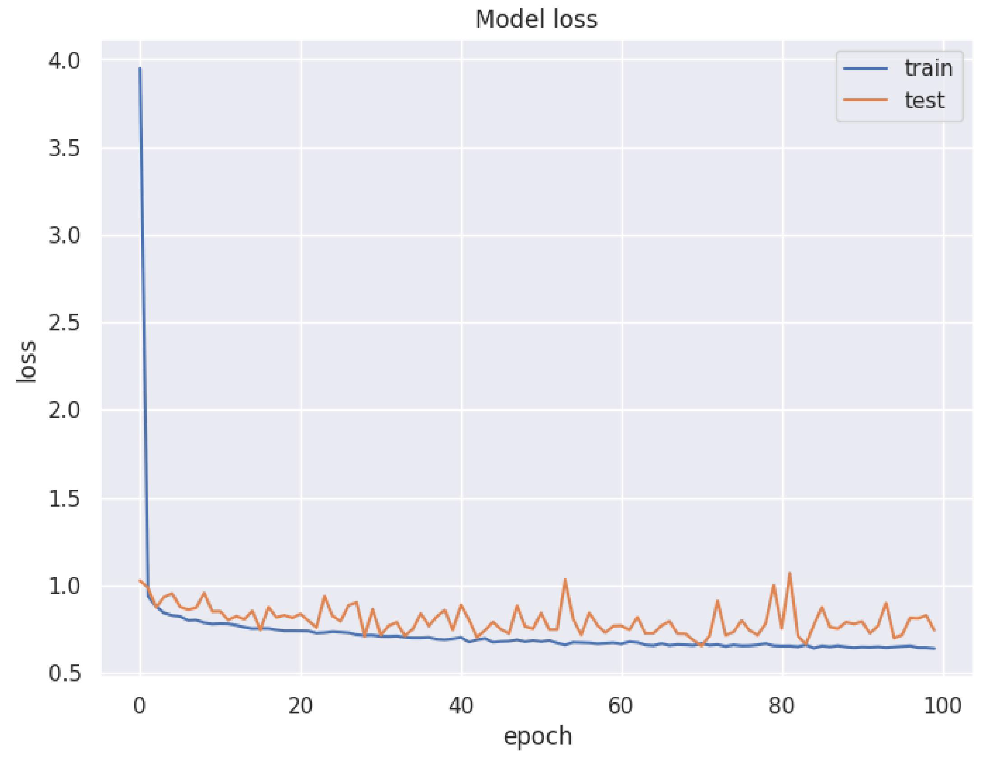
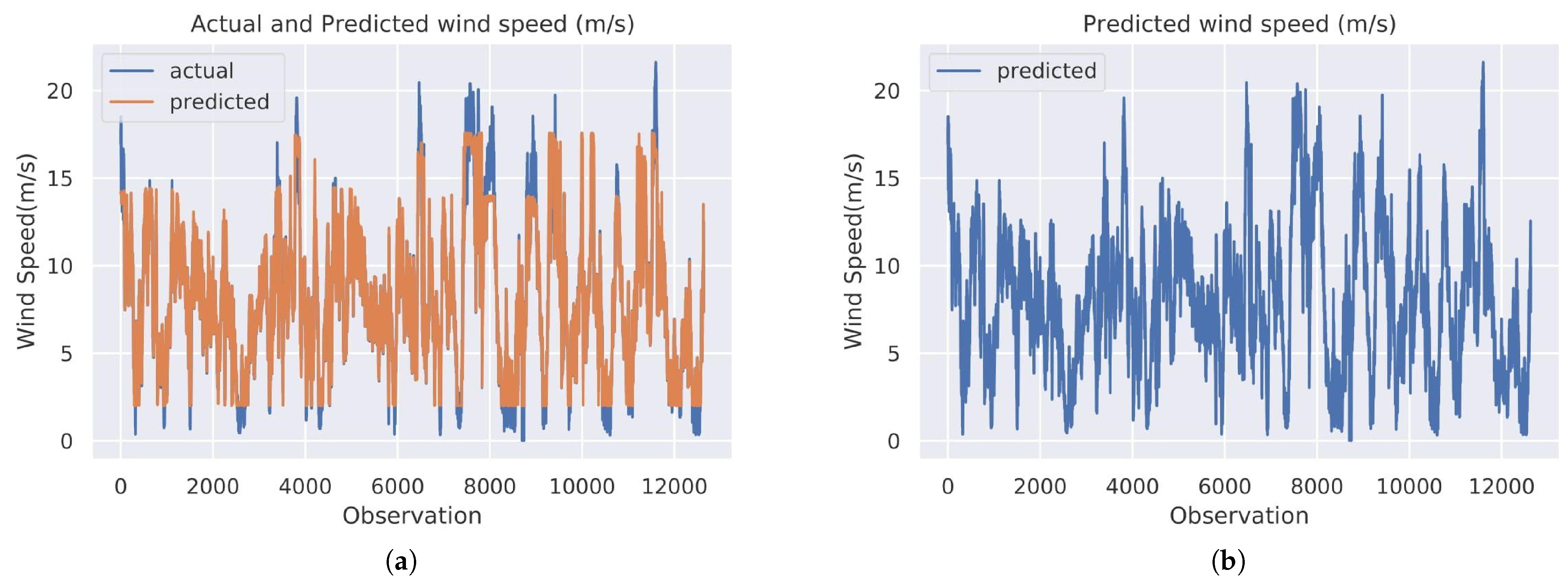
Figure 7. illustrates the training and test error that happens when the model is run on split data. According to this graph, the test error varies between epochs whereas the training error decreases as the number of epochs increases. The discrepancy between the actual and predicted wind speed is shown in
Figure 8a based on the suggested short-term artificial neural network model. More than 12,000 data points of actual and anticipated values are presented for the simplification of
Figure 8a. And
Figure 8b highlights the predicted wind speed of over 25% of test data among the total data of the data-set. The maximum speed of wind exceeds more than 20 m/s and most wind speeds vary from 5 m/s to 15 m/s. When the performance of the suggested model is evaluated using real wind speed-based data, as shown in
Figure 8a, the predicted value is noticeably closer to the actual value. Two estimated metrics, such as
RMSE and
, are regarded critical aspects in evaluating the model’s performance, where the
RMSE value is substantially lower and
is relatively high (from
Table 3), indicating the best scenario among the other four points in the regression model. The ANN model utilized two hundred twenty-five neurons to mend short-term wind speed speculating. The findings support the hypothesis that the suggested method yields superior outcomes over alternatives.
7.3. Statistical Model Evaluation
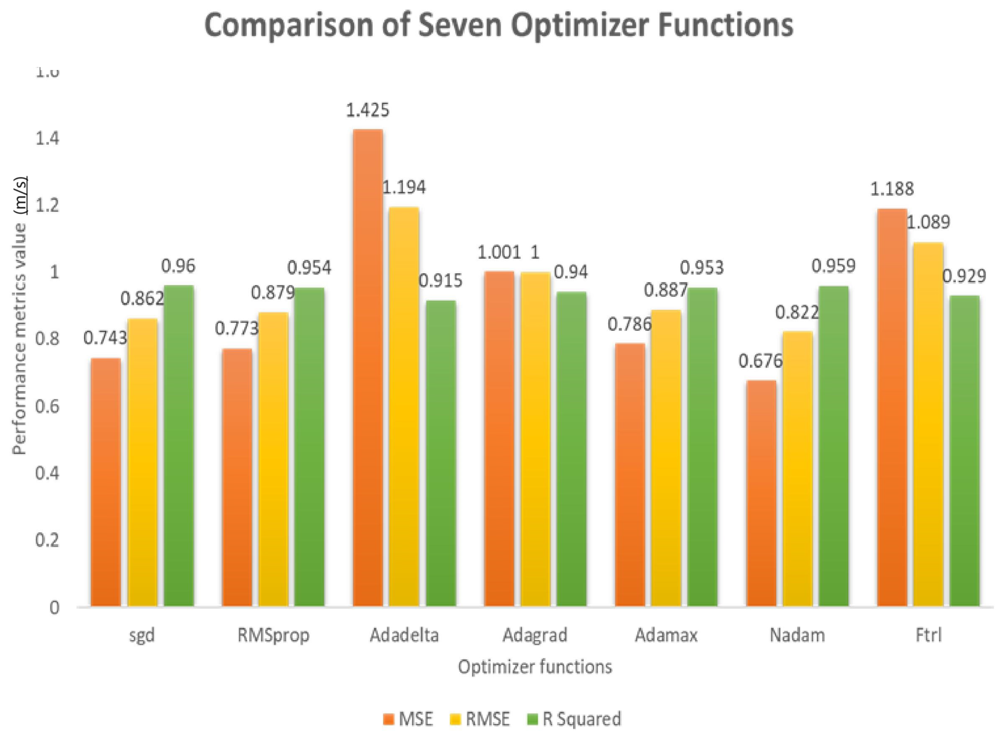
Table 4 illustrates the performance of the model based on different optimizer functions while the neuron numbers are kept the same for all assessment processes.
Figure 9 illustrates the comparison of different optimizers of our proposed ANN model. Suppose, the “Nadam” optimizer highlights the lowest difference between actual and anticipated values than other ones. However, “Adadelta” and “Ftrl” give the greatest discrepancy between the data-actual set’s and projected values. The performance of the model is good for the “sgd” optimizer and bad for the “Adadelta” optimizer as well due to having high and low values of
in comparison to other functions.
8. Future Scope
For easy model training, our model is currently fitted for multivariate parameters. Later, it may be expanded to include various parameters whose data is available in our data-set. On a minute basis, the time series data may be processed with more control over the calculations. Consequently, a more in-depth analysis of the time series data is provided. We may implement Support Vector Regression using the SVM execution developed for this job with the right understanding of the science behind it. Recently, many new methods exists for prediction and deep analysis which can be used for improving results of deep analysis [
46,
47].
While also taking into account changes to the neural network’s engineering, various pre-processing techniques, and the inclusion of new, unique elements, we anticipate keeping an eye out for ways to improve our model’s predictions [
48,
49]. In the future, we’ll take additional measurements to predict working conditions under increasingly severe situations. Additionally, we will consider the fundamental causes of deficits and investigate their characteristics using several time series regression and classification techniques, such as the one that makes use of deep belief networks. Future research will focus on designing a memory block that is more successful, taking into account the drawback of a long training cycle and also developing improved modeling approach [
50,
51,
52].
The presented study holds significant practical implications within the realm of renewable energy, particularly wind energy generation. Given the escalating global focus on mitigating greenhouse gas emissions and transitioning away from fossil fuels, the resurgence of interest in renewable energy sources, like wind energy, becomes highly relevant. Wind power generation has emerged as a leading contender in this transition due to its rapid growth and reputation as a clean energy alternative.
The study’s reliance on real-world data acquired from Turkey’s SCADA system, with 10-min interval measurements, ensures its applicability to practical wind power facilities. This empirical validation underscores the reliability of the proposed approach. The integration of an ANN algorithm, tailored for time series data prediction, enhances the accuracy of short-term wind speed estimations, thereby contributing to more effective resource allocation and operational planning for wind energy facilities.
The reported performance metrics, such as the Mean Squared Error (MSE), Root Mean Squared Error (RMSE), and Coefficient of Determination (R-squared), further substantiate the effectiveness of the ANN algorithm. The study’s notable outcomes, including an MSE of 0.693, an RMSE of 0.833, and an R-squared of 0.96, underscore the model’s ability to provide reliable wind speed predictions.
Practically, these findings hold immense potential for the renewable energy sector. By harnessing accurate short-term wind speed estimations, wind power-producing facilities can optimize energy production, improve grid integration, and enhance overall operational efficiency. Such advancements contribute not only to meeting clean energy targets but also to driving economic and environmental sustainability in the broader context of renewable energy adoption. Due to the reduction of the model’s contribution, it has broad applicability to several grouping display tasks, including content analysis, music identification, and speech recognition. It may also be successfully delivered to continuous frameworks or inserted frameworks due to its small size and productivity. It will need further investigation to determine why the Attention ANN cell fails to successfully coordinate the execution of the General ANN cell on some data-sets.
9. Conclusions
The ability to reduce conventional energy usage and emissions, both of which are viewed as crucial factors in the current environment, makes wind speed prediction essential for renewable energy dispatching. The efficiency of wind energy might be greatly increased by accurate wind speed predictions.
This research plans and investigates strategies for predicting wind speed using short-term wind speed predictions. This study suggests the two-stage disintegration approach combined with short-term wind speed anticipating. The prediction system comprises data preparation, optimization, and deep learning prediction strategies.
This model aids in the prediction of data every ten minutes. Here, the model’s performance may significantly improve wind energy efficiency. RMSE, MSE, and metrics are recycled to prognoses the imminent value of wind speed accurately. In this instance, data from the Turkish SCADA system are utilized, and the dataset is considered for training and testing purposes to validate the performance of the model. Exogenous parameters such as wind direction, LV active power, and theoretical power curve are plausible approaches for calculating short-term wind speed. The MSE, RMSE, and values indicate how effectively the model predicts the wind speed value in the future.
Author Contributions
Methodology, R.K.R., R.A., Z.T., S.H.A., U.A.B., S.K.S., Q.u.A. and Y.Y.G.; Software, R.A., Z.T., S.K.S. and Y.Y.G.; Validation, R.K.R. and S.H.A.; Formal analysis, R.K.R., Z.T., S.H.A., S.K.S. and Q.u.A.; Investigation, R.K.R. and Q.u.A. All authors have read and agreed to the published version of the manuscript.
Funding
This research received no external funding.
Institutional Review Board Statement
Not applicable.
Informed Consent Statement
Not applicable.
Data Availability Statement
Data “available on request”, i.e., all codes and data used in this research will be available by emailing the corresponding author of this research article.
Conflicts of Interest
The authors declare no conflict of interest.
References
- Sun, S.; Liu, Y.; Li, Q.; Wang, T.; Chu, F. Short-term multi-step wind power forecasting based on spatio-temporal correlations and transformer neural networks. Energy Convers. Manag. 2023, 283, 116916. [Google Scholar] [CrossRef]
- Chen, J.; Liu, Z.; Yin, Z.; Liu, X.; Li, X.; Yin, L.; Zheng, W. Predict the effect of meteorological factors on haze using BP neural network. Urban Clim. 2023, 51, 101630. [Google Scholar] [CrossRef]
- Shao, B.; Song, D.; Bian, G.; Zhao, Y. Wind Speed Forecast Based on the LSTM Neural Network Optimized by the Firework Algorithm. Adv. Mater. Sci. Eng. 2021, 2021, 4874757. [Google Scholar] [CrossRef]
- Li, M.; Yang, M.; Yu, Y.; Lee, W. A wind speed correction method based on modified hidden Markov model for enhancing wind power forecast. IEEE Trans. Ind. Appl. 2021, 58, 656–666. [Google Scholar] [CrossRef]
- Madhiarasan, M. Long-term wind speed prediction using artificial neural network-based approaches. Aims Geosci. 2021, 7, 542–552. [Google Scholar] [CrossRef]
- Senjyu, T.; Yona, A.; Urasaki, N.; Funabashi, T. Application of recurrent neural network to long-term-ahead generating power forecasting for the wind power generator. In Proceedings of the 2006 IEEE PES Power Systems Conference and Exposition, Atlanta, GA, USA, 29 October–1 November 2006; pp. 1260–1265. [Google Scholar]
- Noman, F.; Alkawsi, G.; Alkahtani, A.A.; Al-Shetwi, A.Q.; Tiong, S.K.; Alalwan, N.; Ekanayake, J.; Alzahrani, A.I. Multistep short-term wind speed prediction using a nonlinear auto-regressive neural network with exogenous variable selection. Alex. Eng. J. 2021, 60, 1221–1229. [Google Scholar] [CrossRef]
- Chen, G.; Li, L.; Zhang, Z.; Li, S. Short-term wind speed forecasting with principle-subordinate predictor based on Conv-LSTM and improved BPNN. IEEE Access 2020, 8, 67955–67973. [Google Scholar] [CrossRef]
- Zhang, W.; Qu, Z.; Zhang, K.; Mao, W.; Ma, Y.; Fan, X. A combined model based on CEEMDAN and modified flower pollination algorithm for wind speed forecasting. Energy Convers. Manag. 2017, 136, 439–451. [Google Scholar] [CrossRef]
- Hu, J.; Wang, J.; Xiao, L. A hybrid approach based on the Gaussian process with t-observation model for short-term wind speed forecasts. Renew. Energy 2017, 114, 670–685. [Google Scholar] [CrossRef]
- Duan, J.; Zuo, H.; Bai, Y.; Duan, J.; Chang, M.; Chen, B. Short-term wind speed forecasting using recurrent neural networks with error correction. Energy 2021, 217, 119397. [Google Scholar] [CrossRef]
- Duran, M.; Baúaran Filik, Ü. Short-term wind speed prediction using several artificial neural network approaches in Eskisehir. In Proceedings of the International Symposium on Innovations in Intelligent Systems and Applications (INISTA), Madrid, Spain, 2–4 September 2015. [Google Scholar]
- Madhiarasan, M.; Deepa, S.N. New criteria for estimating the hidden layer neuron numbers for recursive radial basis function networks and its application in wind speed forecasting. Asian. J. Inf. Technol. 2016, 15, 4377–4391. [Google Scholar]
- Madhiarasan, M. Accurate prediction of different forecast horizons wind speed using a recursive radial basis function neural network. Prot. Control. Mod. Power. Syst. 2020, 5, 22. [Google Scholar] [CrossRef]
- Perez-Llera, C.; Fernandez-Baizan, M.C.; Feito, J.L.; González del Valle, V. Local Short-Term Prediction of Wind Speed: A Neural Network Analysis. 2002. Available online: https://scholarsarchive.byu.edu/cgi/viewcontent.cgi?article=3693&context=iemssconference (accessed on 12 July 2023).
- Bilgili, M.; Sahin, B.; Yasar, A. Application of artificial neural networks for the wind speed prediction of target station using reference stations data. Renew. Energy 2007, 32, 2350–2360. [Google Scholar] [CrossRef]
- Torres, J.L.; Garcia, A.; De Blas, M.; De Francisco, A. Forecast of hourly average wind speed with ARMA models in Navarre (Spain). Sol. Energy 2005, 79, 65–77. [Google Scholar] [CrossRef]
- Selcuk Nogay, H.; Akinci, T.C.; Eidukeviciute, M. Application of artificial neural networks for short term wind speed forecasting in Mardin, Turkey. J. Energy South. Afr. 2012, 23, 2–7. [Google Scholar] [CrossRef]
- Karakuş, O.; Kuruoğlu, E.E.; Altınkaya, M.A. One-day ahead wind speed/power prediction based on polynomial autoregressive model. IET Renew. Power Gener. 2017, 11, 1430–1439. [Google Scholar] [CrossRef]
- Neshat, M.; Nezhad, M.M.; Abbasnejad, E.; Mirjalili, S.; Tjernberg, L.B.; Garcia, D.A.; Alexander, B.; Wagner, M. A deep learning-based evolutionary model for short-term wind speed forecasting: A case study of the Lillgrund offshore wind farm. Energy Convers. Manag. 2021, 236, 114002. [Google Scholar] [CrossRef]
- Wei, H.; Wang, W.S.; Kao, X.X. A novel approach to ultra-short-term wind power prediction based on feature engineering and informer. Energy Rep. 2023, 9, 1236–1250. [Google Scholar] [CrossRef]
- Viet, D.T.; Phuong, V.V.; Duong, M.Q.; Tran, Q.T. Models for short-term wind power forecasting based on improved artificial neural network using particle swarm optimization and genetic algorithms. Energies 2020, 13, 2873. [Google Scholar] [CrossRef]
- Amini, Y.; Fattahi, M.; Khorasheh, F.; Sahebdelfar, S. Neural network modeling the effect of oxygenate additives on the performance of Pt—Snγ-Al 203 catalyst in propane dehydrogenation. Appl. Petrochem. Res. 2013, 3, 47–54. [Google Scholar] [CrossRef]
- Garg, S.; Krishnamurthi, R. A survey of long short term memory and its associated models in sustainable wind energy predictive analytics. Artif. Intell. Rev. 2023, 1–50. [Google Scholar] [CrossRef]
- Mekhilef, S. Long-Term Wind Speed Forecasting and General Pattern Recognition Using Neural Networks. IEEE Trans. Sustain. Energy 2014, 5, 546–553. [Google Scholar] [CrossRef]
- Wang, Y.; Zhu, K.; Zhu, C. Very short-term wind speed prediction using geostatistical kriging with the external trend. In Proceedings of the IOP Conference Series: Earth and Environmental Science, Singapore, 24–26 July 2020; IOP Publishing: Bristol, UK, 2020; Volume 566, p. 012007. [Google Scholar]
- Akinci, T.C. Short-term wind speed forecasting with ANN in Batman, Turkey. Elektron. Elektrotechnika 2011, 107, 41–45. [Google Scholar]
- Marugán, A.P.; Márquez, F.P.G.; Perez, J.M.P.; Ruiz-Hernández, D. A survey of artificial neural network in wind energy systems. Appl. Energy 2018, 228, 1822–1836. [Google Scholar] [CrossRef]
- Ahmed, S. Wind Energy: Theory and Practice; PHI Learning Pvt. Ltd.: New Delhi, India, 2015. [Google Scholar]
- Bivona, S.; Bonanno, G.; Burlon, R.; Gurrera, D.; Leone, C. Stochastic models for wind speed forecasting. Energy Convers Manag. 2011, 52, 1157–1165. [Google Scholar] [CrossRef]
- Stoffer, D.S.; Ombao, H. Editorial: Special issue on time series analysis in the biological sciences. J. Time Ser. Anal. 2012, 33, 701–703. [Google Scholar] [CrossRef]
- Bhatti, U.A.; Tang, H.; Wu, G.; Marjan, S.; Hussain, A. Deep learning with graph convolutional networks: An overview and latest applications in computational intelligence. Int. J. Intell. Syst. 2023, 2023, 8342104. [Google Scholar] [CrossRef]
- Vesanto, J. SOM-Based data visualization methods. Intell. Data Anal. J. 1999, 3, 111–126. [Google Scholar] [CrossRef]
- Li, L.N.; Liu, X.F.; Yang, F.; Xu, W.M.; Wang, J.Y.; Shu, R. A review of artificial neural network based chemometrics applied in laser-induced breakdown spectroscopy analysis. Spectrochim. Acta Part B At. Spectrosc. 2021, 180, 106183. [Google Scholar] [CrossRef]
- Pamučar, D.; Gigović, L.; Bajić, Z.; Janošević, M. Location selection for wind farms using GIS multi-criteria hybrid model: An approach based on fuzzy and rough numbers. Sustainability 2017, 9, 1315. [Google Scholar] [CrossRef]
- Dabar, O.A.; Awaleh, M.O.; Kirk-Davidoff, D.; Olauson, J.; Söder, L.; Awaleh, S.I. Wind resource assessment and economic analysis for electricity generation in three locations of the Republic of Djibouti. Energy 2019, 185, 884–894. [Google Scholar] [CrossRef]
- Dhakal, R. Feasibility study of distributed wind energy generation in Jumla Nepal. Int. J. Renew. Energy Res.-IJRER 2020, 10, 1501–1513. [Google Scholar] [CrossRef]
- Wind Turbine Scada Dataset Kaggle. Available online: https://www.bing.com/?0ck2ny3b61facvxbmu (accessed on 12 July 2023).
- The Locations of Monitoring Devices and Meteorological Stations in Turkey. Available online: https://www.researchgate.net/figure/The-locations-of-the-meteorological-stations-over-Turkey_fig10_227660147 (accessed on 12 July 2023).
- Chicco, D.; Warrens, M.J.; Jurman, G. The coefficient of determination R-squared is more informative than SMAPE, MAE, MAPE, MSE and RMSE in regression analysis evaluation. PeerJ Comput. Sci. 2021, 7, e623. [Google Scholar] [CrossRef] [PubMed]
- Willmott, C.J.; Matsuura, K. Advantages of the mean absolute error (MAE) over the root mean square error (RMSE) in assessing average model performance. Clim. Res. 2005, 30, 79–82. [Google Scholar] [CrossRef]
- Khan, H.; Louis, C. An artificial intelligence neural networks driven approach to forecast production in unconventional reservoirs—Comparative analysis with decline curve. In Proceedings of the International Petroleum Technology Conference, Virtual, 26 March 2021. [Google Scholar]
- Bhatti, U.A.; Huang, M.; Neira-Molina, H.; Marjan, S.; Baryalai, M.; Tang, H.; Bazai, S.U. MFFCG—Multi feature fusion for hyperspectral image classification using graph attention network. Expert Syst. Appl. 2023, 229, 120496. [Google Scholar] [CrossRef]
- Hasnain, A.; Sheng, Y.; Hashmi, M.Z.; Bhatti, U.A.; Ahmed, Z.; Zha, Y. Assessing the ambient air quality patterns associated to the COVID-19 outbreak in the Yangtze River Delta: A random forest approach. Chemosphere 2023, 314, 137638. [Google Scholar] [CrossRef]
- Bhatti, M.A.; Song, Z.; Bhatti, U.A.; Ahmad, N. Predicting the Impact of Change in Air Quality Patterns Due to COVID-19 Lockdown Policies in Multiple Urban Cities of Henan: A Deep Learning Approach. Atmosphere 2023, 14, 902. [Google Scholar] [CrossRef]
- Xie, X.; Xie, B.; Cheng, J.; Chu, Q.; Dooling, T. A simple Monte Carlo method for estimating the chance of a cyclone impact. Nat. Hazards 2021, 107, 2573–2582. [Google Scholar] [CrossRef]
- Ma, Y.; Zhu, D.; Zhang, Z.; Zou, X.; Hu, J.; Kang, Y. Modeling and Transient Stability Analysis for Type-3 Wind Turbines Using Singular Perturbation and Lyapunov Methods. IEEE Trans. Ind. Electron. 2023, 70, 8075–8086. [Google Scholar] [CrossRef]
- Ma, X.; Wan, Y.; Wang, Y.; Dong, X.; Shi, S.; Liang, J.; Mi, H. Multi-Parameter Practical Stability Region Analysis of Wind Power System Based on Limit Cycle Amplitude Tracing. IEEE Trans. Energy Convers. 2023. [Google Scholar] [CrossRef]
- Fan, W.; Yang, L.; Bouguila, N. Unsupervised Grouped Axial Data Modeling via Hierarchical Bayesian Nonparametric Models with Watson Distributions. IEEE Trans. Pattern Anal. Mach. Intell. 2022, 44, 9654–9668. [Google Scholar] [CrossRef] [PubMed]
- Chen, W.; Liu, W.; Liang, H.; Jiang, M.; Dai, Z. Response of storm surge and M2 tide to typhoon speeds along coastal Zhejiang Province. Ocean. Eng. 2023, 270, 113646. [Google Scholar] [CrossRef]
- Yin, L.; Wang, L.; Li, T.; Lu, S.; Yin, Z.; Liu, X.; Zheng, W. U-Net-STN: A Novel End-to-End Lake Boundary Prediction Model. Land 2023, 12, 1602. [Google Scholar] [CrossRef]
- Liao, K.; Lu, D.; Wang, M.; Yang, J. A Low-Pass Virtual Filter for Output Power Smoothing of Wind Energy Conversion Systems. IEEE Trans. Ind. Electron. 2022, 69, 12874–12885. [Google Scholar] [CrossRef]
| Disclaimer/Publisher’s Note: The statements, opinions and data contained in all publications are solely those of the individual author(s) and contributor(s) and not of MDPI and/or the editor(s). MDPI and/or the editor(s) disclaim responsibility for any injury to people or property resulting from any ideas, methods, instructions or products referred to in the content. |
© 2023 by the authors. Licensee MDPI, Basel, Switzerland. This article is an open access article distributed under the terms and conditions of the Creative Commons Attribution (CC BY) license (https://creativecommons.org/licenses/by/4.0/).


 ,
, 


