Prediction of PM_2.5 Concentration Using Spatiotemporal Data with Machine Learning Models

Abstract

Among the critical global crises curbing world development and sustainability, air quality degradation has been a long-lasting and increasingly urgent one and it has been sufficiently proven to pose severe threats to human health and social welfare. A higher level of model prediction accuracy can play a fundamental role in air quality assessment and enhancing human well-being. In this paper, four types of machine learning models—random forest model, ridge regression model, support vector machine model, extremely randomized trees model—were adopted to predict PM_2.5 concentration in ten cities in the Jing-Jin-Ji region of north China based on multi-sources spatiotemporal data including air quality and meteorological data in time series. Data were fed into the model by using the rolling prediction method which is proven to improve prediction accuracy in our experiments. Lastly, the comparative experiments show that at the city level, RF and ExtraTrees models have better predictive results with lower mean absolute error (MAE), root mean square error (RMSE), and higher index of agreement (IA) compared to other selected models. For seasonality, level four models all have the best prediction performances in winter time and the worst in summer time, and RF models have the best prediction performance with the IA ranging from 0.93 to 0.98 with an MAE of 5.91 to 11.68 μg/m³. Consequently, the demonstration of how each model performs differently in each city and each season is expected to shed light on environmental policy implications.

1. Introduction

In the past century, the earth system has entered the Anthropocene epoch and human activities have made profound impacts on our planet’s ecology and ecosystem [1,2]. Massive air pollution emissions generated by human production and living activities in the Anthropocene epoch have induced atmospheric composition transformation and inevitably changed global and regional biogeochemical cycles, air quality, and climate [3]. Among the critical global crises curbing world development and sustainability, air quality degradation has been a long-lasting and increasingly urgent one and it has been sufficiently proven to pose severe threats to human health and social welfare. PM_2.5 as a significant indicator for air quality assessment is particulate matter (PM) with an average aerodynamic diameter of up to 2.5 micrometers (µm). Epidemiological and experimental evidence indicates that exposure to ambient PM_2.5 has a close link with respiratory and cardiovascular mortality and morbidity rates, life expectancy [4,5,6,7,8,9], and even with COVID-19 basic reproduction ratio [10]. The social and health effects of PM_2.5 exposure in developing countries and regions should receive more research and public attention because environmental justice is facing more severe challenges in these areas. Therefore, prediction models with good accuracy are urgently needed to better monitor and control PM_2.5 pollution.

Knowledge of the mechanism of PM_2.5 measurement and its sources can help us better understand the nature of PM_2.5 monitoring data. Identification and quantification of air pollution are the foundation of air pollution control and management in terms of producing more reliable real-time atmospheric data. This goal usually can be attained by conducting atmospheric particle size distribution measurements and air pollution source analysis. First, PM measurement methods have been evolving and monitoring tools have been advanced ever since the application of optical microscopy in detecting inhalable particles in the early 18th century [11]. Benefiting from the framework of National Ambient Air Quality Standards (NAAQS) first adopted by the US, China and other developing countries established new PM_2.5 ambient air quality standards in the expectation of leapfrogging ahead in terms of monitoring and controlling PM_2.5 [12]. Traditionally used PM_2.5 measurements such as the gravimetric method and the beta ray attenuation PM_2.5 measurement are selected to cope with different application scenarios [13,14,15]. Second, PM can be sourced from either human-made or natural formation. Normally, the process of fuel combustion—such as household heating, power generation, and vehicle consumption—emits PM. In contrast, the human induced contribution to PM_2.5 concentration is much more significant than natural processes. Based on a broad survey of 51 countries worldwide, it is found that traffic, industrial activities, domestic fuel burning, unspecific human sources, and natural dust and salt contribute 25%, 15%, 20%, 22%, and 18% of urban ambient PM_2.5 pollution, respectively [16]. However, different source proportion characteristics can be easily observed among different regions [17,18] and seasons [19,20]. In China, many studies on various cities have been conducted by adopting the source apportionment (SA) method to identify and quantify the regional source of PM_2.5 [21]. For instance, in north China, coal combustion in the residential sector plays the most significant role in regional PM_2.5 pollution compared to other contributors [22]. Reliable monitoring data can lay a solid foundation for PM2.5 concentrations prediction.

Generally, air pollution prediction models can be grouped into three types based on their modeling nature, viz. atmospheric chemical transport model (CTM), traditional statistical model, and machine learning model. The first type predicts air pollution concentration based on the simulation of atmospheric chemistry with consideration of the transformation and interaction of air pollutants [23,24]. The successful conduction of CTM requires atmospheric expertise and adequate data support. Partial least squares regression model [25,26,27], Bayesian method [28,29], and generalized Markov model [30] are very commonly used statistical models for air quality prediction. These models are normally simply constructed, so it is hard for them to unravel the nonlinear interactions between multi-variables, causing it to be so that favorable features might not be utterly utilized [31]. Specifically designed for time series data analysis, time series models are employed to forecast events based on historical data. Commonly used time series models for forecasting air pollutants concentration include moving average (MA) [32] and its variant autoregressive integrated moving average (ARIMA) [33,34,35]. PM_2.5 time series data’s nature of high complexity, randomness, nonlinearity, and non-stationarity potentially create obstacles for times series models solely achieving satisfactory prediction outcomes [36]. In spite of the merits that chemical transport models and statistical models exhibit in making predictions, machine learning has distinct advantages over these two methods. Furthermore, it has become a hot research trend by combining ANN models with the other two types [37].

With the assistance of big data, artificial intelligence (AI) potential has been further discovered and applied in environmental management and air pollution control. Machine learning technique which is a basic subset of AI has been used in tackling the interconnections in a chaotic system. Especially given nonlinear problems, machine learning models have good performance in data fitting and learning capacity. By reviewing the existing research, it was found that such a model has been used to make predictions in a rather wide range, e.g., text classification, medical diagnosis, failure diagnosis, and especially air quality prediction. Numerous research efforts focus on the performance accuracy enhancement and the comparison of different models. For example, Adil compared the prediction performance of SVM and ANN models for PM_2.5 prediction in Delhi and found that ANN outperforms SVM in terms of regular evaluation indicators [38]. Multilayer Perceptron (MLP), Radial Basis Function (RBF), and Square Multilayer Perceptron (SMLP) were compared so as to identify their potential uses in PM_2.5 prediction based on the air quality data on the US–Mexico border. Meanwhile, it is also found that neural models outperform classical models [39]. Moreover, ensemble machine learning models have been established and proven to be an effective alternative to enhance prediction performance, such as Bagging model [40] and Adaboost model [41]. Existing research efforts on machine learning air prediction models are obsessed with prediction enhancement and do not yet pay enough attention to air prediction from the perspective of environmental, social, and economic causes. However, with the black box model structure, it is difficult for machine learning models to explain formation mechanisms and transporting processes of air pollutants. We reckon that it is beneficial to consider the environmental meanings at both the modeling stage and results interpretation stage and this can help overcome machine learning models’ shortcomings.

In this study, four types of machine learning models—random forest model, ridge regression model, support vector machine model, extremely randomized trees model—were adopted to predict PM_2.5 based on multi-sources data including air quality and meteorological data in time series. When training the model, data were fed into the model by using the rolling prediction method to enlarge the training dataset and primary parameters, while optimal step lengths were determined by experimenting. To evaluate and compare the predictive results of the selected four models, we chose four commonly used evaluating indicators, i.e., mean absolute error (MAE), root mean square error (RMSE), index of agreement (IA), and correlation coefficient (R²). The comparative experiments show that RF and ExtraTrees models have better predicative results with lower mean absolute error and root mean square error compared to other selected models. The novelty of our research lies in the application of edge-cutting machine learning models into air pollution prediction by considering climatic, meteorological, and urban features, and raising awareness of model selection to cope with different application scenarios.

The rest of this paper is organized as follows: In Section 2, data collection and brief descriptions of each model are introduced; In Section 3, prediction results of four models are evaluated and compared; In Section 4, influencing factors for air pollution in the urban setting are discussed and corresponding policy implications are given; In Section 5, conclusions are drawn.

2. Data and Model Implementation

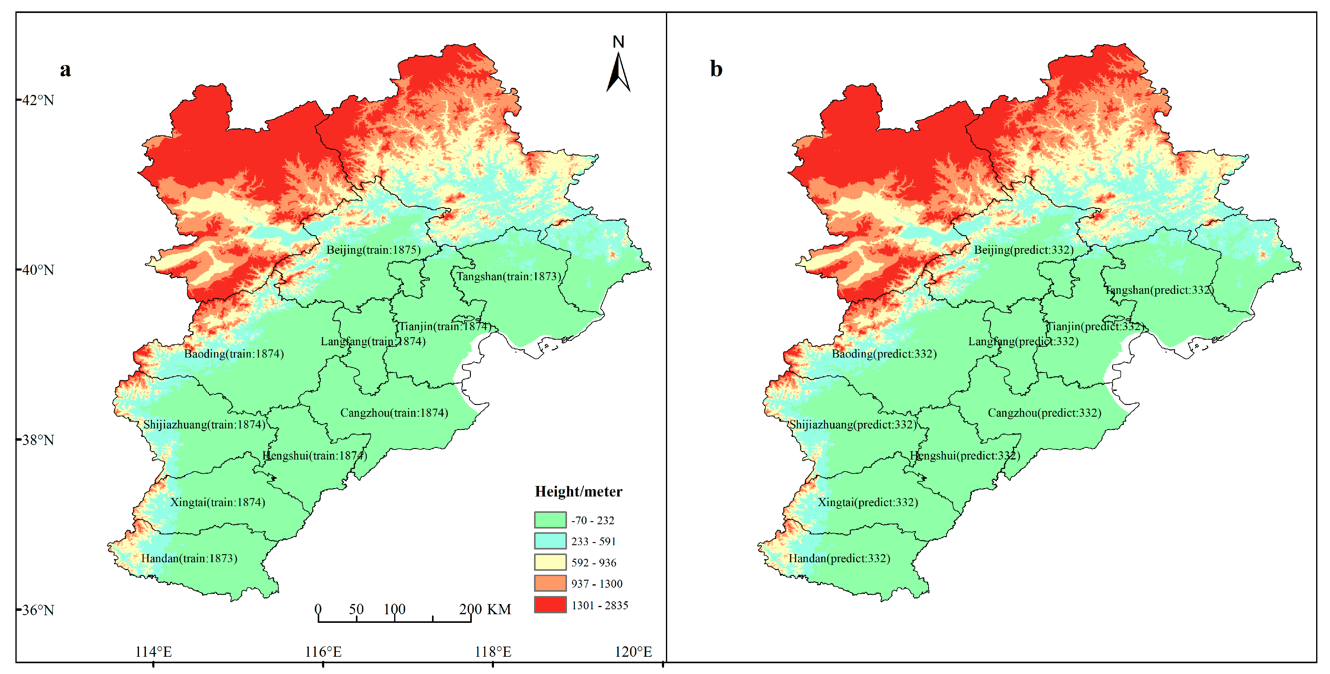
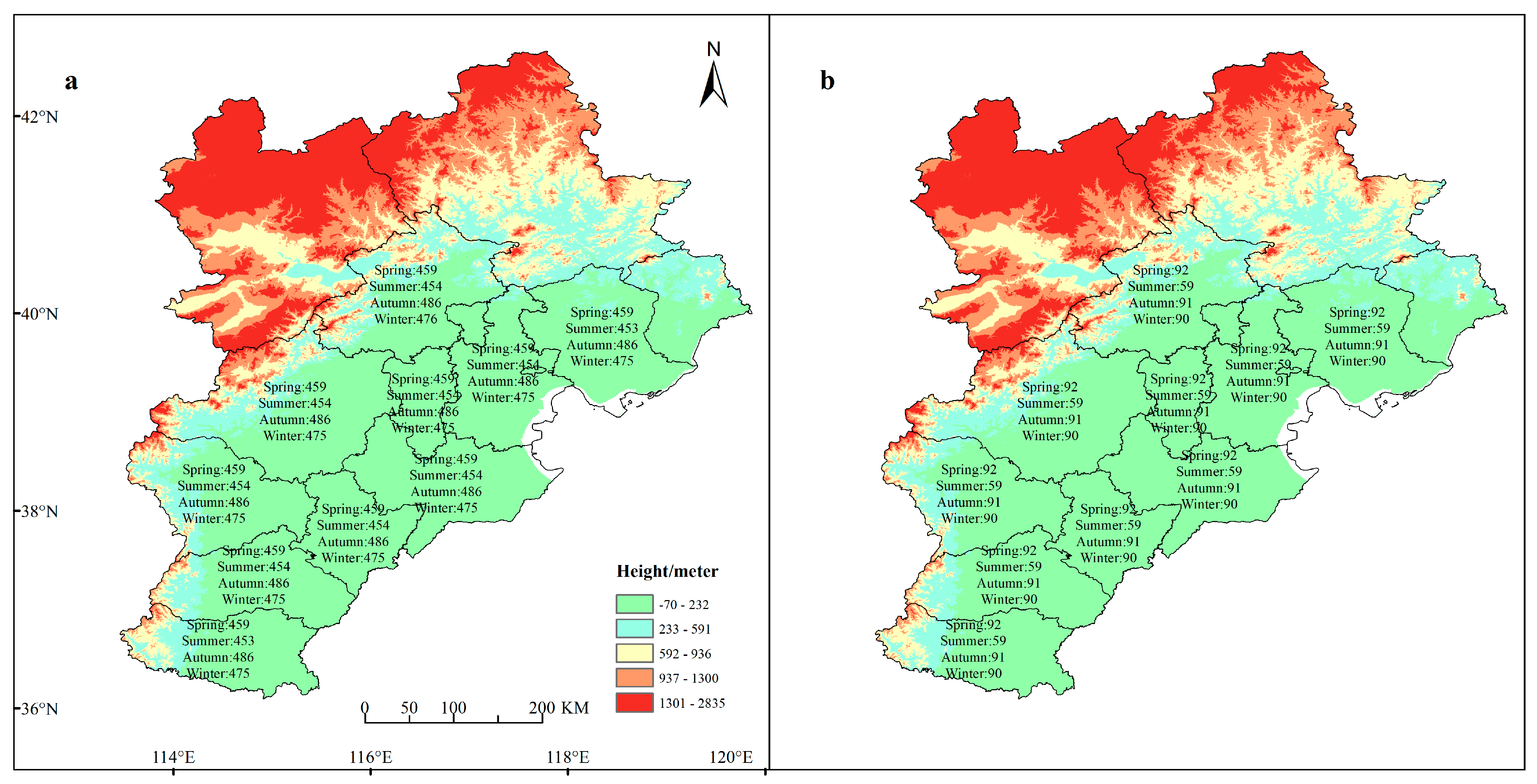
2.1. Data Description

Jing-Jin-Ji area is in the northeast of China (Figure 1), also known as Beijing-Tianjin-Hebei. China’s capital city Beijing occupies the core position of this region geographically and functionally. Therefore, Jing-Jin-Ji area is one of the three world-class urban clusters in China. Acting as the “capital economic circle”, this area also plays a crucial role in promoting the regional economic development of north China. Air pollution in this area is the most prominent environmental issue and has raised great concerns. Cities located in the atmospheric pollution transmission channel to Jing-Jin-Ji area are referred to as “2 + 26” channel cities (2 municipalities, 26 prefectures/cities) and for the first time are described in an officially launched government document. Ten urban monitoring stations of atmospheric transmission channels in the Jing-Jin-Ji region including Beijing, Tianjin, Baoding, Cangzhou, Handan, Hengshui, Langfang, Shijiazhuang, Tangshan, and Xingtai were selected in our research. The air quality data used in this study were downloaded from the China National Environmental Monitoring Centre (http://www.cnemc.cn (accessed on 1 July 2022)). The air quality indicators include air quality index (AQI), PM_2.5 concentration, PM₁₀ concentration, SO₂ concentration, NO₂ concentration, CO concentration, and O₃ concentration. Meteorological data were downloaded from China Weather (https://lishi.tianqi.com (accessed on 6 August 2022)), wherein meteorological types include the lowest temperature, the highest temperature, and wind speed. The dataset of overall 2206 days of monitoring data was used for model training and prediction.

We chose seven air quality indicators: PM₁₀, SO₂, NO₂, CO, O₃, AQI, AQI ranking, and three meteorological type indicators: lowest temperature, highest temperature, and wind speed. In addition, dummy variables were generated based on year, month, and season. To consider the historical data and enlarge the training dataset, the rolling training method was adopted by adding 1–5 previous days data into the input dataset. The selected feature dataset includes 29 variables (

Table 1. The feature selection of the dataset.

Selected Features
PM10	SO2	NO2	CO	O3	Lowest temperature	Highest temperature
Wind speed	Year	Month	Season	PM2.5_L1	PM2.5_L2	PM2.5_L3
PM2.5_L4	PM2.5_L5	AQI_L5	AQI ranking_L5	PM10_L5	SO2_L5	NO2_L5
CO_L5	O3_L5	Lowest temperature _L5	Highest temperature _L5	Wind speed _L5	Year_L5	Month_L5
Season_L5

Note: L1 is data of one day before and L5 is data of five days before.

). A total of 1874 days of monitoring sequence data from 28 October 2013 to 31 December 2018 were selected for model training and validation, and the remaining 332 days of monitoring sequence data from 1 January 2019 to 31 December 2019 were used as the testing dataset.

In the selected period, various statistical indicators of air quality and meteorological quality were calculated (

Table 2. Statistical summary of feature dataset.

	Unit	Mean	Variance	Minimum	25% Quantile	Median	75% Quantile	Maximum
AQI	____	116.41	5156.15	16	69	96	138	500
PM2.5	μg/m3	78.66	4374.42	0	36	59	98	796
PM10	μg/m3	134.76	8786.33	0	72	110	168	937
SO2	μg/m3	32.60	1220.53	0	11	21	40	437
NO2	μg/m3	48.32	559.85	0	31	44	61	235
CO	μg/m3	1.40	1.11	0	0.75	1.09	1.7	18.92
O3	μg/m3	57.98	1491.04	0	26	51	83	234
Lowest temperature	°C	8.72	117.92	−20	−2	9	19	29
Highest temperature	°C	19.05	123.20	−12	9	20	29	40
Wind speed	Force (Beaufort scale)	2.41	1.00	0	2	3	3	8

). For example, the minimum value of AQI was 16, the maximum value was 500, the variance was 5156.15, the mean was 116.41, the median was 96, the 25% quantile was 69, and the 75% quantile was 138. The minimum value of the PM_2.5 concentration was 0 μg/m³, the maximum was 796 μg/m³, the variance was 4374.42 μg/m³, the mean was 78.66 μg/m³, the median was 59 μg/m³, and the 25% quantile and the 75% quantile were 36 μg/m³ and 98 μg/m³, respectively.

The distribution characteristics of the data can be visually seen through the violin plots (Figure 2). The middle line is the median, and the two ends are the maximum and minimum values. According to the distribution pattern of each variable, the PM_2.5 concentration is skewed, and in the upper quartile, which is highly nonstationary and nonlinearity. Moreover, the distribution trend of AQI, PM₁₀, SO₂, NO₂, and O₃ is basically the same as that of PM_2.5, while the changing trend of CO, minimum temperature, highest temperature, wind speed, and PM_2.5 concentration is less consistent.

The distribution of training and test samples in the four seasons of each city site is shown in Figure 3 and Figure 4, where the number of samples drawn in each season is also relatively uniform. Therefore, the training results in the Beijing-Tianjin-Hebei region are spatially and temporally representative. The models obtained by training with RF, Ridge, LinearSVR, and ExtraTrees were used to predict the test set, divided into cities, and divided by seasons, and to conduct an empirical analysis of the prediction results.

The spatial distribution of training and test samples in the four seasons of each city site is shown in Figure 3 and Figure 4, where the number of samples drawn in each season is also relatively uniform. Therefore, the training results in the Beijing-Tianjin-Hebei region are spatially and temporally representative. The models obtained by training with RF, Ridge, LinearSVR, and ExtraTrees were used to predict the test set, divided into cities, and divided by seasons, and to conduct an empirical analysis of the prediction results.

To improve the generalization ability and accuracy of the prediction model, this paper adopts the idea of rolling prediction, using the historical monitoring data of the first five days to verify the PM_2.5 mass concentration of the next day, while successively rolling into models for training, verification, and learning. Considering that machine learning model training is more suitable for datasets with large sample sizes, in order to obtain enough training samples, the training data of the historical monitoring sequence of 10 cities in Beijing, Tianjin, and Hebei were combined with the determined feature variables into a new training matrix of 18,735 × 29. The corresponding target matrix is 18,735 × 1, accounting for 82.3% of the overall sample size, which is in line with the law of machine learning sample segmentation. Machine learning methods were respectively fed to the training dataset for K fold-over cross-training validation (K = 5).

The other 17.7% of the test dataset were 332 × 29 per city site, and the corresponding target matrix was 332 × 1. The distribution of the number of site samples in the training samples and test samples is shown in Figure 2, showing that the number of data samples extracted by each city site is relatively uniform.

2.2. Development of Predictive Models

2.2.1. Random Forest Model

First developed by Breiman, the random forest (RF) model is an integrated model based on the theory of decision trees [42]. It is a widely used machine learning method with good prediction accuracy. A random forest model draws multiple samples from the original sample by a resampling method and models each selected sample, and finally it obtains the final prediction results by averaging the predicted values of multiple decision trees. Random forests are multivariate nonlinear regression models, and the idea of “double random” makes random forests not easily fall into overfitting and creates diversity among the classifiers. Basic steps of the random forests are as follows:

(1)

Create the original dataset D;

$$D=\left\{\left(x_i,y_i\right),i=1,2,\cdots ,m\right\}{x}_i\in R^N,y_i\in R^N$$

(1)

In formula, y_i is the output and x_i is the input.

(2)

A subset is randomly selected from the dataset as the training dataset, where D_j is the training dataset of the jth iteration and j is the iteration number of the classifier (j = 1, 2 …, J). Each decision tree is constructed using a random subspace partition strategy, from which the optimal features are selected to split. After repeated training, Q decision trees are obtained and a random forest is formed.

(3)

The prediction result is the average value of each decision tree.

2.2.2. Ridge Regression Model

The coefficient estimation in the linear regression model depends on the independence of the model term, and the matrix (X^TX)⁻¹ becomes nearly singular if the term is relevant and the column of matrix X has an approximately linear correlation. Thus, the least squares estimation coefficients $\widehat{\beta }$ are highly sensitive to random errors in the response y, thus yielding large variances, and multicollinearity may occur, as shown in the following equation.

$$\widehat{\beta }=\left(X^{T}X\right)X^{T}y$$

(2)

Ridge regression (RR), also known as the Tikhonov regularization method, is a biased estimation regression method to solve the problem of data collinearity. Its essence is an improved least squares estimation method, which reduces the estimation variability by introducing the deviation into the coefficient estimation with the penalty term and makes the results more reliable. Ridge regression adopts Equation (3) to estimate the regression coefficient.

$$\widehat{\beta }=\left(X^{T}X+sH\right)X^{T}y$$

(3)

where s satisfies s > 0, it is called the ridge parameter or the bias parameter, and H is the unit matrix.

2.2.3. Support Vector Machine Model

Support vector machine (SVM) is a maximum-interval classification algorithm proposed by Vapnik, which enables the linear separation of the samples by mapping the samples to a higher-dimensional feature space and introduces the kernel function to realize the nonlinear mapping [43]. Support vector regression (SVR) which uses a deep learning mechanism is developed and optimized based on SVM. Compared with neural networks, support vector regression can overcome the problems of overfitting, underfitting, and local optimization by using mathematical methods and optimization techniques. Given the Dataset D:

$$D=\left\{\left(x_i,y_i\right),i=1,2,\cdots ,m\right\}{x}_i\in R^N,y_i\in R^N$$

(4)

The hyperplane model for constructing the high-dimensional space division is as follows:

$$f\left(x\right)=w^T\varphi \left(x\right)+\vartheta$$

(5)

Among them, f(x) is the prediction value, φ(x) is the nonlinear mapping function, w is the weight coefficient, ϑ is the intercept term, and ε is the error interval bandwidth. Only when the training sample falls in the interval band are prediction results considered correct. Therefore, by introducing the relaxation variable ${\xi }_i$, ${\widehat{\xi }}_i$and the penalty function E, the optimized objective function is obtained:

$$\underset{w,\vartheta ,{\xi }_i,{\widehat{\xi }}_i}{Min}\frac{1}{2}{\Vert w\Vert }^2+E{{\displaystyle \sum }}_{i=1}^m\left({\xi }_i+{\widehat{\xi }}_i\right)$$

(6)

$$\mathrm{s}.\mathrm{t} \left\{\begin{array}{c}f\left(x_i\right)-y_i\le \epsilon +{\xi }_i\hfill \\ y_i-f\left(x_i\right)\le \epsilon +{\widehat{\xi }}_i\hfill \\ {\xi }_i\ge 0,{\widehat{\xi }}_i\ge 0,i=1,2,\cdots ,m\hfill \end{array}\right.$$

The “dual problem” of support vector regression can be formed by adopting a Lagrangian multiplier. The optimal Lagrangian multiplier can be solved by the sequence minimum optimization (SMO) algorithm, and the final solution is obtained according to the KKT (Karush-Kuhn-Tucker, KKT) condition:

$$f\left(x\right)={{\displaystyle \sum }}_{i=1}^m\left({\widehat{\lambda }}_i-{\lambda }_i\right)K\left(x_i^T{x}_i\right)+\vartheta$$

(7)

where, ${\lambda }_i$ and ${\widehat{\lambda }}_i$ are Lagrange multipliers and $K\left(x_i^T{x}_i\right)$ is kernel functions.

2.2.4. Extremely Randomized Trees Model

The extremely randomized trees (ExtraTrees), which is a variant of the random forest and includes many decision trees, is an integrated learning algorithm [44]. The prominent feature of this algorithm is the selection of the splitting features. A certain value of a certain feature is randomly selected as the split point of the feature, and the result is jointly determined by the output results of the many decision trees contained in it. Therefore, the extremely randomized trees algorithm has strong generalization ability and a certain level of resistance to noise perturbations.

2.3. Evaluation Metrics

To compare the predictive performance of four models, the prediction effect of each machine learning algorithm was evaluated by using the mean absolute error (MAE), root mean square error (RMSE), index of agreement (IA), and determination coefficient (R²).

The average absolute error is the average of the absolute value of the deviation between all individual observations and the arithmetic mean. This index can avoid the problem of the errors canceling each other and can reflect the scale of the actual prediction error more accurately.

$$MAE\left(y,\widehat{y}\right)=\frac{1}{m}{{\displaystyle \sum }}_{i=1}^m\left|y_i-{\widehat{y}}_i\right|$$

(8)

The RMSE is the square root of the mean of the square of all of the errors.

$$RMSE\left(y,\widehat{y}\right)=\sqrt{\frac{1}{m}{{\displaystyle \sum }}_{i=1}^m{\left(y_i-{\widehat{y}}_i\right)}^2}$$

(9)

The closer the index of agreement (IA) is to 1, the higher the changing trend and consistency degree of the predicted value and the measured value.

$$IA=1-\frac{{{\displaystyle \sum }}_{i=1}^m{\left(y_i-{\widehat{y}}_i\right)}^2}{{{\displaystyle \sum }}_{i=1}^m{\left(\left|{\widehat{y}}_i-\stackrel{-}{y}\right|+\left|y_i-\stackrel{-}{y}\right|\right)}^2}$$

(10)

The coefficient of determination (R²) indicates the fitting level of the predictive model.

$$R^2\left(y,\widehat{y}\right)=1-\frac{SSE}{SST}=1-\frac{{{\displaystyle \sum }}_{i=1}^m{\left(y_i-{\widehat{y}}_i\right)}^2}{{{\displaystyle \sum }}_{i=1}^m{\left(y_i-{\stackrel{-}{y}}_i\right)}^2}$$

(11)

3. Results

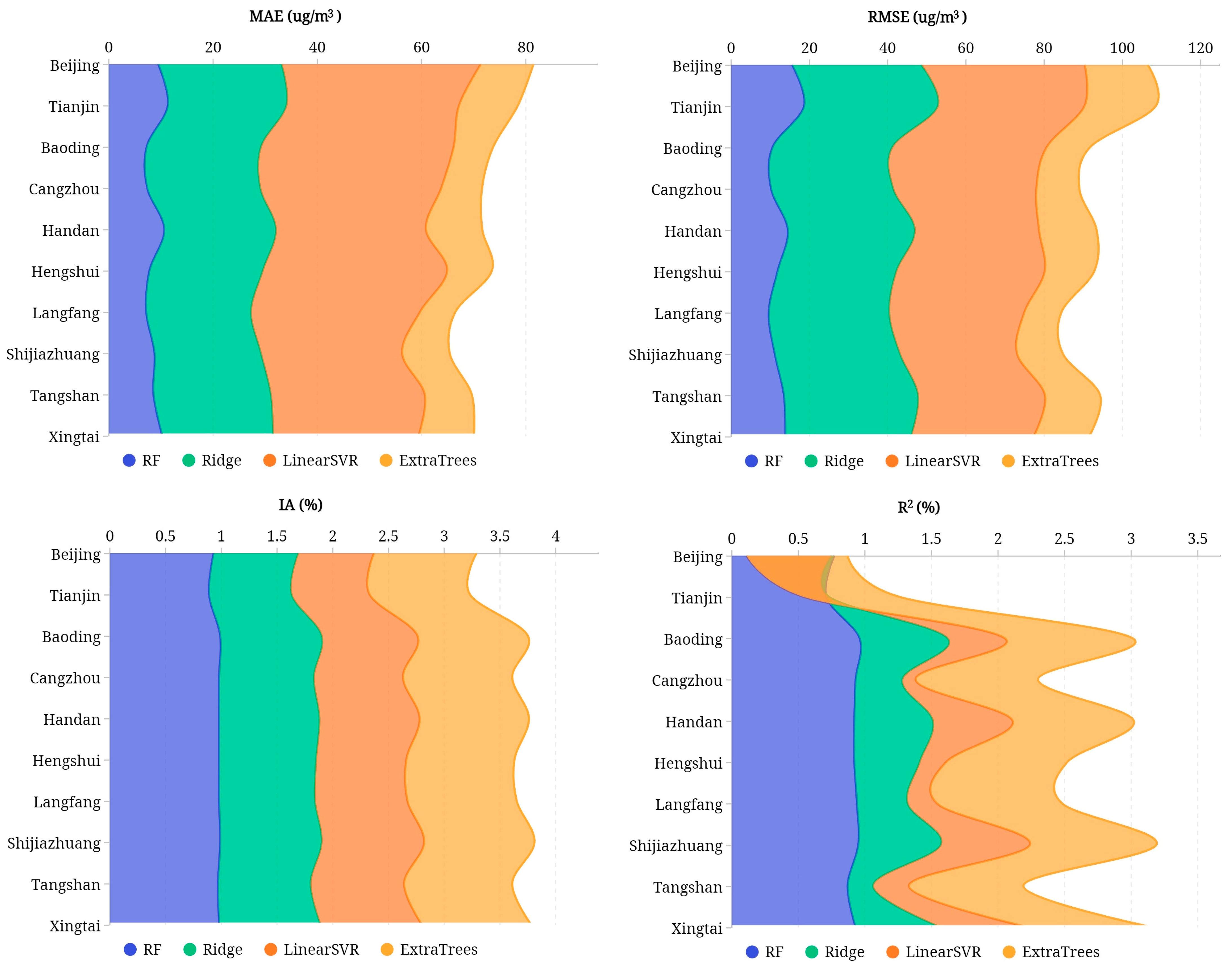
3.1. Prediction Comparison Based on City Level

The experiment was first conducted on 10 monitoring sites, wherein we compared the PM_2.5 prediction results generated by machine learning models RF, Ridge, LinearSVR, and ExtraTrees for each city by calculating the MAE, RMSE, IA, and R² (

Table 3. Prediction results for each city.

City		RF	Ridge	LinearSVR	ExtraTrees
Beijing	MAE	9.47	23.64	38.26	10.08
	RMSE	15.56	32.98	41.85	16.09
	IA	0.93	0.76	0.68	0.92
	R2	0.77	−0.02	−0.64	0.76
Tianjin	MAE	11.33	22.72	33.13	11.30
	RMSE	18.64	34.17	37.50	18.23
	IA	0.89	0.74	0.70	0.90
	R2	0.71	0.02	−0.19	0.72
Baoding	MAE	7.26	21.92	36.98	7.59
	RMSE	10.57	30.57	39.48	11.07
	IA	0.99	0.91	0.86	0.99
	R2	0.96	0.66	0.43	0.96
Cangzhou	MAE	7.36	21.69	34.73	7.81
	RMSE	10.21	31.22	36.60	10.99
	IA	0.98	0.85	0.80	0.98
	R2	0.93	0.35	0.10	0.92
Handan	MAE	10.65	21.40	28.79	10.79
	RMSE	14.51	32.44	31.75	14.72
	IA	0.98	0.90	0.90	0.98
	R2	0.92	0.59	0.60	0.91
Hengshui	MAE	7.80	21.72	35.40	8.58
	RMSE	11.87	30.33	37.96	12.66
	IA	0.98	0.87	0.81	0.97
	R2	0.92	0.49	0.20	0.91
Langfang	MAE	7.17	20.10	32.44	6.77
	RMSE	9.62	30.79	34.52	9.46
	IA	0.98	0.86	0.83	0.98
	R2	0.94	0.38	0.22	0.94
Shijiazhuang	MAE	8.77	20.40	27.09	9.12
	RMSE	11.15	31.99	29.97	11.70
	IA	0.99	0.91	0.92	0.99
	R2	0.95	0.62	0.67	0.95
Tangshan	MAE	8.57	22.50	29.54	9.01
	RMSE	13.49	34.28	32.46	14.10
	IA	0.97	0.83	0.84	0.97
	R2	0.87	0.19	0.27	0.86
Xingtai	MAE	10.26	21.23	27.94	10.58
	RMSE	13.85	32.08	31.42	14.16
	IA	0.98	0.91	0.91	0.98
	R2	0.93	0.64	0.66	0.93

). The MAE results show that two major cities, i.e., Beijing and Tianjin, had relatively high values and MAEs of the remaining eight cities were relatively low. As can be seen in Figure 5, the MAEs of RF and ExtraTrees were both concentrated around 10 μg/m³, and Ridge model’s MAE was concentrated at 21 μg/m³, and the MAE of LinearSVR model was scattered in the interval of 27.09~38.26 μg/m³. The MAE of RF and ExtraTrees were significantly better than that of Ridge model, and LinearSVR model had the worst result.

The comparison of RMSE shows that the PM_2.5 concentration and observed values predicted by the RF model was 9.62~18.64 μg/m³, 9.46~18.23 μg/m³ for the ExtraTrees model, Ridge model was 30.32~34.28 μg/m³, and 29.97~41.85 μg/m³ for the LinearSVR model. The RMSE of the RF and ExtraTrees models were the smallest. The PM_2.5 concentration in Beijing, Baoding, Cangzhou, Handan, Hengshui, Shijiazhuang, Tangshan, and Xingtai urban stations predicted by the RF model were slightly less than ExtraTrees’s prediction result, while the remaining two urban stations were slightly greater than ExtraTrees.

IA of Ridge model’s predicted PM_2.5 and observants ranged from 0.74~0.91, while for the LinearSVR model this was 0.68~0.92. Among all sampled cities, only Beijing and Tianjin’s IA values were smaller than 0.8. The IA values of RF model and ExtraTrees model were 0.89~0.99 and 0.90~0.99, respectively. Lower IA values were attained in Beijing and Tianjin monitoring sites, which is consistent with the results of Ridge and LinearSVR. The IA of PM_2.5 concentration in Beijing, Baoding, Cangzhou, Handan, Hengshui, Shijiazhuang, Tangshan, and Xingtai monitoring sites were slightly higher than ExtraTrees, while the other two urban stations were slightly lower than ExtraTrees, which is consistent with the results of RMSE. Overall, the RF and ExtraTrees were significantly better than the Ridge and LinearSVR models, while RF was slightly better than ExtraTrees.

Table 4. Distribution range of deviation between predictions and observed values in observing cites.

City	RF		Ridge		LinearSVR		ExtraTrees
	90%	75%	90%	75%	90%	75%	90%	75%
Beijing	−20–32	−14–9	−29–159	−26–60	−55–61	−52–−20	−21–36	−17–7
Tianjin	−22–44	−17–10	−25–173	−18–65	−54–70	−45–−13	−23–44	−16–9
Baoding	−13–40	−10–9	−25–145	−20–58	−52–47	−48–−21	−13–33	−11–10
Cangzhou	−14–39	−10–11	−21–176	−18–63	−48–78	−45–−19	−15–41	−11–10
Handan	−7–47	−5–21	−18–107	−16–67	−46–42	−41–−8	−11–52	−7–20
Hengshui	−16–34	−12–9	−24–91	−20–60	−52–12	−48–−19	−19–32	−13–8
Langfang	−7–34	−6–14	−19–166	−16–65	−46–63	−43–−17	−9–38	−6–11
Shijiazhuang	−9–39	−6–16	−16–105	−14–69	−44–47	−39–−9	−10–35	−6–16
Tangshang	−7–88	−5–17	−20–187	−17–65	−45–87	−43–−11	−8–93	−4–17
Xingtai	−14–60	−9–16	−19–110	−15–65	−45–47	−41–−9	−16–56	−11–15

shows the distribution of prediction deviation for each city. The prediction deviation of the RF model was distributed in the range −22~88 μg/m³, wherein 75% of the deviation was concentrated within −17~21 μg/m³. The Ridge model predictions deviation was distributed from −29 to 187 μg/m³, of which 75% was concentrated within −26~69 μg/m³. LinearSVR prediction deviation was distributed from −55 to 87 μg/m³, of which 75% was concentrated within −52~−8 μg/m³. ExtraTrees prediction deviation was distributed from −23 to 93 μg/m³, of which 75% was concentrated within −17~20 μg/m³. The deviation values of LinearSVR were significantly biased towards negative values, Ridge’s maximum probability distribution had a wide range, the deviation of the RF and ExtraTrees were centered around 0, and the maximum probability distribution was narrower, more concentrated, and more effective.

In Figure 6, the prediction deviation curve of PM_2.5 concentration is consistent with the above results.

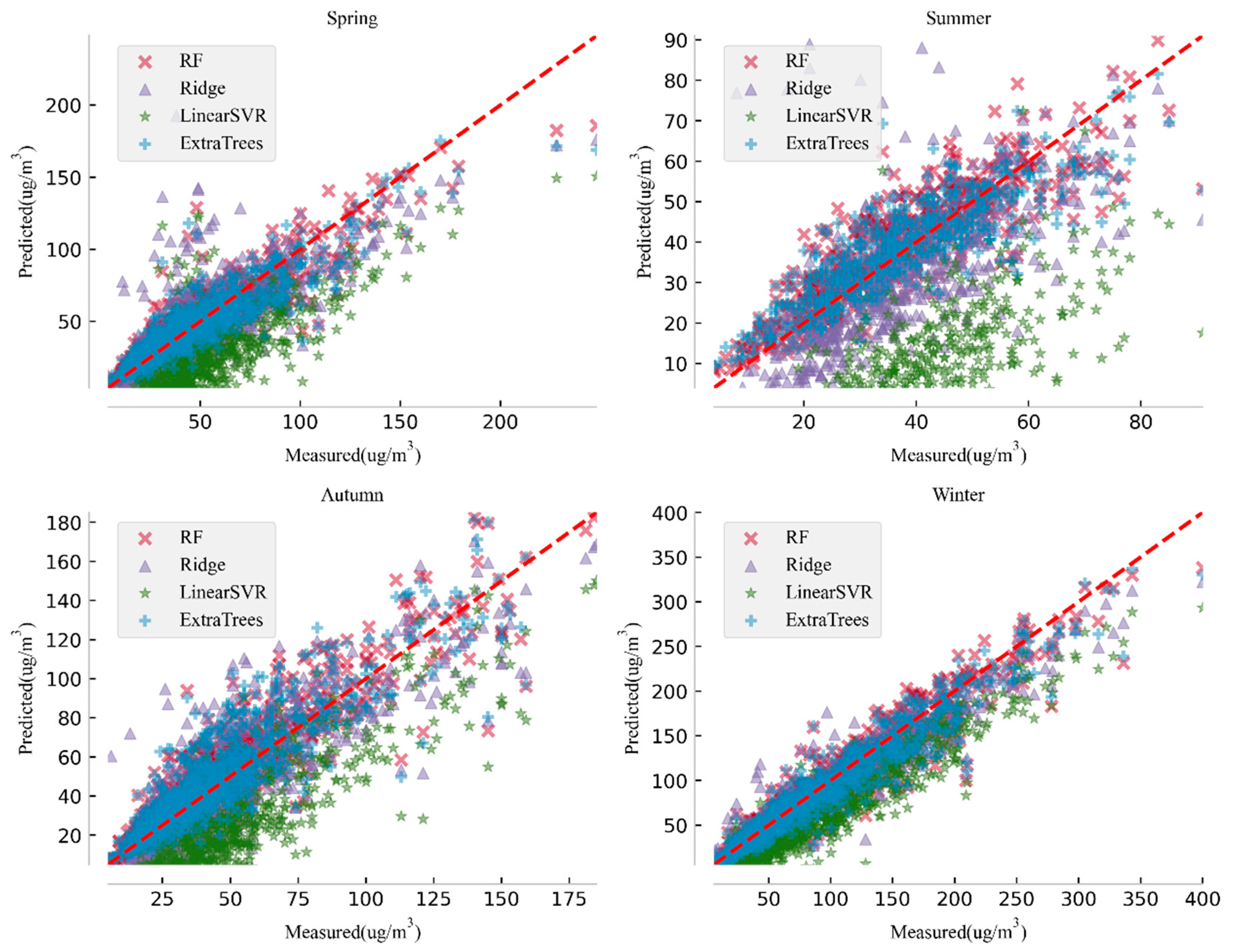
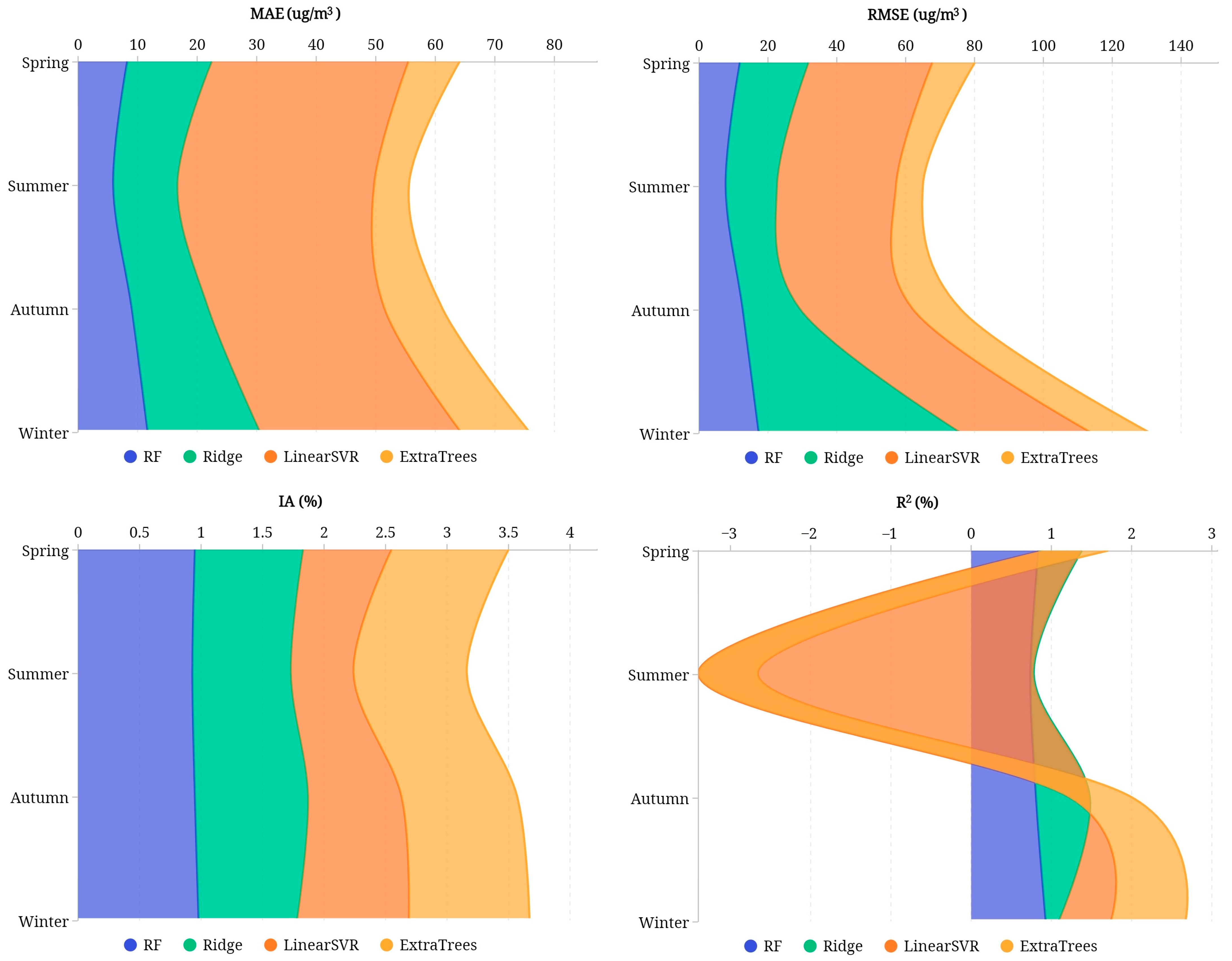
3.2. Prediction Comparison Based on Seasons

Figure 7 shows the prediction deviation for PM_2.5 concentration of four seasons in 2019. Combining the IA and the MAE of the different seasons in

Table 5. Evaluation on the prediction results of four models for each season.

		RF	Ridge	LinearSVR	ExtraTrees
Spring	MAE	8.26	14.21	33.02	8.61
	RMSE	11.87	19.94	35.98	12.31
	IA	0.95	0.88	0.72	0.95
	R2	0.84	0.54	−0.49	0.82
Summer	MAE	5.91	10.77	33.04	5.84
	RMSE	7.75	14.89	34.55	7.78
	IA	0.93	0.80	0.51	0.92
	R2	0.74	0.04	−4.18	0.74
Autumn	MAE	9.02	12.86	29.58	9.73
	RMSE	12.71	16.72	32.78	13.84
	IA	0.95	0.92	0.76	0.94
	R2	0.81	0.67	−0.25	0.78
Winter	MAE	11.68	18.89	33.74	11.50
	RMSE	17.35	58.81	38.01	16.94
	IA	0.98	0.80	0.91	0.98
	R2	0.93	0.16	0.65	0.93

, in the Jing-Jin-Ji region the overall effect of RF, Ridge, LinearSVR, and ExtraTrees models on the seasonal PM_2.5 concentration prediction shows that four models all have the best predicative results in winter and the worst in summer. It is assumed that air particulate pollution in the Jing-Jin-Ji region is the worst in winter, and the PM_2.5 concentrations were much higher than in the other three seasons, while particulate pollution is less prominent in summer. The RF model prediction’s IA ranges from 0.93 to 0.98, with an MAE of 5.91 to 11.68 μg/m³, converging with the ExtraTrees predicative performance, and outperformed Ridge and LinearSVR overall.

In summer, Ridge and LinearSVR models have IA of 0.8 and 0.51, respectively, while in winter, Ridge and LinearSVR models have IA of 0.8 and 0.91, which shows that Ridge was better than LinearSVR in summer and worse than LinearSVR in winter (Figure 8).

3.3. Overall Evaluation

According to

Table 6. Model construction time and occupied memory size.

Model	Occupied Memory Size (KB)	Model Construction Time (S)
RF	136,192	63.96
Ridge	3.79	2.27
Linear SVR	3.81	8.07
Extra Trees	227,328	28.22

, the RF model had the longest construction time, followed by ExtraTrees, and the shortest Ridge construction time was 2.27 s. In terms of model memory usage, the ExtraTrees occupies the largest memory, the model size was 222 MB, followed by the RF model, the memory usage size was 133 MB, the smallest model was Ridge, and the memory size was only 3.79 KB.

4. Discussion

This study agrees with the findings of the research done by Wang and colleagues [45] who selected six monitoring sites located in Guangdong province and who proved that differences exist in PM_2.5 concentration predications for each monitoring site because of the spatial heterogeneity. However, such existing similar research lacks the discussion of seasonal comparisons and the systematic classification and research on influencing factors of air pollution prediction are still missing. Our research is designed to fill this gap. Urban is a complex gigantic system and it is composed of many sub-systems, notably, society, economy, and environment. On the level of sub-system, basic units can function properly with their own principles; however, emergence occurs as a result of the interactions of basic units from different sub-systems. For instance, environmental issues are the consequences of human activities in the complex urban system and their magnitude is strongly associated with multiple interconnected factors. Nevertheless, they are not simply the linear accumulation of individual factor effects, since chaotic characteristics have been observed in time series air pollution data [46,47]. Further, these factors can be roughly categorized into four types: urban development properties (urbanization rate, city industrial structure, GDP, etc.), energy consumption status (energy consumption structure, energy utility efficiency, etc.), infrastructure construction (transportation infrastructure, green infrastructure, etc.), and environmental management policies (pollution management and control policies, environmental financial policies, etc.).

Urban development properties are the core character of urban systems and represent the basic status of urban growth, while meanwhile offering a set of scientific measurements for urban performance. Further, urban development properties are the dominant factors in determining the urban development mode. For instance, in the study area the capital cities such as Beijing and Tianjin with higher urbanization rates, are such that their tertiary industries tend to occupy larger portions in the overall industrial structure compared to other cities. As a result, those cities are characterized by green energy consumption structure and higher energy utility efficiency. In contrast, some other cities such as Tangshan and Handan which excessively rely on heavy industries are facing more serious air pollution pressure. Especially when some of those cities were designated as the outflow area for the industrial transfer of particularly iron and steel production and construction material production industries, the air pollution issues become aggravated [48].

Given the current energy structure in China, energy consumption intensity relates very closely with industrial structure. Consequently, cities in the study area exhibit various characteristics in energy consumption due to different industrial structure. The unreasonable energy consumption structure has been a long-lasting and prominent problem. In Hebei province, coal consumption occupies over 70% of the total energy consumption, higher than the national level of 56.8% in 2021. In 2017, the total coal consumption of Tangshan was 15.3 times of this value in Beijing [49].

Urban infrastructure constructs the physical foundation of urban human habitat, offers the platform and channel for material and energy, and also generates pollutants transferring and exchanging [50,51]. Along with processes of urbanization, the elements cycle has been deeply interfered with by human activities. Urban functional zone layout and transportation infrastructure are the hardware for the reconstructed living habitat. Proper design can help alleviate the so-called urban diseases including severe air pollution. For example, to balance the land use of industrial use and green space, efforts include equal development of residential and industrial zones to shorten the commute distance in the aim of reducing transportation air pollution [52] and smart transportation infrastructure design.

Unlike the first three factors, environmental management policies are designed for environmental protection purposes; therefore, it plays a crucial role in air pollutant concentration status. Owing to China’s efficient administrative system, normally the environmental regulations on a certain industry or a certain enterprise are very effectively accurate, which will inevitably cause sudden changes to air pollutants concentration, thus leading to noise data for the model prediction. Therefore, more attention should be paid when processing data with noise.

In addition to the abovementioned four urban related influencing factors, it is also very important to factor the seasonal elements into interpreting the different performances of each model for each city. While the local government is putting on stricter air pollution control regulations, the air pollution condition has been improved substantially, but new characteristics were discovered. For example, the air pollution becomes worse in winter time, while in summer time the pollution status will be substantially alleviated. This is partially because in the rural area in north China coal burning is still the primary method for heating.

However, there are still some restrictions and limitations of this research, for it still lacks consideration of various influencing factors, such as GDP, energy structure, etc. Furthermore, more advanced artificial neural network models can be discussed and adopted to gain higher prediction accuracy. For instance, Convolution Neural Network (CNN) can be adopted to further enhance the prediction accuracy and increase the applicability and decrease the dimension of features and the training time required to train the model, thus substantially enhancing the prediction capacity.

5. Conclusions

Research on model training and comparison is of great importance in guiding air pollution control and management policymaking processes. Our study chose ten atmospheric pollution transmission channel cities located in the Jing-Jin-Ji area for the study area, whereby air quality features, meteorological features, time features, and historical features data from the ten monitoring sites were collected to train the models. Fed with the multi-sourced data, four selected models—random forest model, ridge regression model, support vector machine model, extremely randomized trees model—were trained and produced predicative results. Comparison analysis was then conducted on city level and season level and further environmental management advice was given.

The comparison on city level shows that RF and ExtraTrees are significantly better than the Ridge and LinearSVR models, while RF is slightly better than ExtraTrees. The RMSE of the RF and ExtraTrees models are the smallest. Among all sampled cities, only Beijing and Tianjin’s IA values are smaller than 0.8. The comparison on season level shows that the RF model prediction’s IA ranges from 0.93 to 0.98, with an MAE of 5.91 to 11.68 μg/m³, converging with the ExtraTrees predicative performance, and outperforming Ridge and LinearSVR overall.

References

1. Lewis, S.L.; Maslin, M.A. Defining the anthropocene. Nature 2015, 519, 171–180. [Google Scholar] [CrossRef]
2. Steffen, W.; Grinevald, J.; Crutzen, P.; McNeill, J. The Anthropocene: Conceptual and historical perspectives. Philos. Trans. R. Soc. A Math. Phys. Eng. Sci. 2011, 369, 842–867. [Google Scholar] [CrossRef]
3. Lelieveld, J. Clean air in the Anthropocene. Faraday Discuss. 2017, 200, 693–703. [Google Scholar] [CrossRef]
4. Xing, Y.; Xu, Y.; Shi, M.; Lian, Y. The impact of PM2.5 on the human respiratory system. J. Thorac. Dis. 2016, 8, E69. [Google Scholar]
5. Apte, J.S.; Brauer, M.; Cohen, A.J.; Ezzati, M.; Pope, C.A., III. Ambient PM2.5 reduces global and regional life expectancy. Environ. Sci. Technol. Lett. 2018, 5, 546–551. [Google Scholar] [CrossRef]
6. Al-Hemoud, A.; Gasana, J.; Al-Dabbous, A.; Alajeel, A.; Al-Shatti, A.; Behbehani, W.; Malak, M. Exposure levels of air pollution (PM2.5) and associated health risk in Kuwait. Environ. Res. 2019, 179, 108730. [Google Scholar] [CrossRef] [PubMed]
7. Feng, S.; Gao, D.; Liao, F.; Zhou, F.; Wang, X. The health effects of ambient PM2.5 and potential mechanisms. Ecotoxicol. Environ. Saf. 2016, 128, 67–74. [Google Scholar] [CrossRef] [PubMed]
8. McDuffie, E.E.; Martin, R.V.; Spadaro, J.V.; Burnett, R.; Smith, S.J.; O’Rourke, P.; Hammer, M.S.; van Donkelaar, A.; Bindle, L.; Shah, V. Source sector and fuel contributions to ambient PM2.5 and attributable mortality across multiple spatial scales. Nat. Commun. 2021, 12, 3594. [Google Scholar] [CrossRef] [PubMed]
9. Huang, C.; Hu, J.; Xue, T.; Xu, H.; Wang, M. High-resolution spatiotemporal modeling for ambient PM2.5 exposure assessment in China from 2013 to 2019. Environ. Sci. Technol. 2021, 55, 2152–2162. [Google Scholar] [CrossRef]
10. Chakrabarty, R.K.; Beeler, P.; Liu, P.; Goswami, S.; Harvey, R.D.; Pervez, S.; van Donkelaar, A.; Martin, R.V. Ambient PM2.5 exposure and rapid spread of COVID-19 in the United States. Sci. Total Environ. 2021, 760, 143391. [Google Scholar] [CrossRef]
11. Cao, J.; Chow, J.C.; Lee, F.S.; Watson, J.G. Evolution of PM2.5 measurements and standards in the US and future perspectives for China. Aerosol Air Qual. Res. 2013, 13, 1197–1211. [Google Scholar] [CrossRef]
12. Chow, J.; Watson, J.; Cao, J. Highlights from Leapfrogging Opportunities for Air Quality Improvement. EM 2010, 16, 38–43. [Google Scholar]
13. Shin, S.E.; Jung, C.H.; Kim, Y. Analysis of the measurement difference for the PM10 concentrations between Beta-ray absorption and gravimetric methods at Gosan. Aerosol Air Qual. Res. 2011, 11, 846–853. [Google Scholar] [CrossRef]
14. Takahashi, K.; Minoura, H.; Sakamoto, K. Examination of discrepancies between beta-attenuation and gravimetric methods for the monitoring of particulate matter. Atmos. Environ. 2008, 42, 5232–5240. [Google Scholar] [CrossRef]
15. Tasić, V.; Jovašević-Stojanović, M.; Vardoulakis, S.; Milošević, N.; Kovačević, R.; Petrović, J. Comparative assessment of a real-time particle monitor against the reference gravimetric method for PM10 and PM2.5 in indoor air. Atmos. Environ. 2012, 54, 358–364. [Google Scholar] [CrossRef]
16. Karagulian, F.; Belis, C.A.; Dora, C.F.C.; Prüss-Ustün, A.M.; Bonjour, S.; Adair-Rohani, H.; Amann, M. Contributions to cities’ ambient particulate matter (PM): A systematic review of local source contributions at global level. Atmos. Environ. 2015, 120, 475–483. [Google Scholar] [CrossRef]
17. Singh, N.; Murari, V.; Kumar, M.; Barman, S.C.; Banerjee, T. Fine particulates over South Asia: Review and meta-analysis of PM2.5 source apportionment through receptor model. Environ. Pollut. 2017, 223, 121–136. [Google Scholar] [CrossRef]
18. Saraga, D.E.; Tolis, E.I.; Maggos, T.; Vasilakos, C.; Bartzis, J.G. PM2.5 source apportionment for the port city of Thessaloniki, Greece. Sci. Total Environ. 2019, 650, 2337–2354. [Google Scholar] [CrossRef]
19. Zheng, M.; Salmon, L.G.; Schauer, J.J.; Zeng, L.; Kiang, C.S.; Zhang, Y.; Cass, G.R. Seasonal trends in PM2.5 source contributions in Beijing, China. Atmos. Environ. 2005, 39, 3967–3976. [Google Scholar] [CrossRef]
20. Zhang, X.; Ji, G.; Peng, X.; Kong, L.; Zhao, X.; Ying, R.; Yin, W.; Xu, T.; Cheng, J.; Wang, L. Characteristics of the chemical composition and source apportionment of PM2.5 for a one-year period in Wuhan, China. J. Atmos. Chem. 2022, 79, 101–115. [Google Scholar] [CrossRef]
21. Zhang, Y.; Cai, J.; Wang, S.; He, K.; Zheng, M. Review of receptor-based source apportionment research of fine particulate matter and its challenges in China. Sci. Total Environ. 2017, 586, 917–929. [Google Scholar] [CrossRef]
22. Liu, P.; Zhang, C.; Xue, C.; Mu, Y.; Liu, J.; Zhang, Y.; Tian, D.; Ye, C.; Zhang, H.; Guan, J. The contribution of residential coal combustion to atmospheric PM2.5 in northern China during winter. Atmos. Chem. Phys. 2017, 17, 11503–11520. [Google Scholar] [CrossRef]
23. Askariyeh, M.H.; Khreis, H.; Vallamsundar, S. Chapter 5—Air pollution monitoring and modeling. In Traffic-Related Air Pollution; Khreis, H., Nieuwenhuijsen, M., Zietsman, J., Ramani, T., Eds.; Elsevier: Amsterdam, The Netherlands, 2020; pp. 111–135. [Google Scholar]
24. Hu, J.; Ostro, B.; Zhang, H.; Ying, Q.; Kleeman, M.J. Using chemical transport model predictions to improve exposure assessment of PM2.5 constituents. Environ. Sci. Technol. Lett. 2019, 6, 456–461. [Google Scholar]
25. Polat, E.; Gunay, S. The comparison of partial least squares regression, principal component regression and ridge regression with multiple linear regression for predicting pm10 concentration level based on meteorological parameters. J. Data Sci. 2015, 13, 663–692. [Google Scholar] [CrossRef]
26. Singh, K.P.; Gupta, S.; Kumar, A.; Shukla, S.P. Linear and nonlinear modeling approaches for urban air quality prediction. Sci. Total Environ. 2012, 426, 244–255. [Google Scholar] [CrossRef] [PubMed]
27. Sampson, P.D.; Richards, M.; Szpiro, A.A.; Bergen, S.; Sheppard, L.; Larson, T.V.; Kaufman, J.D. A regionalized national universal kriging model using Partial Least Squares regression for estimating annual PM2.5 concentrations in epidemiology. Atmos. Environ. 2013, 75, 383–392. [Google Scholar] [CrossRef] [PubMed]
28. Faganeli Pucer, J.; Pirš, G.; Štrumbelj, E. A Bayesian approach to forecasting daily air-pollutant levels. Knowl. Inf. Syst. 2018, 57, 635–654. [Google Scholar] [CrossRef]
29. Liu, Y.; Guo, H.; Mao, G.; Yang, P. A Bayesian hierarchical model for urban air quality prediction under uncertainty. Atmos. Environ. 2008, 42, 8464–8469. [Google Scholar] [CrossRef]
30. Sun, W.; Zhang, H.; Palazoglu, A.; Singh, A.; Zhang, W.; Liu, S. Prediction of 24-h-average PM2.5 concentrations using a hidden Markov model with different emission distributions in Northern California. Sci. Total Environ. 2013, 443, 93–103. [Google Scholar] [CrossRef]
31. Ni, X.Y.; Huang, H.; Du, W. Relevance analysis and short-term prediction of PM2.5 concentrations in Beijing based on multi-source data. Atmos. Environ. 2017, 150, 146–161. [Google Scholar] [CrossRef]
32. Zhang, Z.; Jiang, Z.; Meng, X.; Cheng, S.; Sun, W. Research on prediction method of api based on the enhanced moving average method. In Proceedings of the 2012 International Conference on Systems and Informatics (ICSAI2012), Yantai, China, 19–20 May 2012. [Google Scholar]
33. Kumar, U.; Jain, V.K. ARIMA forecasting of ambient air pollutants (O3, NO, NO2 and CO). Stoch. Environ. Res. Risk Assess. 2010, 24, 751–760. [Google Scholar] [CrossRef]
34. Abhilash, M.; Thakur, A.; Gupta, D.; Sreevidya, B. Time series analysis of air pollution in Bengaluru using ARIMA model. In Ambient Communications and Computer Systems; Springer: Berlin/Heidelberg, Germany, 2018; pp. 413–426. [Google Scholar]
35. Bhatti, U.A.; Yan, Y.; Zhou, M.; Ali, S.; Hussain, A.; Qingsong, H.; Yu, Z.; Yuan, L. Time series analysis and forecasting of air pollution particulate matter (PM2.5): An SARIMA and factor analysis approach. IEEE Access 2021, 9, 41019–41031. [Google Scholar] [CrossRef]
36. Niu, M.; Wang, Y.; Sun, S.; Li, Y. A novel hybrid decomposition-and-ensemble model based on CEEMD and GWO for short-term PM2.5 concentration forecasting. Atmos. Environ. 2016, 134, 168–180. [Google Scholar] [CrossRef]
37. Liao, K.; Huang, X.; Dang, H.; Ren, Y.; Zuo, S.; Duan, C. Statistical approaches for forecasting primary air pollutants: A review. Atmosphere 2021, 12, 686. [Google Scholar] [CrossRef]
38. Masood, A.; Ahmad, K. A model for particulate matter (PM2.5) prediction for Delhi based on machine learning approaches. Procedia Comput. Sci. 2020, 167, 2101–2110. [Google Scholar] [CrossRef]
39. Ordieres, J.B.; Vergara, E.P.; Capuz, R.S.; Salazar, R.E. Neural network prediction model for fine particulate matter (PM2.5) on the US–Mexico border in El Paso (Texas) and Ciudad Juárez (Chihuahua). Environ. Model. Softw. 2005, 20, 547–559. [Google Scholar] [CrossRef]
40. Khan, N.U.; Shah, M.A.; Maple, C.; Ahmed, E.; Asghar, N. Traffic flow prediction: An intelligent scheme for forecasting traffic flow using air pollution data in smart cities with bagging ensemble. Sustainability 2022, 14, 4164. [Google Scholar] [CrossRef]
41. Liu, H.; Jin, K.; Duan, Z. Air PM2.5 concentration multi-step forecasting using a new hybrid modeling method: Comparing cases for four cities in China. Atmos. Pollut. Res. 2019, 10, 1588–1600. [Google Scholar] [CrossRef]
42. Breiman, L. Random forests. Mach. Learn. 2001, 45, 5–32. [Google Scholar] [CrossRef]
43. Cortes, C.; Vapnik, V. Support-vector networks. Mach. Learn. 1995, 20, 273–297. [Google Scholar] [CrossRef]
44. Geurts, P.; Ernst, D.; Wehenkel, L. Extremely randomized trees. Mach. Learn. 2006, 63, 3–42. [Google Scholar] [CrossRef]
45. Wang, P.; Zhang, H.; Qin, Z.; Zhang, G. A novel hybrid-Garch model based on ARIMA and SVM for PM2.5 concentrations forecasting. Atmos. Pollut. Res. 2017, 8, 850–860. [Google Scholar] [CrossRef]
46. Yu, B.; Huang, C.; Liu, Z.; Wang, H.; Wang, L. A chaotic analysis on air pollution index change over past 10 years in Lanzhou, northwest China. Stoch. Environ. Res. Risk Assess. 2011, 25, 643–653. [Google Scholar] [CrossRef]
47. Kumar, U.; Prakash, A.; Jain, V. Characterization of chaos in air pollutants: A Volterra–Wiener–Korenberg series and numerical titration approach. Atmos. Environ. 2008, 42, 1537–1551. [Google Scholar] [CrossRef]
48. Liu, Y.; Dong, F. How industrial transfer processes impact on haze pollution in China: An analysis from the perspective of spatial effects. Int. J. Environ. Res. Public. Health 2019, 16, 423. [Google Scholar] [CrossRef] [PubMed]
49. Li, H.; Wang, S.; Zhang, W.; Wang, H.; Wang, H.; Wang, S.; Li, H. Characteristics and influencing factors of urban air quality in Beijing-Tianjin-Hebei and its surrounding areas (‘2 + 26’ cities). Res. Environ. Sci. 2021, 34, 172–184. [Google Scholar]
50. Han, J.; Chen, W.-Q.; Zhang, L.; Liu, G. Uncovering the Spatiotemporal Dynamics of Urban Infrastructure Development: A High Spatial Resolution Material Stock and Flow Analysis. Environ. Sci. Technol. 2018, 52, 12122–12132. [Google Scholar] [CrossRef] [PubMed]
51. Dong, L.; Wang, Y.; Scipioni, A.; Park, H.-S.; Ren, J. Recent progress on innovative urban infrastructures system towards sustainable resource management. Resour. Conserv. Recycl. 2018, 128, 355–359. [Google Scholar] [CrossRef]
52. Zhang, G.; Ge, R.; Lin, T.; Ye, H.; Li, X.; Huang, N. Spatial apportionment of urban greenhouse gas emission inventory and its implications for urban planning: A case study of Xiamen, China. Ecol. Indic. 2018, 85, 644–656. [Google Scholar] [CrossRef]
Figure 1. The geographic location of Beijing-Tianjin-Hebei in China.
Atmosphere 14 01517 g001
Figure 2. Distribution of the characteristic variable values in the dataset.
Atmosphere 14 01517 g002
Figure 3. Training Dataset (a) and Test Dataset (b) Number of city samples from each site (2013–2019).
Atmosphere 14 01517 g003
Figure 4. Training Dataset (a) and Test Dataset (b) Number of regional samples in each season (2013–2019).
Atmosphere 14 01517 g004
Figure 5. Prediction results evaluation comparison: MAE, RMSE, IA, R2.
Atmosphere 14 01517 g005
Figure 6. The probability distribution diagram of PM2.5 prediction errors for each city.
Atmosphere 14 01517 g006
Figure 7. Scattering plot of predictions and observations for each season.
Atmosphere 14 01517 g007
Figure 8. Evaluation on the prediction results of four models for each season.
Atmosphere 14 01517 g008