GraphAT Net: A Deep Learning Approach Combining TrajGRU and Graph Attention for Accurate Cumulonimbus Distribution Prediction

Abstract

In subtropical regions, heavy rains from cumulonimbus clouds can cause disasters such as flash floods and mudslides. The accurate prediction of cumulonimbus cloud distribution is crucial for mitigating such losses. Traditional machine learning approaches have been used on radar echo data generated by constant altitude plan position indicator (CAPPI) radar systems for predicting cumulonimbus cloud distribution. However, the results are often too foggy and fuzzy. This paper proposes a novel approach that integrates graph convolutional networks (GCN) and trajectory gated recurrent units (TrajGRU) with an attention mechanism to predict cumulonimbus cloud distribution from radar echo data. Experiments were conducted using the moving modified National Institute of Standards and Technology (moving MNIST) dataset and real-world radar echo data, and the proposed model showed a 59.12% improvement in mean square error (MSE) and a 16.26% improvement in structure similarity index measure (SSIM) on average in the moving MNIST dataset, a 65.40% improvement in MSE, and an 10.29% improvement in SSIM on average in the radar echo dataset. These results demonstrate the effectiveness of the proposed approach for improving the prediction accuracy of cumulonimbus cloud distribution.

1. Introduction

Rainfall nowcasting is a critical prediction task that relies on radar echo images and ground sensors [1]. The radar echo image is a type of remote sensing data that provides information on the distribution of cumulus clouds [2,3,4], which is crucial for rainfall nowcasting. The primary objective of this task is to estimate the distribution of cumulonimbus clouds in a specific area [5]. Cumulonimbus cloud prediction can be achieved through radar echo images. It requires the ability to extract features from an image sequence and establish connections between extracted features [6].

Cumulonimbus cloud prediction technology can be categorized into two types: pre-deep learning methods and deep learning methods [5]. Pre-deep learning methods mainly include regression [7], autoregressive integrated moving average [8], Kriging method [9], and optical flow methods [10]. Since AlexNet won the ImageNet large-scale visual recognition challenge (ILSVRC) 2012 competition, deep learning methods have gained widespread attention in academia and industry [11]. In the field of rainfall nowcasting, deep learning methods have also been widely adopted. Convolutional neural networks (CNNs) are particularly effective in extracting feature representations from images because they possess displacement, scale, and rotational invariance. This makes CNNs well-suited for extracting feature information from radar echo images [12]. However, CNNs have the disadvantage of learning feature information in the time-space dimension [5]. Therefore, this paper aims to improve the ability of models to extract feature information and achieve near-time cumulonimbus cloud prediction.

Recursive neural network (RNN) is a promising approach for cumulonimbus cloud prediction. CLSTM, which combines CNN and LSTM, has been proposed for rainfall nowcasting and has shown better performance than optical flow-based methods [5]. Google has also proposed a deep learning-based rainfall prediction model called MetNet [13]. In short-term rainfall prediction research, deep learning methods have outperformed traditional models [5,14].

Despite the progress made by deep learning-based methods in rainfall nowcasting, CNN+RNN-based methods still have potential, considering the advantages of CNNs in processing image data [15] and the advantages of RNNs in processing sequence data. In this paper, we propose GraphAT-NET, which focuses on refining the feature extraction ability of radar images. GraphAT-NET builds feature connections within low-level features (with graph convolution) and then enhances the relationships between feature channels (with channel attention). This approach establishes a strong association among spatio-temporal relationships, further improving cumulonimbus cloud prediction. Specifically, GraphAT-NET combines CNN, RNN, GCN, and attention mechanisms and achieves state-of-the-art results on both moving MNIST [16] and real-world datasets. The paper’s main contributions are as follows:

• In this study, a novel method for predicting the distribution of cumulonimbus clouds. The proposed method achieves accurate predictions on both the moving MNIST dataset and real-world radar echo data.
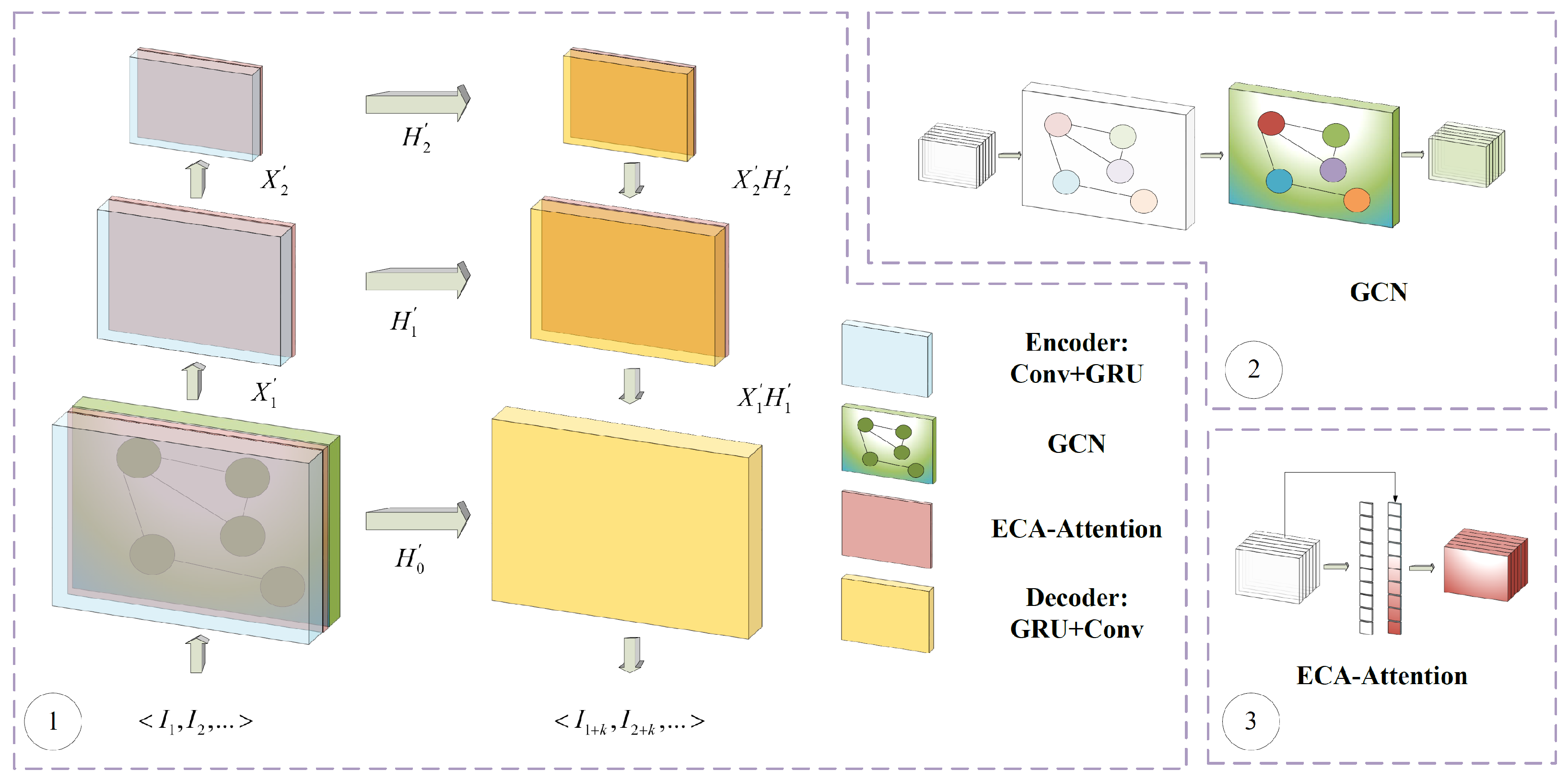
• The proposed method combines multiple refinements, including graph convolution, recurrent neural networks, convolutional neural networks, and attention mechanisms. We also adopt a hybrid loss function that includes mean square error (MSE) and difference structure similarity index measure (SSIM).
• We evaluate the model’s effectiveness using a time-space series prediction dataset based on radar echo data of cumulonimbus clouds. This dataset enables the rigorous evaluation of the model’s performance in predicting complex phenomena.

To provide a comprehensive understanding of the proposed method, we have organized the content of the following sections as follows: Section 2 provides a summary of recent developments in rainfall nowcasting technology. Section 3 presents the proposed method in detail. Section 4 describes the experimental settings used to evaluate the proposed method. Section 5 compares the performance of the proposed method with some state-of-the-art methods. Section 6 discusses the effectiveness of the proposed method. Finally, Section 7 concludes this manuscript and highlights future research directions.

2. Related Works

Currently, there are three primary deep network models utilized for rainfall prediction. The first model is the convolutional neural network (CNN), which processes input grid weather elements as images [12,17]. It performs feature learning through image filters and takes into account the spatial structure of the data. However, it has limitations in processing sequence data and is only suitable for fixed-length data. The second model is the recurrent neural network (RNN), which is commonly used in natural language processing [18]. It is flexible in processing sequence data through an autoregressive structure and is effective at learning in the time dimension. However, it loses the inherent spatial characteristics of grid data and has limited learning ability. The third approach combines CNN and RNN in various forms, allowing them to learn spatial and temporal features simultaneously. Previous studies have demonstrated the effectiveness of this approach [5,14]. Therefore, the selection of a deep network model for rainfall prediction depends on the specific characteristics of the input data and the desired output. CNNs are suitable for processing fixed-length data with spatial structure, while recurrent neural networks are better for processing sequence data with temporal structure. Combining these models can provide a more comprehensive approach to learning both spatial and temporal features, which is critical for accurate rainfall prediction.

The prediction of rainfall has undergone a significant evolution, progressing from pure RNN to Conv + RNN (a combination of CNN and RNN) to CNN. Shi et al. [5] proposed the pioneering ConvLSTM, which extends the idea of FC-LSTM by incorporating a convolutional structure in the input-to-state and state-to-state transitions. Multiple ConvLSTM layers were stacked to construct a precipitation adjacent to predicted end-to-end code-predict structure. The model consistently outperformed FC-LSTM when evaluated on both the moving MNIST dataset and the radar echo dataset. Souto Y M et al. [19] proposed a solution that combines recurrent networks with convolutional networks, using different channels to obtain the weights input to each prediction model. Their method improved accuracy by 50% for real weather datasets. Kim Y et al. [20] adopted a ConvLSTM network to predict the presence of rainfall and classify rainfall intensity. The experimental results showed that for longer-time predictions, lower rainfall intensities were predicted even if the rainfall was heavy, and for lighter rainfall intensities, the prediction time increased. Fang W et al. [21] designed the predictor (AttEF) module in the ConvLSTM encoder, allowing the encoder to encode all spatiotemporal information in a vector sequence. The experimental results demonstrated that the model could learn both short-term and long-term spatiotemporal dependencies, achieving the best performance on both datasets.

LSTM has a significant drawback of having a large number of parameters and is not well-suited for parallel computing training scenarios. To address this issue, Cho et al. [22] proposed a variant called gated recurrent unit (GRU). GRU combines the forget gate and the input gate into a single “update gate” and merges the cell state and the hidden state. This simplifies the model and reduces the number of parameters compared to the standard LSTM model. Additionally, GRU infers faster and requires less data to generalize.

Shi X et al. [14] argue that previous approaches have not focused on modifying the loop structure itself to solve the problem. Their model, TrajGRU, modifies the structure of loop connections and tests with different numbers of links to learn a more efficient connection structure. The improved HKO-7 dataset and moving MNIST dataset were used to evaluate seven models, with TrajGRU outperforming ConvLSTM. L. Tian et al. [23] proposed a disadvantage of ConvGRU, which uses mean squared error as a loss function, resulting in blurred extrapolated images and an inability to achieve the multi-modal and oblique intensities of real radar images. To address this issue, they proposed an adversarial model, GA-ConvGRU, consisting of a generator and a discriminator, which can produce more realistic and accurate inferences. Xie P et al. [24] argued that GA-ConvGRU has inherent shortcomings, where the generator and discriminator are easily trained in coordination, leading to training instability. They proposed the EBGAN-forecaster, which outperforms several existing models. Yu T et al. [25] argued that existing methods simply add additional parallel storage units outside the inner loop unit, and the different types of information are independent of one another. They introduced an axial attention memory module, ATMConvGRU, that can yield a stronger spatial-temporal feature correlation. Finally, Zhang et al. [26] proposed the M-ConvGRU model, which considers the interaction between input data and previous output data, merges the two states into ConvGRU neurons, and performs convolution-based gate preprocessing to capture contextual relations. For echo predictions longer than 1 h, M-ConvGRU outperforms ConvLSTM.

In addition to RNN, the academic community has also explored the use of CNN for rainfall prediction, with models such as U-Net, Smatunet, and Seresunet. In the Weather4cast competition, the RNN-based model won first place, while the U-Net-based model won second place. However, when using more parameters and additional weather variables as input, U-Net-based models achieve higher scores in spatial transfer learning. A U-Net model that combines a numerical model and a deep learning model was proposed, taking numerical data from the NWP system as input and then correcting the data via U-Net to improve the accuracy of the final prediction. Trebing K et al. [17] proposed SmaAt-UNet, which is equipped with an attention module and depthwise separable convolution based on the efficient convolutional neural network of U-Net architecture. The experimental results showed that SmaAt-UNet achieves comparable prediction performance to other U-Net models while requiring only one-fourth of the trainable parameters. Song K et al. [12] proposed SE-ResNet to distinguish moving/deformed rain regions from random noise regions. The input–output cross-entropy was used as a loss function to remove noise in radar images. The regressor integrates FCN and uses the attention mechanism and the IOU regression loss function. The experimental results showed that the algorithm outperforms RNN.

However, the above methods do not consider integrating the temporal dimension with the high-level semantic information in the image, which could help the model learn more accurate feature representations. Graph convolutional networks (GCNs) are capable of learning data with arbitrary graph structures and have been successfully applied to many tasks. For graph data, GCN can fuse the information of itself and its nearby nodes, making two connected nodes highly correlated. Kipf T N et al. [27] proposed a scalable semi-supervised learning method for graph structures that scale linearly in the number of graph edges, learning hidden layer representations that encode local graph structure and node features. Extensive experiments show that this method is significantly better than related methods. Wu Y et al. [28] proposed GCRN with a multi-convolution mechanism to tolerate the varying spatial correlations in actual precipitation, extending the central node and its adjacent rain gauges to capture more complex spatial features of precipitation. Comparing the model with another graph recurrent architecture, GCRN can use fewer parameters and significantly improve performance, outperforming the QPE models. Although GCN has many advantages, there is not much literature applied to rainfall prediction at present, so it has research significance.

From the perspective of spatio-temporal modeling, precipitation nowcasting and video prediction are essentially spatio-temporal sequence prediction problems, where both input and output are spatio-temporal sequences. Compared to the general standard goal, time series are more challenging because each sample of the data in the time series is not independent. The closer the two samples in time are, the more relevant they are. Therefore, common classifiers cannot be used to fit the data as they assume that the two samples are independent. Currently, research is focused on addressing this issue with time series problems.

Compared with the traditional time series prediction problem, meteorological data can be viewed as image data. Therefore, some studies have introduced a learnable convolution as an image feature extractor to extract the high-level semantic information of the image. This semantic information is then imported into the recurrent neural network for learning. Finally, the predicted features are decoded and up-sampled to obtain predicted image information. The model mainly adopts the encoder–decoder architecture for feature extraction and remapping. The slice of meteorological time series data in each space can be regarded as a kind of image data with uneven distribution. Convolutional layers are better at extracting features in Euclidean space due to the specific shape of their convolution kernels. Graph convolution has a strong ability to represent features. It can construct topological structure information of semantic features, map traditional image features to graph structure information, and build feature associations to achieve more accurate feature extraction.

This paper introduces the use of graph convolution to enhance the encoder–decoder model that is built using traditional CNN and RNN. The goal is to improve the learning ability of the model for time series data. Additionally, a low-parameter attention mechanism is adopted to optimize the feature distribution of the convolutional layer in the feature extraction and reconstruction stage of the model.

3. Methods

The proposed method contains three main structures: 1, an encoder–decoder network based on CNN and RNN; 2, an attention mechanism to enhance the feature extraction ability; and 3, a GCN layer to better build correlations between features. The structure diagram of the proposed GraphAT-NET is presented in Figure 1. In the following subsections, we introduce the mathematics and deployment of the details of the proposed method.

3.1. Trajectory GRU Structure

As presented in the ➀ part of Figure 1, the proposed method adopts RNN to build the correlation between time and radar data. The whole structure can be identified as a three-step encoding and decoding module. We assume the input radar data ($I_1$) are separated alone time dimension: $<I_1,I_2,\dots >$. Then the prediction task can be arranged as forecasting k steps based on the inputs: $<I_{1+k},I_{2+k},\dots >$. The task of rainfall prediction is defined as a sequence learning-predicting mission. The main algorithm we adopted in the proposed method can be defined as follows:

The observations into n layers of RNN: $H_t^1,H_t^2,\dots ,H_t^n=h\left(I_{t-J+1},I_{t-J+2},\dots ,I_t\right)$ (here, h indicates operating history information), and then use another n layer of RNNs to generate the predictions based on these encoded states: $\stackrel{⌢}{I}$_{t + 1}, $\stackrel{⌢}{I}$_{t + 2}, …, $\stackrel{⌢}{I}$_{t + K} = g($H_t^1$, $H_t^2$, …, $H_t^n$) (here, g indicates the gate operation of RNN). Based on the introduction above, we define the methods of trajectory GRU as follows:

$$\begin{array}{c}\hfill \begin{array}{cc}\hfill U_{t,}{V}_t& =\gamma (X_t^{{}^{\prime }},H_{t-1})\hfill \end{array}\end{array}$$

(1)

$$\begin{array}{c}\hfill \begin{array}{cc}\hfill Z_t& =\sigma (W_{xz}\times X_t^{{}^{\prime }}+\sum _{l=1}^L{W}_{hz}^l)\hfill \\ \hfill & \times warp(H_{t-1},U_{t,l},V_{t,l})\hfill \end{array}\end{array}$$

(2)

$$\begin{array}{c}\hfill \begin{array}{cc}\hfill R_t& =\sigma (W_{xr}\times X_t^{{}^{\prime }}+\sum _{l=1}^L{W}_{hr}^l)\hfill \\ \hfill & \times warp(H_{t-1},U_{t,l},V_{t,l})\hfill \end{array}\end{array}$$

(3)

$$\begin{array}{c}\hfill \begin{array}{cc}\hfill {H^{\prime }}_t& =f(W_{xh}\times X_t^{{}^{\prime }}+R_t)\hfill \\ \hfill & \circ (\sum _{l=1}^L{W}_{hh}^l\times warp(H_{t-1},U_{t,l},V_{t,l}))\hfill \end{array}\end{array}$$

(4)

$$\begin{array}{c}\hfill \begin{array}{cc}\hfill H_t& =(1-Z_t\circ {H^{\prime }}_t+Z_t)\circ H_{t-1}\hfill \end{array}\end{array}$$

(5)

Here, L is the total number of allowed links. $U_{t,}{V}_t\in {\mathbb{R}}^{L\times H\times W}$ are the flow fields that store the local connection structure generated by the structure generating network $\gamma$. And $W_{hz}^l,W_{hr}^l,W_{hh}^l$ are the weights for projecting the channels, which are implemented by $1\times 1$ convolutions. The $warp(H_{t-1},U_{t,l},V_{t,l})$ function selects the position pointed out by $U_{t,l},V_{t,l}$ from $H_{t-1}$ via the bilinear sampling kernel. If we denote $M=warp(I,U,V)$ where $M,I\in {}^{C\times H\times W}$ and $\mathrm{U},\mathrm{V}\in {}^{H\times W}$, we have:

$$\begin{array}{cc}\hfill M_{c,i,j}=& \sum _{m=1}^H\sum _{N=1}^W{I}_{c,m,n}max(0,1-\left|i+{\mathrm{V}}_{i,j}-m\right|)max(0,1-\left|j+{\mathrm{U}}_{i,j}-n\right|)\hfill \end{array}$$

(6)

The advantage of this framework is the ability to learn features through image sequences. However, radar images, as a complex data source, have features that cause problems.

3.2. GCN Structure

Radar images are generated from the echo signal of clouds. Cumulonimbus is related to humidity, wind, temperature, topography, etc. [29]. These matters constructed a chaos system. Thus, we need to insert nonlinear mapping components to build relationships within these features. GCN has been proven to be a network that can build the such relationship in irregular data. In this work, we embedded GCN layers in the proposed method to learn the features of cumulonimbus. The structure diagram is presented in the ➁ part of Figure 1. We introduce the GCN components in the following paragraphs:

First, we define the transition pattern of GCN as presented in Equation (7):

$$H^{(l+1)}=ReLU\left({\widehat{D}}^{-\frac{1}{2}}\widehat{A}{\widehat{D}}^{-\frac{1}{2}}{H}^{\left(l\right)}{W}^{\left(l\right)}\right)$$

(7)

Here, $\widehat{A}=A+I$ A is the adjacency matrix, I is the identity matrix, $H^{\left(l\right)}$ is the graph-level outputs, $H^{\left(0\right)}$ is the input X, $\widehat{D}$ is the diagonal node degree matrix of $\widehat{A}$, and $ReLU(·)$ is the ReLU activation function.

In this model, the GCN is embedded after the first convolutional RNN layer, and the features are reorganized, which balances the computational complexity and the effectiveness of the GCN. This part of the component is composed of two layers of GCNs, and the correlation between GCN and TrajGRU can be concluded as follows:

$$H_1=GCN\left(h_1\right)$$

(8)

Here, the input of the GCN layer is the state tensor of the first convolutional RNN layer.

To initialize the relations within features, we create a Gaussian distribution matrix as the adjacent matrix A. Then, we use the initialized weight matrix and bias matrix to transport and learn features during training. After the inner operations within the first layer of GCN, we use the ReLU activation function to enhance the nonlinear mapping capability of GCN. To avoid overfitting during training, we use dropout to randomly disable 50% of the neurons. After that, we use another GCN layer to compose the bottleneck structure. Finally, we have the enhanced stage tensor $H_1$.

3.3. ECA Attention Structure

The attention mechanism is an effective method to improve the feature extraction ability of deep neural networks. To further improve the convolutional layers in the encoder and decoder of the proposed method, we embed a lightweight attention layer after each convolutional layer. To reach the balance between performance and efficiency, we adopt efficient channel attention (ECA) attention in this method. The structure diagram is presented in the ➂ part of Figure 1, and the details of ECA are as follows:

First, we use adaptive average pooling to generate the channel-wise weight of the feature maps:

$$\mathbf{w}=Adaavgpool\left(X_t\right)$$

(9)

After that, we use two layers of 1D convolutional layers to enhance the relationships of channel weight:

$${\mathbf{w}}^{\prime }=Conv1D\left(\mathbf{w}\right)$$

(10)

Then, we use sigmoid activation function to enhance the nonlinear mapping ability of ${\mathbf{w}}^{\prime }$:

$${\mathbf{w}}^{″}=\sigma \left({\mathbf{w}}^{\prime }\right)$$

(11)

Finally, we use the inner product of ${\mathbf{w}}^{″}$ and input feature maps as the enhanced feature:

$$X_t^{{}^{\prime }}=({\mathbf{w}}^{″}\times X_t)$$

(12)

4. Experiment Settings

This section describes the experiment settings of this work, which evaluate the effectiveness of the proposed method using two datasets. The moving MNIST dataset is a benchmark for testing and evaluating prediction models. The second dataset is real-world time sequence data used to assess the prediction ability of the proposed method. These datasets are crucial for evaluating the proposed method and its potential applications.

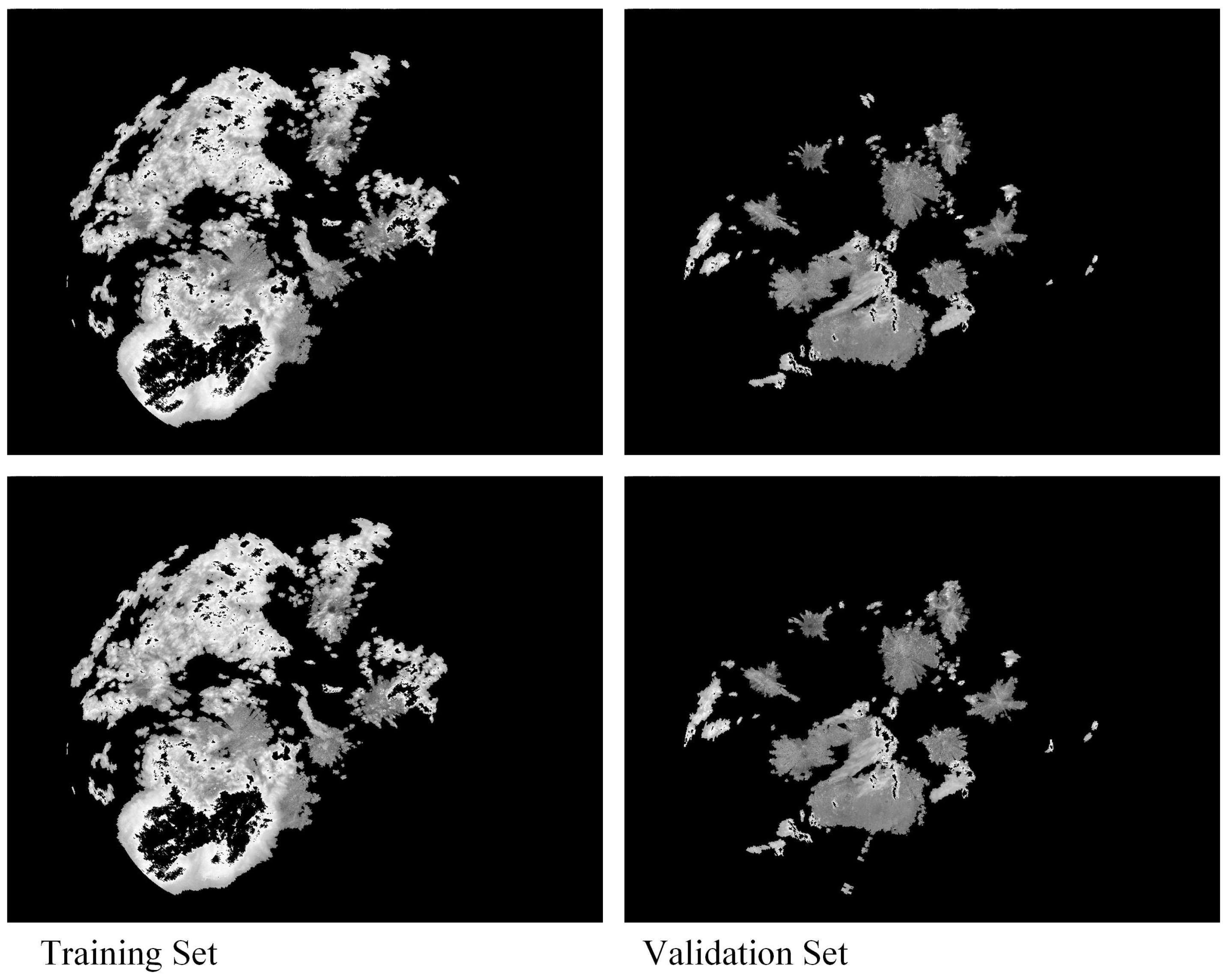
4.1. Dataset Information

Moving MNIST [16] is a handwriting digit dataset based on the MNIST dataset [30]. It consists of 10,000 sequences, each containing 20 frames with a size of $64\times 64$ pixels, where digits move inside each patch. The dataset is commonly used as a benchmark for testing and evaluating video prediction models due to its complexity and diversity. The moving MNIST dataset is generated by adding random motion blur with random speeds and directions to the MNIST digits. Examples of the moving MNIST dataset are presented in Figure 2.

The Guangxi constant altitude plan position indicating (GCAPPI) dataset is a high-time resolution record dataset of cumulonimbus cloud distribution in Guangxi province, China. The research area covers (102–114${}^{\circ }$ E, 19–28${}^{\circ }$ N). The experimental data consist of radar maps collected by 10 Doppler radars in Guangxi. The radar data are sampled and processed by the severe weather analysis and prediction system (SWAN) of the China Meteorological Administration to form a gridded reflectivity factor isosurface mosaic, with a horizontal resolution of $0.{01}^{\circ }\times 0.{01}^{\circ }$ and an altitude spectrum ranging from $0.5$ to $10.5$ km. In order to avoid ground interference and improve the reliability of data [2], the quality control algorithm was applied to remove isolated noise and ground echoes [31]. Specifically, the algorithm identified and removed echoes with low reflectivity values and those that were not contiguous with other echoes [32]. This step helped to reduce the impact of non-meteorological echoes on the analysis. We selected the radar maps from June 2019, with a time resolution of 6 min. The original radar echo data are stored in bin format as echo data with amplitudes ranging from −128 to 127. To better form image information, we rescale the amplitudes to the range of 0 to 255. In addition, to avoid noise and abnormal values affecting the feature extraction process, we use the Daubechies8 wavelet for filtering. This results in a radar echo image with a size of $1200\times 900$. The GCAPPI dataset contains a total of 7200 frames, which were separated into a 6:4 training set and testing set, i.e., the GCAPPI dataset includes a training set of 4320 frames and a validation set of 2880 frames. To improve the operation speed, we resized the radar map size to $256\times 256$. Examples of the GCAPPI dataset are presented in Figure 3.

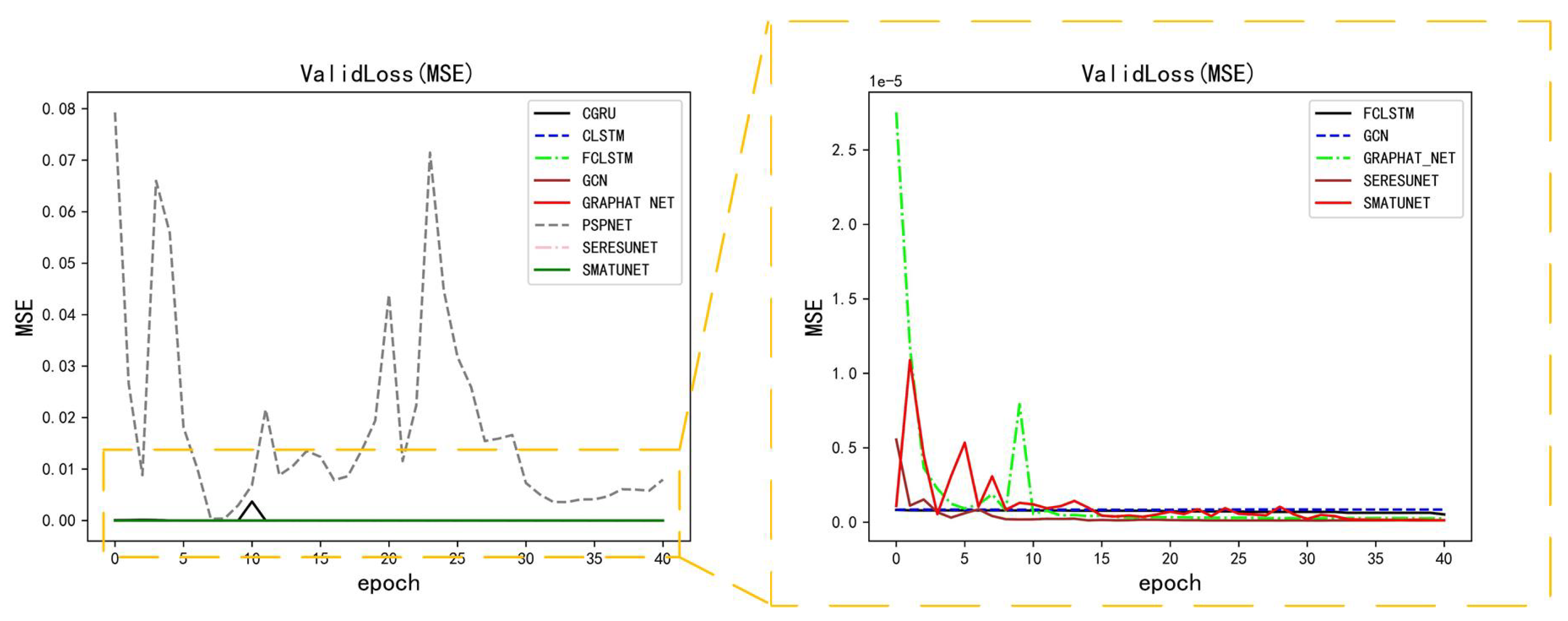
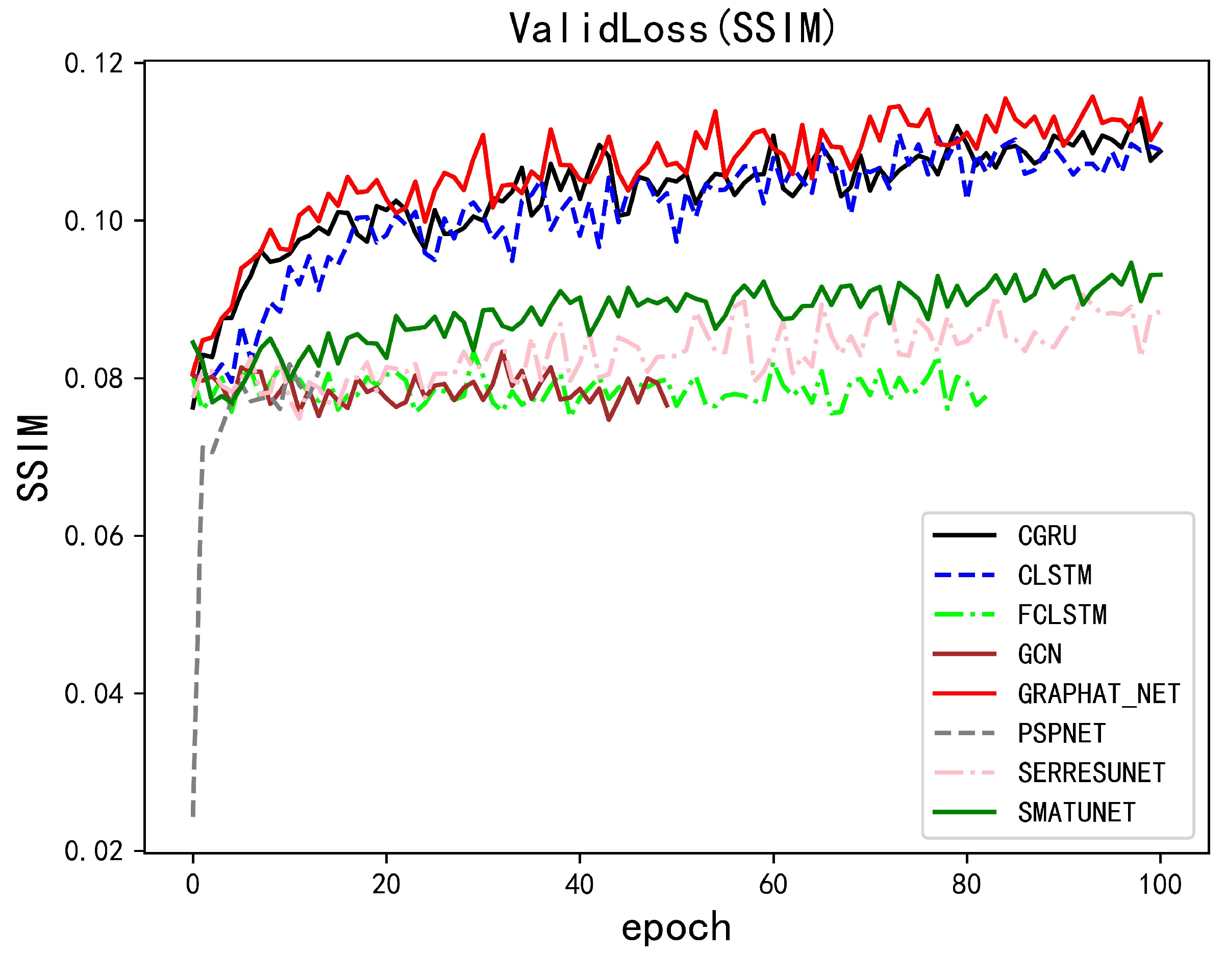
4.2. Evaluation Metrics

MSE (mean square error) is the root of the deviation between the observed value and the ground truth value divided by the number of observations and is used to measure the deviation [33]. The standardized mean-variance is based on calculating the ratio of the accuracy between the model to be evaluated and the model based on the mean. The value range of the standardized mean-variance is usually 0 to 1. The smaller the ratio, the better the model is than the mean-based prediction strategy. The standard error is very sensitive to very large or very small errors in a group of measurements, so the standard error can reflect the precision of the measurement well. Therefore, this paper adopts MSE as the evaluation method to evaluate the performance of each model.

$$MSE(x,y)=\frac{1}{n}\sum _{i=1}^n{(x-y)}^2$$

(13)

SSIM (structure similarity index measure) [34], is used to evaluate the similarity between the target image and the generated image. SSIM mainly concerns three indicators: luminance, contrast, and structure. First, luminance calculates the similarity between two patches; the closer two patches are, the larger luminance is. The definition of luminance is:

$$Luminance(x,y)=\frac{2{\mu }_x{\mu }_y}{{\mu }_x^2+{\mu }_y^2}$$

(14)

Here, $\mu$ indicates the average value of corresponding patch.

Second, contrast measures the distance between the texture of two patches; the definition of contrast is:

$$Contrast(x,y)=\frac{2{\sigma }_x{\sigma }_y}{{\sigma }_x^2+{\sigma }_y^2}$$

(15)

Here, $\sigma$ means the variance of corresponding patch.

Third, structure is the correlation between the pixel values in two patches. The more edges with the same position and direction two patches contain, the higher score is. The definition of structure is:

$$Structure(x,y)=\frac{{\sigma }_{xy}}{{\sigma }_x{\sigma }_y}$$

(16)

Finally, when we add weight($\omega$) among three indicators, we have:

$$\begin{array}{cc}\hfill SSIM(x,y)=& {\omega }_{L}Luminance(x,y)\hfill \\ \hfill & \times {\omega }_{C}Contrast(x,y)\hfill \\ \hfill & \times {\omega }_{S}Structure(x,y)\hfill \end{array}$$

(17)

Obviously, the larger SSIM is, the better the model predicts.

4.3. Training Details

The experiments were conducted on a hardware platform that contains an Intel i5-9400f CPU, 24 GB RAM, and GTX 1080Ti GPU. All of the code was programmed and executed in PyTorch 1.8.

As introduced above, two datasets are adopted in this work. And the size of moving MNIST and GCAPPI data varies from each other. Thus, to achieve a balance between performance and hard platform, we use different training settings:

Moving MNIST: In the moving MNIST experiment, the batch size is 8, the learning rate is $1\times {10}^{-4}$, the input is 10 frames, and the predict the next 10 frames. The total epoch is 100. We use Adam as the optimizer. We also use a learning rate scheduler to change the learning rate. The dynamic learning rate adjustment strategy we adopted in this experiment is ReduceLROnPlateau. As for training loss, we combine MSE loss with SSIM loss; the loss function is presented in Equation (18). In Equation (18), ${\widehat{I}}_{t+k}$ represents the ground truth and $I_{t+k}$ represents the sequence image predicted by the model. The loss function is mainly composed of the mean squared error (MSE) loss function and the structural similarity index (SSIM) loss function, which are added together and then divided by 2. This constrains the maximum value of the loss and improves training stability. To prevent overfitting, we adopted early stopping in the experiments, i.e., if the loss value does not decrease in 5 epochs, the training procedure will stop.

$$\begin{array}{cc}\hfill Loss=& \left(MSE\right({\stackrel{⌢}{I}}_{t+k}\hfill \end{array},I_{t+k})+(1-SSIM({\stackrel{⌢}{I}}_{t+k},I_{t+k}))/2)/2$$

(18)

GCAPPI dataset: In the GCAPPI experiment, we basically follow the same set of moving MNIST datasets. However, considering the size of GCAPPI dataset and the limitation of the hardware platform, we adjust the batch size to 1, and the amount of input frames and prediction frames is 4. We compare the performance of methods after 40 epochs of training.

5. Performance

This section aims to demonstrate the superiority of the proposed method by comparing it with several representative methods in the field. The comparison is conducted with respect to the following methods: LSTM with fully connected layers (FC-LSTM), GCNnet, PSPNet, Seresunet, Smatunet, ConvLstm, and ConvGRU. These methods have been widely used in previous studies and are considered benchmarks for evaluating prediction models.

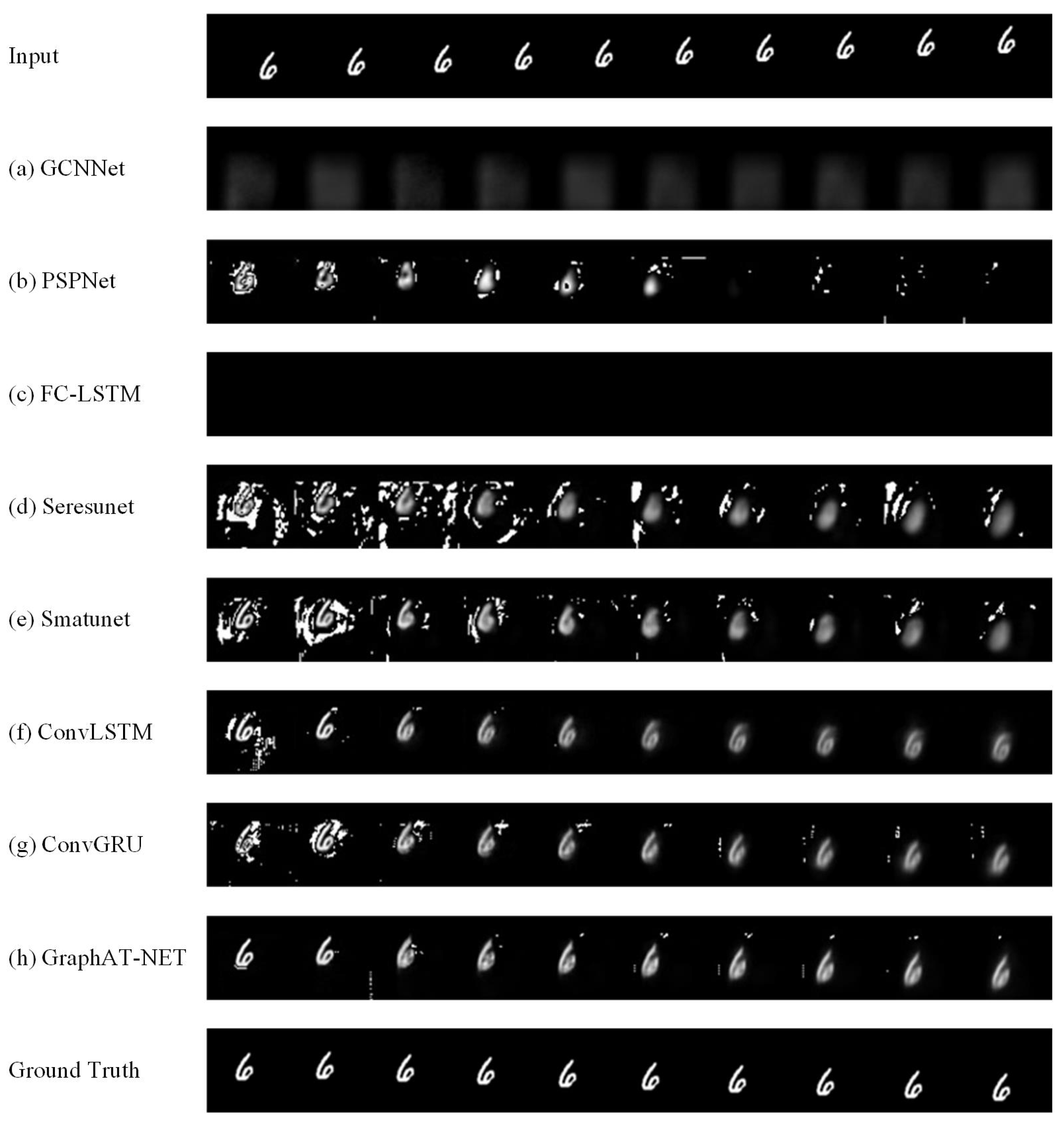
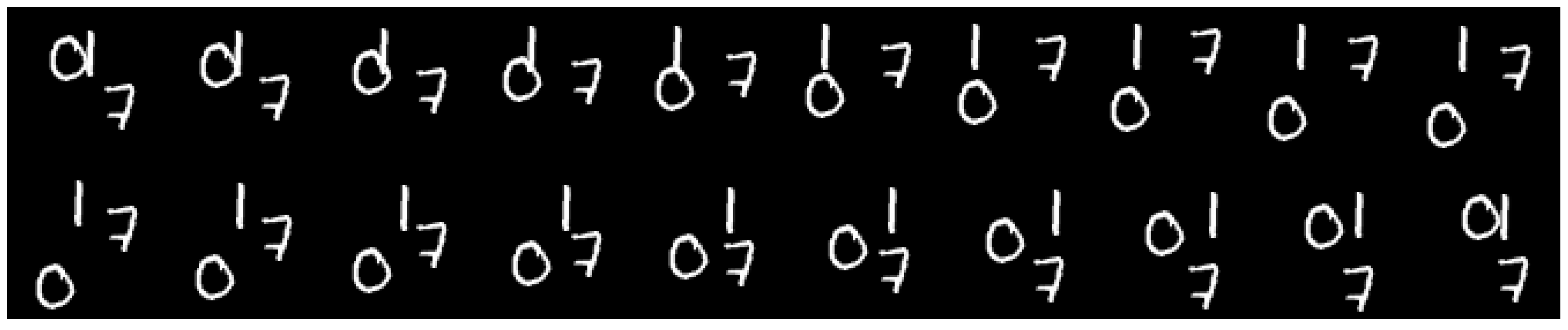
5.1. Performance of Methods on Moving-MNIST Dataset

We present the experiment results of the moving MNIST dataset in

Table 1. Comparison of the proposed model with other models based on the moving MNIST dataset (Vali Loss is short for validation loss).

Methods	MSE	SSIM	Vali Loss
GCNNet	$7.43\times {10}^{-3}$	$8.33\times {10}^{-4}$	$4.83\times {10}^{-1}$
PSPNet	$7.00\times {10}^{-3}$	$8.17\times {10}^{-4}$	$4.83\times {10}^{-1}$
FC-LSTM	$6.49\times {10}^{-3}$	$8.33\times {10}^{-4}$	$4.82\times {10}^{-1}$
Seresunet	$4.44\times {10}^{-3}$	$9.45\times {10}^{-4}$	$4.79\times {10}^{-1}$
Smatunet	$3.58\times {10}^{-3}$	$9.46\times {10}^{-4}$	$4.78\times {10}^{-1}$
ConvLSTM	$1.49\times {10}^{-3}$	$1.10\times {10}^{-3}$	$4.73\times {10}^{-1}$
ConvGRU	$41.39\times {10}^{-3}$	$1.09\times {10}^{-3}$	$4.74\times {10}^{-1}$
GraphAT-Net	$\mathbf{1}.\mathbf{23}\times {\mathbf{10}}^{-\mathbf{3}}$	$\mathbf{1}.\mathbf{12}\times {\mathbf{10}}^{-\mathbf{3}}$	$\mathbf{4}.\mathbf{72}\times {\mathbf{10}}^{-\mathbf{1}}$

, sorted by MSE values. To more specifically present the advantage of the proposed method, we calculated the increased percentage ($ip$) of corresponding indicators (with $ip=|a-b|/b$). For MSE, the increase percentages are ConvGRU: 11.51%; ConvLSTM: 17.45%; Smatunet: 65.64%; Seresunet: 72.30%; FC-LSTM: 91.05%; PSPNet: 82.43%; GCNNet: 83.45%. As for SSIM, the increase percentages are: ConvGRU: 3.47%; ConvLSTM: 2.14%; Smatunet: 15.84%; Seresunet: 15.93%; FC-LSTM: 25.88%; PSPNet: 27.31%; and GCNNet: 25.89%.

In addition, we present the performance of different models on the moving MNIST dataset in Figure 4 and Figure 5, respectively. Limited by the ability of different models, PSPNet, GCN, and FC-LSTM triggered the early stopping mechanism. Evidently, GraphAT-NET outperforms the other models in both the mean squared error (MSE) and structural similarity index (SSIM) metrics. Firstly, GCN performs the worst, possibly because it cannot extract spatio-temporal feature information from sequence data alone. Additionally, fully CNN-based models such as PSPNet, Seresunet, and Smatunet, which use CNN to construct spatio-temporal feature correlation information, still do not achieve as high prediction accuracy as models that combine CNN and RNN. Furthermore, as a typical machine learning method, FC-LSTM is not sufficient to learn feature representations from the moving MNIST dataset. Comparing the models, Convlstm, Convgru, and the proposed model show significantly improved accuracy compared to other models. This may be because CNN can extract feature information from images, and RNN can build spatio-temporal feature information based on the correlation between image features. Additionally, Table 1 shows that the proposed model achieves the highest accuracy.

To better demonstrate the advantages of the proposed model, we display the visualization results in Figure 6, following the order of Table 1. It is evident that GCN can only achieve fuzzy predictions of the region, which is consistent with the previous speculation that an image-sensitive CNN structure is necessary to extract image details. Notably, FC-LSTM learned nothing but the background and failed to make any predictions in the moving MNIST dataset. Furthermore, in the visualization results of PSPNet, Seresunet, and Smatunit in Figure 6, the short-term prediction results are better and clearer, while the long-term distribution becomes fuzzy and more disturbed. This may be because it is difficult for the model to build the spatio-temporal feature association relationship, making it challenging for the model built only by CNN to make long-term predictions. Compared with ConvLSTM, ConvGRU, and the proposed model results, it is apparent that the architecture built by CNN and RNN can better extract spatio-temporal feature information and make more accurate predictions. However, the prediction results of ConvLSTM and ConvGRU still contain a lot of interference, which affects the prediction results. Additionally, it can be observed that the prediction accuracy of all models decreases with time. Nevertheless, it is evident from the visualization results that the proposed model achieves the best prediction accuracy.

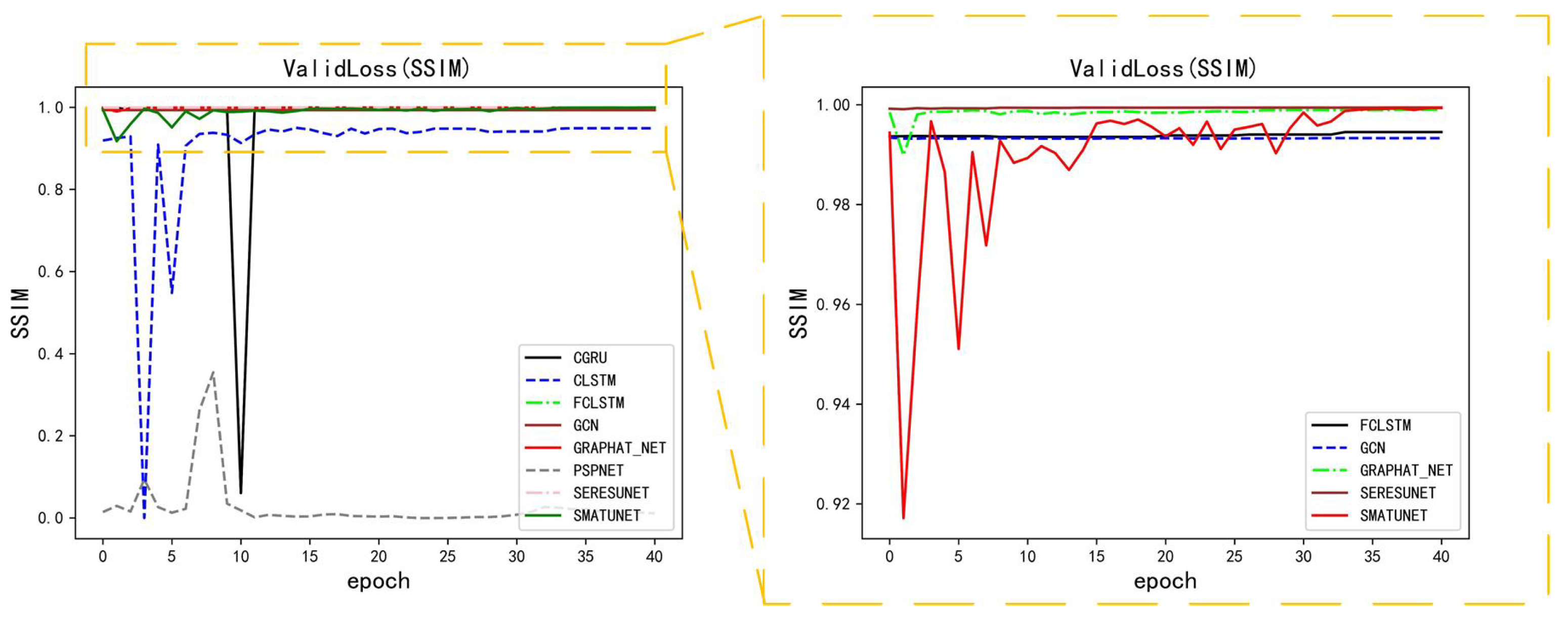
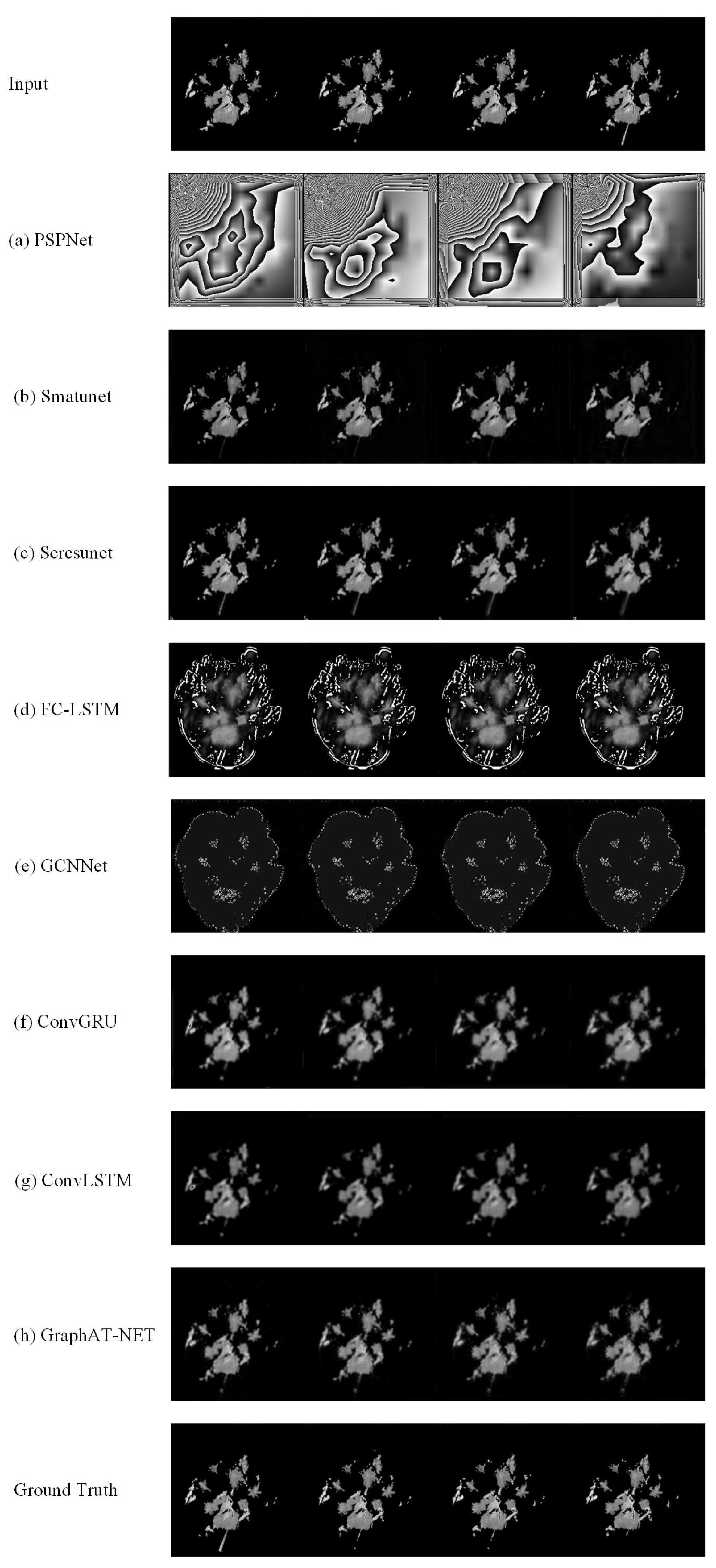
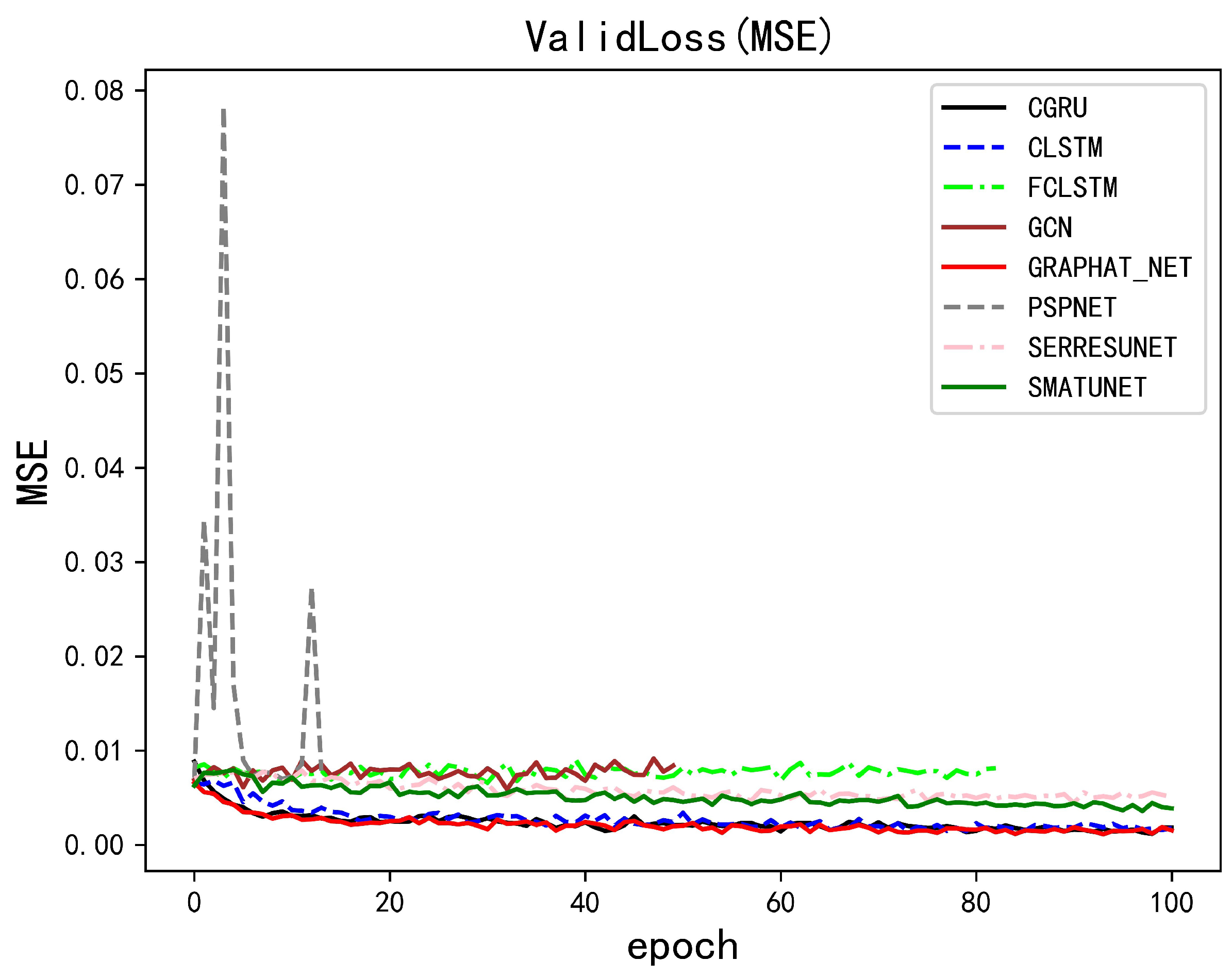
5.2. Performance of Methods on GCAPPI Dataset

Table 2. Comparison of the proposed model with other models based on the GCAPPI dataset (Vali Loss is short for validation loss).

Methods	MSE	SSIM	Vali Loss
PSPNet	$3.16\times {10}^{-4}$	$3.55\times {10}^{-1}$	$4.99\times {10}^{-1}$
Smatunet	$1.54\times {10}^{-6}$	$9.89\times {10}^{-1}$	$\mathbf{4}.\mathbf{98}\times {\mathbf{10}}^{-\mathbf{1}}$
Seresunet	$1.21\times {10}^{-6}$	$9.94\times {10}^{-1}$	$\mathbf{4}.\mathbf{98}\times {\mathbf{10}}^{-\mathbf{1}}$
FC-LSTM	$8.24\times {10}^{-7}$	$9.94\times {10}^{-4}$	$\mathbf{4}.\mathbf{98}\times {\mathbf{10}}^{-\mathbf{1}}$
GCNNet	$8.32\times {10}^{-7}$	$9.93\times {10}^{-1}$	$\mathbf{4}.\mathbf{98}\times {\mathbf{10}}^{-\mathbf{1}}$
ConvGRU	$2.63\times {10}^{-7}$	$9.98\times {10}^{-1}$	$\mathbf{4}.\mathbf{98}\times {\mathbf{10}}^{-\mathbf{1}}$
ConvLSTM	$2.20\times {10}^{-7}$	$9.50\times {10}^{-1}$	$\mathbf{4}.\mathbf{98}\times {\mathbf{10}}^{-\mathbf{1}}$
GraphAT-Net	$\mathbf{1}.\mathbf{98}\times {\mathbf{10}}^{-\mathbf{7}}$	$\mathbf{9}.\mathbf{99}\times {\mathbf{10}}^{-\mathbf{1}}$	$\mathbf{4}.\mathbf{98}\times {\mathbf{10}}^{-\mathbf{1}}$

presents the performance of methods on the GCAPPI dataset, sorted according to the MSE value. As shown in Table 2, the proposed method outperforms others on both MSE and SSIM. For MSE values, the proposed method has $ip$ over other methods with: ConvLSTM: 10.92%; ConvGRU: 24.72%; FC-LSTM: 76.01%; GCNNet: 76.23%; Seresunet: 83.59%; Smatunet: 87.18%; and PSPNet: 99.94%. As for the results of SSIM, the proposed method outperforms other methods with: ConvLSTM: 4.92%; ConvGRU: 0.08%; FC-LSTM: 0.45%; GCNNet: 0.57%; Seresunet: 0.50%; Smatunet: 0.99%; and PSPNet: 64.51%. In the experiment on real-world data, pure CNN methods such as PSPNet, Smatunet, and Seresunet perform worse than methods based on GCN and RNN. This is because of their lack of spatio-temporal feature extraction ability. The results of other methods in Table 2 also verify that the combination of CNN, RNN, and GCN can help methods to extract the distributions of cumulonimbus clouds along the time dimension. Moreover, the proposed method performs the best on real-world data.

We demonstrate the performance of the compared algorithms on the CAPPI dataset over time in Figure 7 and Figure 8. Due to hardware limitations, the training epoch of CAPPI is 40. Early stopping is not used in the CAPPI dataset experiment. It can be observed that PSPNet is ineffective in training on the CAPPI dataset. To better illustrate the training details, we excluded the loss curves of PSPNet, CLSTM, and CGRU and displayed the detailed plots on the right side of Figure 7 and Figure 8. It can be seen that GCN, FC-LSTM, SERESUNET, SMATUNET, and GraphAT-NET perform similarly at the end of training, making it difficult to compare them intuitively based on loss values.

We present the visual results of corresponding methods in Figure 9. We analyze the results of Figure 9 row by row. Firstly, the visual results of PSPNet show the worst performance on both indicators and visual results, making them unacceptable. Secondly, the visual results of Smatunet and Seresunet learn the prediction task as a segmentation task. This is evident from the minimal differences in contour and details, indicating that these models only learn spatial distribution rather than temporal correlations. Thirdly, FC-LSTM can make basic predictions of the distribution of cumulonimbus clouds, but there are still many noise interferences in the results. Fourthly, the unsatisfactory performance of pure GCN is due to its inability to study spatial distributions. Fifthly, comparing the results of ConvGRU and ConvLSTM, both methods have predicted vague spatio-temporal distributions. Lastly, the proposed method generates the most accurate predictions, with clearer details than those of ConvGRU and ConvLSTM results.

6. Ablation Study

In this section, we analyze the effectiveness of the modules in the proposed method. We conduct experiments on the GCAPPI dataset to discuss the validity of the corresponding modules. The details are presented in the following sections.

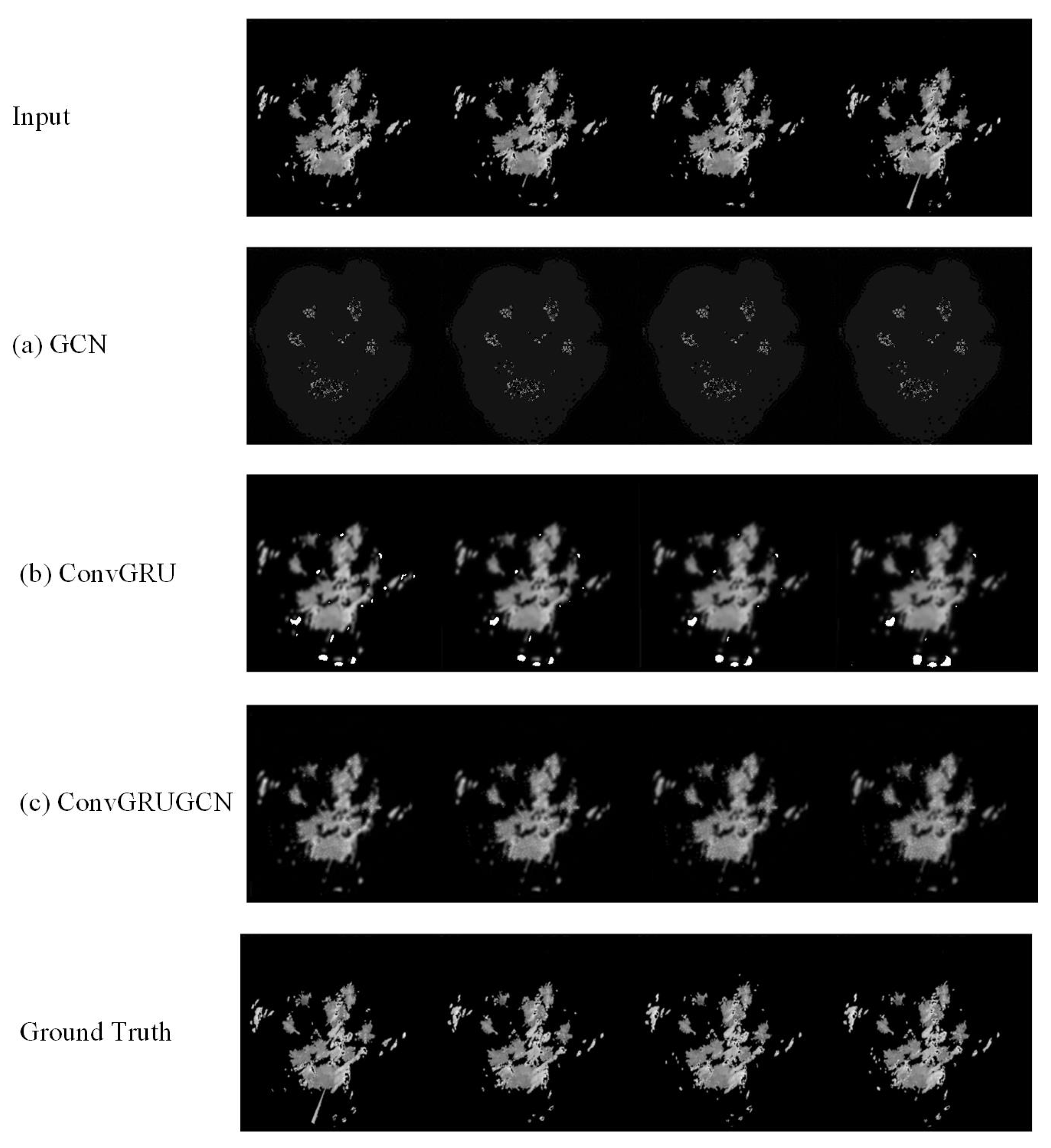
6.1. Effectiveness of GCN

To validate the effectiveness of the GCN module, we conducted experiments among GCNNet, ConvGRU, ConvGRU + GCNNet, and GraphAT-Net. The purpose of this experiment is to evaluate the contribution of the GCN module to the performance of GraphAT-Net. As shown in

Table 3. Performance of methods in ablation study on GCN module (Vali Loss is short for validation loss).

Methods	MSE	SSIM	Vali Loss
GCNNet	$8.32\times {10}^{-7}$	$9.93\times {10}^{-1}$	$\mathbf{4}.\mathbf{98}\times {\mathbf{10}}^{-\mathbf{1}}$
ConvGRU	$2.63\times {10}^{-7}$	$9.98\times {10}^{-1}$	$\mathbf{4}.\mathbf{98}\times {\mathbf{10}}^{-\mathbf{1}}$
ConvGRU + GCN	$2.34\times {10}^{-7}$	$9.98\times {10}^{-1}$	$\mathbf{4}.\mathbf{98}\times {\mathbf{10}}^{-\mathbf{1}}$
GraphAT-Net	$\mathbf{1}.\mathbf{98}\times {\mathbf{10}}^{-\mathbf{7}}$	$\mathbf{9}.\mathbf{99}\times {\mathbf{10}}^{-\mathbf{1}}$	$\mathbf{4}.\mathbf{98}\times {\mathbf{10}}^{-\mathbf{1}}$

, ConvGRU with GCN increased about 10.9% on MSE and showed the same performance on SSIM. This indicates that GCNNet could enhance the model to learn more accurate features. Specifically, the GCN module can capture the spatial dependencies among the input data and propagate the information to the subsequent layers, which leads to more accurate predictions. To better illustrate the enhancement, we present visual results in Figure 10. As shown in Figure 10, the results of pure GCN are still unreadable, while ConvGRU + GCN performs much better than ConvGRU. This verifies the effectiveness of GCN as an embedded module in the CNN+RNN-based framework. Specifically, the GCN module can effectively capture the spatial correlations in the input data and enhance the feature representation of the model, which leads to more accurate predictions. The experimental results demonstrate that the GCN module can effectively enhance the feature representation of the model and improve the accuracy of the predictions. Therefore, the GCN module is a valuable addition to the proposed method and can be used to improve the performance of other CNN + RNN-based models.

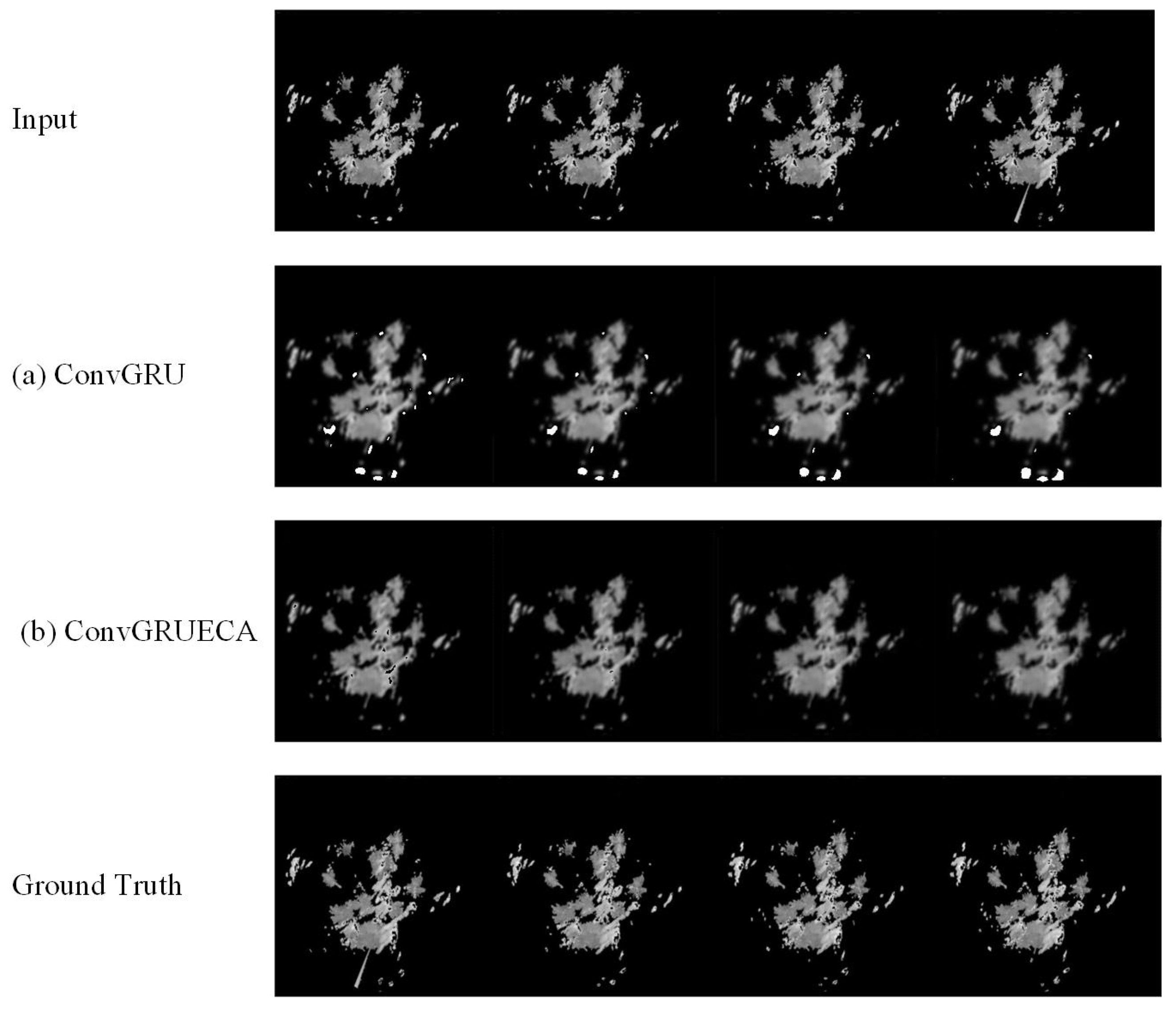
6.2. Effectiveness of ECA

In this subsection, we discuss the effectiveness of the ECA module. We present the experimental results in

Table 4. Performance of methods in ablation study on ECA module (Vali Loss is short for validation loss).

Methods	MSE	SSIM	Vali Loss
ConvGRU	$2.63\times {10}^{-7}$	$9.98\times {10}^{-1}$	$\mathbf{4}.\mathbf{98}\times {\mathbf{10}}^{-\mathbf{1}}$
ConvGRU + ECA	$2.12\times {10}^{-7}$	$9.98\times {10}^{-1}$	$\mathbf{4}.\mathbf{98}\times {\mathbf{10}}^{-\mathbf{1}}$
GraphAT-Net	$\mathbf{1}.\mathbf{98}\times {\mathbf{10}}^{-\mathbf{7}}$	$\mathbf{9}.\mathbf{99}\times {\mathbf{10}}^{-\mathbf{1}}$	$\mathbf{4}.\mathbf{98}\times {\mathbf{10}}^{-\mathbf{1}}$

and the visual results in Figure 11. The purpose of this experiment is to evaluate the contribution of the ECA module to the performance of the proposed method.

Table 4 shows that the ECA module helps ConvGRU improve by about 19.28% on MSE. This indicates that the ECA module can effectively enhance the feature representation of the model. Specifically, the ECA module can selectively emphasize informative features and suppress irrelevant ones, which leads to more accurate predictions. To better illustrate the effectiveness of the ECA module, we present visual results in Figure 11. As shown in Figure 11, the details of the ConvGRU+ECA results are more accurate than those of the ConvGRU results. In particular, the ConvGRU+ECA results have clearer boundaries and more accurate shapes, which indicates that the ECA module can effectively capture the spatio-temporal correlations in the input data. In summary, the experimental results demonstrate that the ECA module can effectively enhance the feature representation of the model and improve the accuracy of the predictions. Therefore, the ECA module is a valuable addition to the proposed method and can be used to improve the performance of other CNN+RNN-based models.

7. Conclusions

The proposed method utilizes a deep learning model combining CNN, GCN, RNN, the attention mechanism, and refined loss has demonstrated superior performance compared to other methods on both the moving MNIST dataset and real-world radar echo data. In the moving MNIST experiment, GraphAT-NET outperformed other methods with a 59.12% reduction in MSE and a 16.26% improvement in SSIM. The effectiveness of the proposed model was further confirmed through visualization results on the moving MNIST dataset. In the GCAPPI experiment, GraphAT-NET also exhibited an average increase of 65.40% in MSE and a 10.29% increase in SSIM. Additionally, the visualization results demonstrated that the proposed method outperformed other methods in terms of prediction accuracy and distribution detail. To analyze the effectiveness of different modules in GraphAT-NET, an ablation study was conducted. The study revealed that the GCN module facilitated the learning of complex feature relationships, resulting in an average 10.09% improvement in MSE. Furthermore, the ECA module enhanced accuracy, with a 19.28% improvement in MSE. Based on these results, we believe that the proposed GraphAT-NET method has the potential to improve the prediction of cumulonimbus cloud distribution. However, it is important to note that predicting cumulonimbus clouds is just the first step in the process of rainfall nowcasting. Our future work will focus on establishing connections between radar echo data and actual rainfall information, which will enable us to generate end-to-end predictions.

References

1. Collier, C.G. Developments in radar and remote-sensing methods for measuring and forecasting rainfall. Philos. Trans. R. Soc. A 2002, 360, 1345–1361. [Google Scholar] [CrossRef]
2. DALEZIOS, N.R. Digital processing of weather radar signals for rainfall estimation. Int. J. Remote Sens. 1990, 11, 1561–1569. [Google Scholar] [CrossRef]
3. Michaelides, S.; Levizzani, V.; Anagnostou, E.; Bauer, P.; Kasparis, T.; Lane, J. Precipitation: Measurement, remote sensing, climatology and modeling. Atmos. Res. 2009, 94, 512–533. [Google Scholar] [CrossRef]
4. Ghaemi, E.; Kavianpour, M.; Moazami, S.; Hong, Y.; Ayat, H. Uncertainty analysis of radar rainfall estimates over two different climates in Iran. Int. J. Remote Sens. 2017, 38, 5106–5126. [Google Scholar] [CrossRef]
5. Shi, X.; Chen, Z.; Wang, H.; Yeung, D.; Wong, W.; Woo, W. Convolutional LSTM Network: A Machine Learning Approach for Precipitation Nowcasting. In Proceedings of the Advances in Neural Information Processing Systems 28: Annual Conference on Neural Information Processing Systems 2015, Montreal, QC, Canada, 7–12 December 2015; pp. 802–810. [Google Scholar]
6. Peng, W.; Alan, S.; Lao, S.; Edel, O.; Yunxiang, L.; Noel, O. Short-term rainfall nowcasting: Using rainfall radar imaging. In Proceedings of the Eurographics Ireland 2009: The 9th Irish Workshop on Computer Graphics, Dublin, Ireland, 11 December 2009. [Google Scholar]
7. Scarchilli, G.; Gorgucci, V.; Chandrasekar, V.; Dobaie, A. Self-consistency of polarization diversity measurement of rainfall. IEEE Trans. Geosci. Remote Sens. 1996, 34, 22–26. [Google Scholar] [CrossRef]
8. Suhartono; Faulina, R.; Lusia, D.A.; Otok, B.W.; Sutikno; Kuswanto, H. Ensemble method based on ANFIS-ARIMA for rainfall prediction. In Proceedings of the 2012 International Conference on Statistics in Science, Business and Engineering (ICSSBE), Langkawi, Malaysia, 10–12 September 2012; pp. 1–4. [Google Scholar] [CrossRef]
9. Tang, L.; Hossain, F. Understanding the Dynamics of Transfer of Satellite Rainfall Error Metrics From Gauged to Ungauged Satellite Gridboxes Using Interpolation Methods. IEEE J. Sel. Top. Appl. Earth Obs. Remote Sens. 2011, 4, 844–856. [Google Scholar] [CrossRef]
10. Horn, B.K.P.; Schunck, B.G. Determining Optical Flow. Artif. Intell. 1981, 17, 185–203. [Google Scholar] [CrossRef]
11. Krizhevsky, A.; Sutskever, I.; Hinton, G.E. ImageNet classification with deep convolutional neural networks. Commun. ACM 2017, 60, 84–90. [Google Scholar] [CrossRef]
12. Song, K.; Yu, X.; Gu, Z.; Zhang, W.; Yang, G.; Wang, Q.; Xu, C.; Liu, J.; Liu, W.; Shi, C.; et al. Deep Learning Prediction of Incoming Rainfalls: An Operational Service for the City of Beijing China. In Proceedings of the 2019 International Conference on Data Mining Workshops, ICDM Workshops 2019, Beijing, China, 8–11 November 2019; pp. 180–185. [Google Scholar]
13. Sønderby, C.K.; Espeholt, L.; Heek, J.; Dehghani, M.; Oliver, A.; Salimans, T.; Agrawal, S.; Hickey, J.; Kalchbrenner, N. MetNet: A Neural Weather Model for Precipitation Forecasting. arXiv 2020, arXiv:2003.12140. [Google Scholar]
14. Shi, X.; Gao, Z.; Lausen, L.; Wang, H.; Yeung, D.; Wong, W.; Woo, W. Deep Learning for Precipitation Nowcasting: A Benchmark and A New Model. In Proceedings of the Advances in Neural Information Processing Systems 30: Annual Conference on Neural Information Processing Systems 2017, Long Beach, CA, USA, 4–9 December 2017; pp. 5617–5627. [Google Scholar]
15. Wang, D.; Zhang, C.; Han, M. FIAD net: A Fast SAR ship detection network based on feature integration attention and self-supervised learning. Int. J. Remote Sens. 2022, 43, 1485–1513. [Google Scholar] [CrossRef]
16. Srivastava, N.; Mansimov, E.; Salakhutdinov, R. Unsupervised Learning of Video Representations using LSTMs. In Proceedings of the 32nd International Conference on Machine Learning, ICML 2015, Lille, France, 6–11 July 2015; Volume 37, pp. 843–852. [Google Scholar]
17. Trebing, K.; Stanczyk, T.; Mehrkanoon, S. SmaAt-UNet: Precipitation nowcasting using a small attention-UNet architecture. Pattern Recognit. Lett. 2021, 145, 178–186. [Google Scholar] [CrossRef]
18. Mikolov, T.; Karafiát, M.; Burget, L.; Cernocký, J.; Khudanpur, S. Recurrent neural network based language model. In Proceedings of the INTERSPEECH 2010, 11th Annual Conference of the International Speech Communication Association, Chiba, Japan, 26–30 September 2010; pp. 1045–1048. [Google Scholar]
19. Souto, Y.M.; Porto, F.; de Carvalho Moura, A.M.; Bezerra, E. A Spatiotemporal Ensemble Approach to Rainfall Forecasting. In Proceedings of the 2018 International Joint Conference on Neural Networks, IJCNN 2018, Rio de Janeiro, Brazil, 8–13 July 2018; pp. 1–8. [Google Scholar] [CrossRef]
20. Kim, Y.; Hong, S. Very Short-term Prediction of Weather Radar-Based Rainfall Distribution and Intensity Over the Korean Peninsula Using Convolutional Long Short-Term Memory Network. Asia-Pac. J. Atmos. Sci. 2022, 58, 489–506. [Google Scholar] [CrossRef]
21. Fang, W.; Pang, L.; Yi, W.N.; Sheng, V.S. AttEF: Convolutional LSTM Encoder-Forecaster with Attention Module for Precipitation Nowcasting. Intell. Autom. Soft Comput. 2021, 30, 453–466. [Google Scholar] [CrossRef]
22. Chung, J.; Gülçehre, Ç.; Cho, K.; Bengio, Y. Empirical Evaluation of Gated Recurrent Neural Networks on Sequence Modeling. arXiv 2014, arXiv:1412.3555. [Google Scholar]
23. Tian, L.; Li, X.; Ye, Y.; Xie, P.; Li, Y. A Generative Adversarial Gated Recurrent Unit Model for Precipitation Nowcasting. IEEE Geosci. Remote Sens. Lett. 2020, 17, 601–605. [Google Scholar] [CrossRef]
24. Xie, P.; Li, X.; Ji, X.; Chen, X.; Chen, Y.; Liu, J.; Ye, Y. An Energy-Based Generative Adversarial Forecaster for Radar Echo Map Extrapolation. IEEE Geosci. Remote Sens. Lett. 2022, 19, 1–5. [Google Scholar] [CrossRef]
25. Yu, T.; Kuang, Q.; Yang, R. ATMConvGRU for Weather Forecasting. IEEE Geosci. Remote Sens. Lett. 2022, 19, 1–5. [Google Scholar] [CrossRef]
26. He, W.; Xiong, T.S.; Wang, H.; He, J.X.; Ren, X.Y.; Yan, Y.L.; Tan, L.Y. Radar Echo Spatiotemporal Sequence Prediction Using an Improved ConvGRU Deep Learning Model. Atmosphere 2022, 13, 88. [Google Scholar] [CrossRef]
27. Kipf, T.N.; Welling, M. Semi-Supervised Classification with Graph Convolutional Networks. In Proceedings of the 5th International Conference on Learning Representations, ICLR 2017, Toulon, France, 24–26 April 2017. [Google Scholar]
28. Wu, Y.; Tang, Y.; Yang, X.; Zhang, W.; Zhang, G. Graph Convolutional Regression Networks for Quantitative Precipitation Estimation. IEEE Geosci. Remote Sens. Lett. 2021, 18, 1124–1128. [Google Scholar] [CrossRef]
29. Markner-Jäger, B. Meteorology and Climatology. In Technical English for Geosciences; Springer: Berlin/Heidelberg, Germany, 2008; pp. 156–158. [Google Scholar] [CrossRef]
30. LeCun, Y.; Bottou, L.; Bengio, Y.; Haffner, P. Gradient-based learning applied to document recognition. Proc. IEEE 1998, 86, 2278–2324. [Google Scholar] [CrossRef]
31. Han, F.; Wo, W. Design and Implementation of SWAN2.0 Platform. J. Appl. Meteorol. Sci. 2016, 29, 25–34. [Google Scholar]
32. Wu, T.; Wan, Y.; Wo, W.; Leng, L. Design and Application of Radar Reflectivity Quality Control Algorithm in SWAN. Meterol. Sci. Technol. 2013, 41, 809. [Google Scholar]
33. Chai, T.; Draxler, R.R. Root mean square error (RMSE) or mean absolute error (MAE)?—Arguments against avoiding RMSE in the literature. Geosci. Model Dev. 2014, 7, 1247–1250. [Google Scholar] [CrossRef]
34. Wang, Z.; Bovik, A.C.; Sheikh, H.R.; Simoncelli, E.P. Image quality assessment: From error visibility to structural similarity. IEEE Trans. Image Process. 2004, 13, 600–612. [Google Scholar] [CrossRef] [PubMed]
Figure 1. Framework of GraphAT-NET (➀ is the overall architecture of the proposed model; ➁ is the structure diagram of GCN structure; and ➂ is the structure diagram of ECA-attention).
Atmosphere 14 01506 g001
Figure 2. Examples of Moving MNIST.
Atmosphere 14 01506 g002
Figure 3. Examples of GCAPPI dataset (the brightness in figure represents the radar echo signal, which represents the thickness of the cloud).
Atmosphere 14 01506 g003
Figure 4. The change of MSE loss value for different methods.
Atmosphere 14 01506 g004
Figure 5. The change of SSIM loss value for different methods.
Atmosphere 14 01506 g005
Figure 6. Performance of methods on moving MNIST dataset.
Atmosphere 14 01506 g006
Figure 7. The change of MSE loss value for different methods.
Atmosphere 14 01506 g007
Figure 8. The change of SSIM loss value for different methods.
Atmosphere 14 01506 g008
Figure 9. Performance of methods on GCAPPI dataset.
Atmosphere 14 01506 g009
Figure 10. Visual results of ablation study on GCN module.
Atmosphere 14 01506 g010
Figure 11. Visual results of ablation study on ECA module.
Atmosphere 14 01506 g011