Article

Effects of Typhoon Chanthu on Marine Chlorophyll a, Temperature and Salinity

1
Marine Science and Technology College, Zhejiang Ocean University, Zhoushan 316022, China
2
State Key Laboratory of Hydroscience and Engineering, Tsinghua University, Beijing 100084, China
3
College of Marine Science and Technology, Hainan Tropical Ocean University, Sanya 572022, China
*
Author to whom correspondence should be addressed.
Atmosphere 2023, 14(10), 1505; https://doi.org/10.3390/atmos14101505
Submission received: 31 July 2023 / Revised: 5 September 2023 / Accepted: 27 September 2023 / Published: 28 September 2023
(This article belongs to the Section Meteorology)

Abstract

:
A typhoon is a severe weather process in tropical oceans. Typhoon transit is often accompanied by strong convective weather, such as gales and rainstorms, which threatens fishery, property, and human safety. In this study, the effects of typhoon Chanthu on chlorophyll a (Chl a), temperature, and ocean surface salinity are analyzed using remote sensing data. The results illustrate that before the transit of Chanthu (6–12 September), the mean concentration of Chl a and sea surface salinity (SSS) are low (0.74 mg/m3, 30.59 psu, respectively), while the mean sea surface temperature (SST) is high (29.01 °C). After the typhoon transits (13–30 September), the mean Chl a concentration and salinity increase (1.29 mg/m3, 30.87 psu respectively), while the mean SST decrease (27.43 °C). The Ekman pumping transports nutrients from the deep ocean to the surface layer, promotes the photosynthesis of surface phytoplankton, and increases the concentration of sea surface Chl a. Typhoon Chanthu causes the mixing and entrainment of the upper ocean, which causes the deep cold water of the ocean to rise into the mixed layer and cause the SST to decrease. Severe vertical mixing transports deep high-salt water to the surface, causing SSS to rise. The results of this study have important scientific significance and application value for developing coastal economy, aquaculture, and fishery.

1. Introduction

Chl a is an important indicator of phytoplankton and marine photosynthetic autotrophic biomass and plays an important role in the atmospheric carbon cycle, material cycle and energy conversion, environmental monitoring, ocean current, fishery management, and other related processes [1,2]. Seawater temperature is one of the most basic variables in ocean and climate research. Together with salinity, it affects the density of seawater and further affects the formation of ocean circulation and water mass [3,4]. Seawater temperature and salinity play an important role in the study of ocean heat and salt transport, global ocean precipitation estimation, ocean mixing process, air-sea interaction, and climate prediction and are widely used in marine scientific research [5,6].
Typhoons or tropical cyclones are affected by a strong air–sea interaction [7]. The low pressure in the center of the typhoon and the huge wind stress in the periphery cause strong mixing between the upper and lower water bodies in the ocean, which has an important influence on the changes of Chl a, temperature, and salinity in the ocean [8,9]. The typhoon process can cause changes in SST, change the state of seawater stratification, promote phytoplankton growth, and increase marine primary productivity [10]. For example, the study of Typhoon Katrina made landfall in the Gulf of Mexico in 2005, the long stay of the typhoon in the Gulf of Mexico caused the sea surface temperature drop of 4 °C in the region, which increased the Chl a concentration from about 0.3 mg/m3 to about 1.5 mg/m3 [11]. In the study of moderate-sized tropical storm Kai-Tak, which passed through the Taiwan Strait of China in 2003, the surface Chl a concentration increased by nearly 30% during the 3 days stay of the storm [12,13]. Similar conclusions are obtained in the South China Sea that a typhoon’s forcing on the oceans should be sufficiently long for a strong response from the upper oceans [14]. The effect of Typhoon Parrot on the Chl a concentration in the sea near the Pearl River Estuary and found that the increase of Chl a concentration in the nearshore was much higher than that in the offshore area [15]. Therefore, it is of great scientific significance to study the changes of Chl a, temperature, and salinity in seawater during typhoons for systematically understanding the marine environment under the influence of typhoons.
Although traditional ocean element observation methods (such as buoys, platforms, and ships) can obtain relatively accurate data, they require a lot of manpower, material resources, and time, and the measurement data has low spatiotemporal coverage and uneven distribution, making it impossible to systematically describe marine physical phenomena [16]. The theoretical method and numerical simulation can conveniently study the change law of water temperature and salt, but the simulation results have different degrees of deviation due to the limitation of model boundary conditions and other factors [17]. Remote sensing technology is superior to other marine environmental monitoring methods. It realizes dynamic and continuous observation of global or medium-large scale marine environments [18,19,20]. Remote sensing has advantages in time-saving and labor-saving, is not limited by climatic and hydrological conditions, and overcomes the problem of lack of observation data during typhoons.
In this paper, the remote sensing reanalysis data are used to analyze the variations in the process of the marine environment in the vicinity of Typhoon Chanthu transit period (6–30 September 2021), focusing on the response mechanism of marine Chl a concentration, temperature, and salinity to the typhoon. The results are of great significance for studying the heat, energy, and material exchange between the surface and deep layers of the ocean and provide a theoretical basis for further understanding the mechanism of ecosystems and red tide in this sea area.
Super Typhoon Chanthu (International Code: 2114) was the 14th named storm of the 2021 Pacific typhoon season (path given in Figure 1) [21]. At 8:00 on 7 September 2021, Chanthu formed over the Northwest Pacific Ocean. At 17:00, it intensified into a strong tropical storm. At 5:00 on 8 September, it intensified into a super typhoon. Its center was about 1430 km (16.1° N, 133.0° E) off southeast of Ngoluanpi, Taiwan Province, China. The maximum wind speed near the center was level 17 (wind speed 58 m/s), and the minimum pressure was 925 hPa [22]. At 5:00 on 10 September, the typhoon center was located in the northwest Pacific Ocean about 910 km east of Yilan County, Taiwan Province, China. The maximum wind speed near the center was level 16 (wind speed 55 m/s), and the minimum pressure was 930 hPa. At 5:00 on 11 September, the typhoon weakened, and the maximum wind force near the center was above 17 (wind speed 62 m/s). At 11:30, it weakened to a moderate typhoon. At 17:00, the maximum wind force near the center was level 16 (wind speed 55 m/s) [23]. At 5:00 on 12 September, the maximum wind speed near the typhoon center was level 16 (wind speed 52 m/s). At 15:00, the center was located about 581 km south-southeast of Hangzhou on the southern surface of the East China Sea. On 14 September, it weakened to typhoon level, located on the sea surface about 225 km east of Shanghai. The maximum wind speed near its center was level 12 (wind speed 35 m/s), and the minimum pressure was 970 hPa. On 17 September at about 19:00 local time in Japan, Chanthu landed near Fujin City, Fukuoka Prefecture, Japan. At 8:00 on 18 September, Chanthu weakened to a tropical pressure in Mieno Prefecture, Japan, and was about to change into an extratropical cyclone [24].

2. Materials and Methods

2.1. Wind

Typhoon data from Japan’s National Institute of Information with a time resolution of 6 h (http://agora.ex.nii.ac.jp/digital-typhoon, accessed on 14 June 2022), including the location of the typhoon center, maximum sustained wind speed at 10 m above the sea surface, the typhoon state, and satellite images.
The wind speed and wind direction data were calculated by the Royal Netherlands Meteorological Institute (KNMI) based on the scatterometer L3 NRT wind observation data (Metop-B and Metop-C ASCAT scatterometer observations) and Numerical Weather Prediction (NWP). The wind speed and direction were measured at 10 m above the sea surface, with a spatial resolution of 0.125° × 0.125° and a time resolution of 1 h. These data were obtained from the Copernicus Marine Environment Monitoring Service (CMEMS) with the product ID: WIND_GLO_PHY_L4_NRT_012_004.

2.2. Temperature and Salinity

Temperature and salinity data were provided by the operable Mercator Global Analysis and Prediction System, with a spatial resolution of 1/12° × 1/12°, a time resolution of one day, vertical coverage of 50 levels, from −5500 to 0 m from the ocean surface. This study used temperature and salinity data from −85 m to 0 m. Its product ID: GLOBAL_ANALYSIS_FORECAST_PHY_001_024.

2.3. Chl a Concentration

The concentration of Chl a on the sea surface was obtained by Toulouse (France) based on the PICSES biogeochemical model after automatic and manual quality control. The spatial resolution was 0.25° × 0.25°, and the temporal resolution was one day. Chl a concentration was obtained from CMEMS with the product ID: GLOBAL_ANALYSIS_ FORECAST_BIO_001_028.
PISCES is a biogeochemical model that simulates marine productivity and describes the biogeochemical cycle of carbon and major nutrients (P, N, Si, Fe). This model can be considered one of many Monod models [25], and the quota model is another marine biogeochemical model. Therefore, it is assumed that the red zone ratio is constant, and the growth of phytoplankton depends on the concentration of external nutrients. This choice is determined by the computational cost because describing the internal pools of different elements (necessary for quota modeling) requires more predictors. It is estimated that in the 1920s, PISCES was considered to apply to a wide range of spatial and temporal scales, including simulations that typically lasted for thousands of years on a global scale.
In equation 1, chlorophyll biomass /Chl (where / denotes P or D, typical units are µg Chl L−1 or mg Chl m−3) for both phytoplankton groups is parameterized using the photoadaptative model of Geider et al. [26].
/ Chl t = 1 δ / 12 θ min Chl + θ max Chl , / θ min Chl ρ / Chl μ / / m / / K m + 1 / Chl ) sh × w / / / Chl θ Chl , / g Z / z θ Chl , / g M / M
/ is the phytoplankton group and θ Chl , / is the chlorophyll-to-carbon ratio of the considered phytoplankton class. ρ / Chl represents the ratio of energy assimilated to energy absorbed as defined by Geider et al. [27].
ρ / Chl = 144 ˘ µ / / α / / Chl PAR / L day W EK
˘ µ / = μ p g Z mxl 1 exp α / θ Chl , / PAR / L day μ pL lim / L lim /
In Equations (2) and (3), 144 is the square of the molar mass of C and is used to convert from mol to mg as the standard unit for Chl is generally in mg Chl m−3. It should be noted that for chlorophyll synthesis, the second parameterization of phytoplankton growth is used to compute ˘ µ / . This is necessary because of the expression for ρ / Chl .
Most of the above data are from the CMEMS (http://marine.coprnicus.eu, accessed on 20 June 2023).

2.4. Ekman Pumping Velocity (EPV)

Ekman pumping is when the air at the top of the Ekman layer rises (sinks) due to the convergence (divergence) of the atmosphere due to friction in the Ekman layer. The Ekman pumping effect enhances the exchange of momentum, heat, and water vapor between the free atmosphere and the boundary layer [27]. The Ekman pumping velocity (EPV) is calculated from the wind stress and the Coriolis parameter [28]. The formula is as follows:
W EK = curl τ ρ ƒ
In Equation (4), WEK is the EPV (m/s), τ is the surface wind stress (N), ρ is the seawater density (1025 kg/m3), ƒ is the Coriolis parameter (=2Ωsinθ, Ω and θ are the angular velocity and latitude of the earth, respectively). The surface wind stress τ represents the air-sea momentum flux component, and its calculation requires air density, drag coefficient, and wind speed to represent the air-sea dynamic exchange at a specific location. Since 1916, wind stress has traditionally been calculated based on the product of air density, drag coefficient, and wind speed [29]. The calculation method of wind stress is as follows:
τ = τ x , τ y = ρ a C D V u , v
In Formula (5), τ is the sea surface wind stress (N), τx and τy are the components of the surface wind stress in the east-west and north-south directions, respectively. ρa is the sea surface air density, and CD is the drag coefficient. V [u,v] is the wind speed (m/s) at 10 m above the sea surface, and u and v are the components of the sea surface wind speed in the east-west and north-south directions, respectively.

3. Results

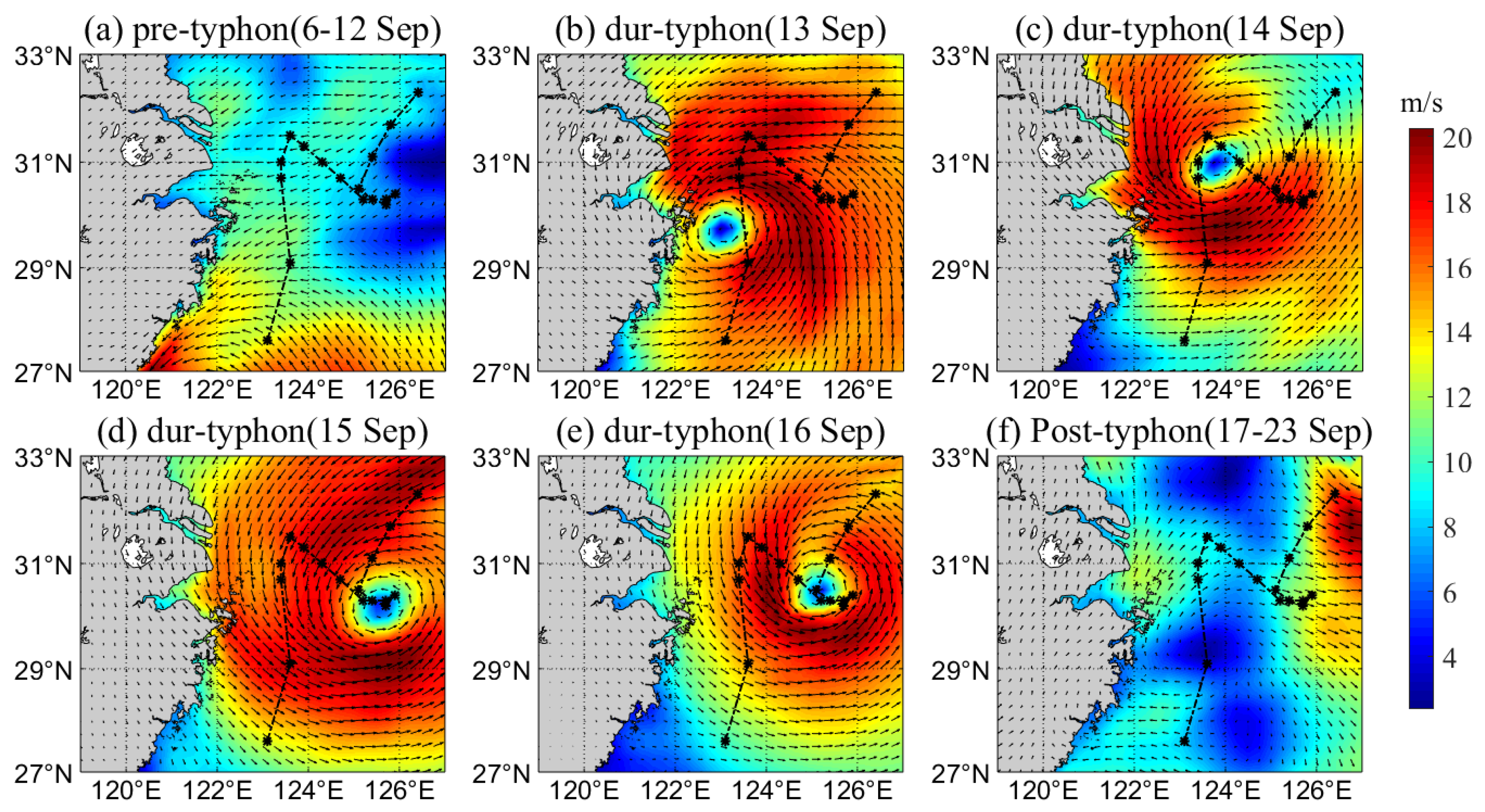
3.1. Variations in the Sea Surface Wind Field

Based on the wind speed and wind direction per hour at 10 m above the sea surface, the vector average of the wind field in the area before and after the typhoon is carried out, as shown in Figure 2. Figure 2a–f represents the wind field of the week before (6–12 September), during (13–16 September), and the week after (17–23 September), respectively. A week before the typhoon passed (Figure 2a), the wind speed was low (the mean value is 2.20 m/s), and the wind blew onshore. The south of the study area is southeast wind, the north is east wind, and the wind speed in the south is higher than in the north. During the typhoon transit period (Figure 2b–e), the wind speed increased (the mean values are 12.8 m/s, 10.9 m/s, 10.6 m/s, and 9.6 m/s, respectively), the cyclone appeared and moved from south to north along the typhoon path. The wind speed in the center of the typhoon was lower than that in the periphery of the typhoon, and the wind speed on the right side of the typhoon was higher. One week after the typhoon passed (Figure 2f), the wind speed decreased (the mean value is 1.44 m/s), the cyclone disappeared, the wind direction was irregular, and the wind speed in the west was lower than that in the east.

3.2. Distribution of SST

Based on the daily SST, the spatial distribution of SST before and after the typhoon is plotted and shown in Figure 3. Figure 3a–d represents the spatial distribution of SST in the week before (6–12 September), during (13–16 September), the week after (17–23 September), and the two weeks after (24–30 September). A week before the typhoon passed (Figure 3a), the SST was high, with an average SST of 29.01 °C. The SST in the northern part of the study area was lower than that in the south, and the SST near the coast was high, and offshore was low. During the typhoon transit period (Figure 3b), the SST in the study area decreased, with an average SST of 27.62 °C. The SST decreased from north to south, and there was a cold tongue on the left side of the typhoon path extending from north to south. One week after the typhoon passed (Figure 3c), the SST decreased, the average SST was 27.43 °C, and the cooling area appeared on the right side of the typhoon track. Two weeks after the typhoon passed (Figure 3d), the SST rose, with an average SST of 27.56 °C, lower than the SST before the typhoon passed. The spatial distribution of the SST before the typhoon passes is restored, and the north-south cold tongue disappears.

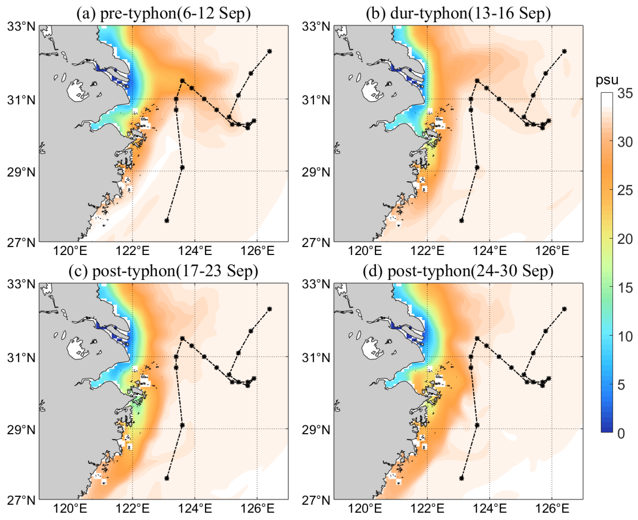
3.3. Distribution of SSS

Based on the daily SSS, the spatial distribution of the SSS before and after the typhoon is plotted and shown in Figure 4. Figure 4a–d represents the spatial distribution of SSS in the week before (6–12 September), during (13–16 September), the week after (17–23 September), and the two weeks after (24–30 September), respectively. One week before the typhoon passed (Figure 4a), the SSS was low, with an average of 30.59 psu, and the SSS gradually increased from the nearshore to the ocean. During the typhoon transit (Figure 4b), the SSS increased, with an average value of 30.87 psu. The spatial distribution of SSS is consistent with that in the early stage, but the value increased. One week after the typhoon passed (Figure 4c), the SSS decreased, averaging 30.39 psu. The spatial distribution of SSS remained unchanged, but the value decreased. Two weeks after the typhoon passed (Figure 4d), the SSS decreased, with an average SSS of 30.34 psu.

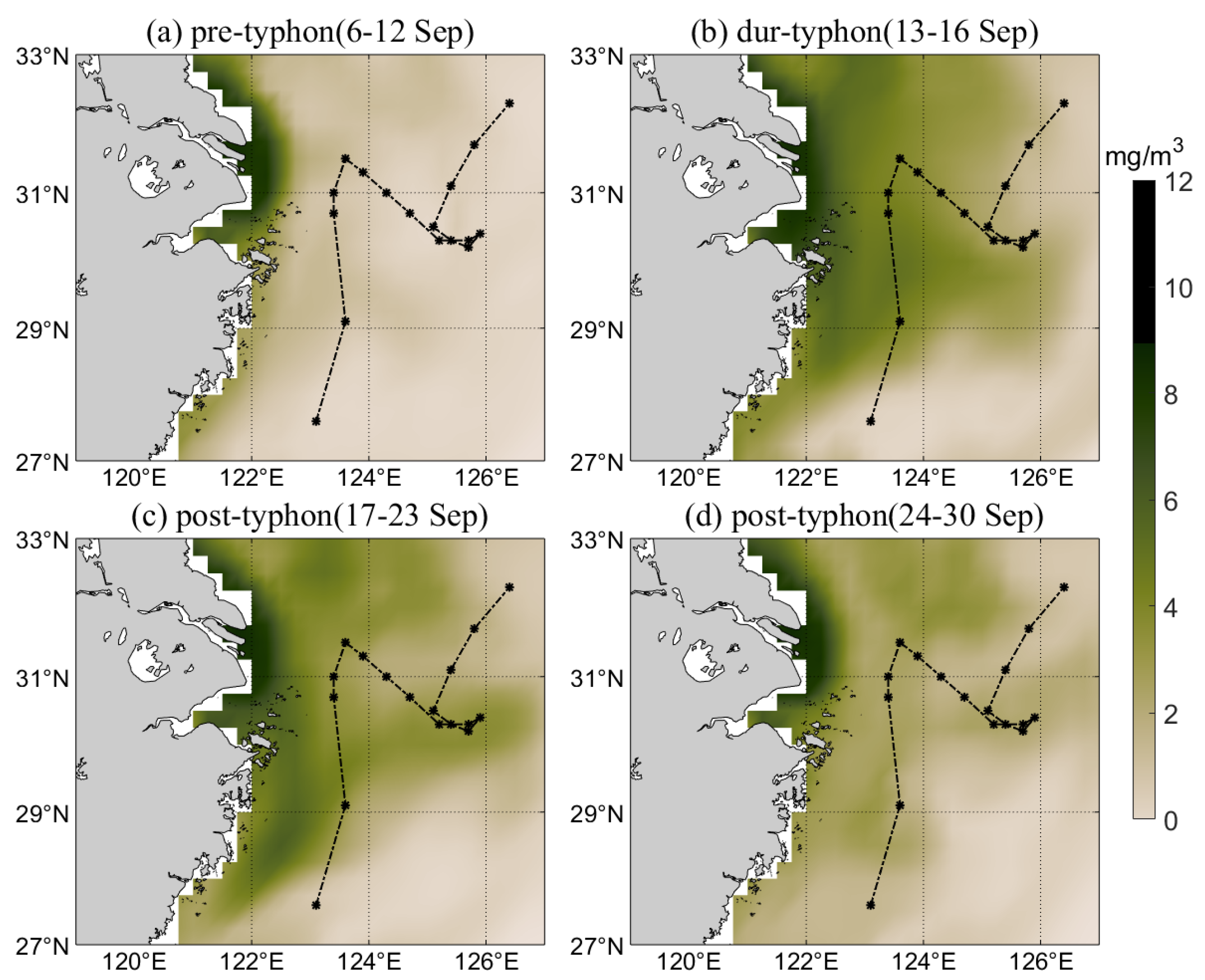
3.4. Distribution of Sea Surface Chl a

Based on the daily sea surface Chl a concentration, the spatial distribution of Chl a concentration during typhoon transit is plotted and shown in Figure 5. Figure 5a–d represents the spatial distribution of Chl a concentration in the week before (6–12 September), during (13–16 September), the week after (September 17–23), and the two weeks after (24–30 September), respectively. One week before the typhoon (Figure 5a), the concentration of Chl a was low, with an average of 0.74 mg/m3. The concentration of Chl a decreased from the coast to the ocean, and the concentration of Chl a in the Yangtze Estuary and Hangzhou Bay was the highest. During the typhoon transit period (Figure 5b), the concentration of Chl a increased, with an average value of 1.29 mg/m3, and the concentration of Chl a around the typhoon track and in the coastal waters increased significantly. One week after the typhoon passed (Figure 5c), the concentration of Chl a decreased with an average value of 1.12 mg/m3. The distribution of Chl a concentration was consistent with the previous period, but the value decreased. Two weeks after the typhoon (Figure 5d), the concentration of Chl a decreased, the average concentration of Chl a was 0.80 mg/m3, and the concentration of Chl a gradually returned to the level before the typhoon.

4. Discussion

4.1. Effect of Typhoon on EPV

To explore the influence of the typhoon on EPV, based on the hourly wind speed at 10 m above the sea surface, according to Formulas (1) and (2), the spatial distribution of EPV before and after the typhoon was obtained by calculating vector average (Figure 6). Figure 6a–f represents the spatial distribution of the EPV in the week before (6–12 September), during (13–16 September), and the week after (17–23 September), respectively. The positive value of EPV indicates an upward flow, and the negative value indicates a downward flow. One week before the typhoon passed (Figure 6a), the downdraft was dominant, and the EPV was weak, with an average rate of −6.84 × 10⁻⁶ m/s. The updraft is obvious in the south of the study area, and the downdraft was obvious in the north. During the transit period (Figure 6b–e), the updraft was dominant, and the EPV increased, with a maximum rate of 6.83 × 10⁻⁵ m/s. Along the typhoon track, a large-scale updraft area appeared on the north and south sides of the typhoon center, and a large-scale downdraft area appeared on the east and west sides. One week after the typhoon passed (Figure 6f), the study area was dominated by upwelling, and the EPV decreased, with an average rate of 6.10 × 10⁻⁷ m/s.

4.2. Effect of Typhoon on Temperature

To quantitatively analyze the variation of SST with time during typhoon transit, the SST from 1 to 12 September was the mean SST before typhoon transit. Based on this mean value, the variation of SST after wind transit (13–30 September) is analyzed (Figure 7). In Figure 7, a positive value indicates an increase in SST, and a negative value indicates a decrease. During the typhoon period, the SST indicated a downward trend as a whole. When the typhoon passed through (13th), the SST decreased, and the lowest SST decreased to 1.91 °C on the 17th. Two weeks after the typhoon, the SST rebounded; however, it still revealed a downward trend compared with the typhoon, with a decrease of 1.22 °C.
In order to analyze the spatial distribution characteristics of SST variations during typhoon transit, the SST difference between the week before typhoon transit (6–12 September) and the week after typhoon transit (17–23 September) is calculated and presented in Figure 8. The negative (positive) value indicates a decrease (increase) in SST. After the typhoon passes through, the overall SST difference in the study area is negative; that is, the SST decreases. There is a significant cooling zone on the right side of the typhoon path, and the maximum SST difference is −2.90 °C.
To analyze the impact of typhoon transit on ocean temperature, this study selected a point on the typhoon path (27.6° N, 123.1° E) to analyze the longitudinal section temperature variations based on the temperature between −85 m and 0 m before and after the typhoon transit (1–30 September) depicted in Figure 9. As shown in Figure 9, the bottom water temperature is lower than the surface water temperature. Before the typhoon passed (1–12 September), the isotherm was gentle, and the temperature of the section at one point was higher than in other periods, and the range was 19.52–29.91 °C. After the typhoon passed through (13–22 September), the isotherm rose, and the profile temperature decreased, with a range of 17.85–28.34 °C. From 23 to 30 September, the isotherm decreased, and the profile temperature increased but was still lower than before the typhoon, with a range of 17.70–28.01 °C.
Before the typhoon passed (Figure 3a), the temperature was high, the temperature difference between the north and the south was significant, and the upwelling characteristics in the coastal waters were obvious. The bottom cold water mixed with the surface water under the carrying of the upwelling [30], resulting in a low temperature in the coastal waters. Affected by the high-temperature water of the Taiwan Warm Current moving northward and the cold water moving southward along the coast, the temperature in the southeast sea area was high, and that in the northern sea area was low. During the typhoon (Figure 3c), the temperature decreased, and the water temperature decreased due to the mixing of the mixed layer and the top layer of the thermocline caused by wind stress. The largest temperature drop area was distributed on the right side of the typhoon path (Figure 8). After the typhoon (Figure 3d), the temperature rose, and the spatial distribution of temperature was consistent with that before the typhoon. Affected by the weakening of the upwelling, the temperature rose but was lower than before the typhoon.
The SST has a close response to the wind field. When Chanthu transited, due to its central low pressure and huge wind stress, it caused strong mixing and divergence in the upper ocean [31]. The typhoon deepened the mixed layer by entrainment and induced upwelling to force the redistribution of surface seawater stratification [32], resulting in a decrease in temperature.

4.3. Effect of Typhoon on Salinity

To quantitatively analyze the variation of SSS with time during typhoon transit, from 1 to 12 September, as the mean value of SSS before typhoon transit. Based on this mean value, the variation of SSS after typhoon transit (13–30 September) is analyzed (Figure 10). In Figure 10, a positive value indicates an increase in SSS, and a negative value indicates a decrease in SSS. In Figure 10, the SSS increases from 13 September to 18 and reaches the maximum on 15 September, with a difference of 0.31 psu. The SSS decreased from 19 to 30 and decreased to its lowest on 22 September, and the difference was −0.50 psu. Two weeks after the typhoon passed, the SSS rebounded, but it still illustrated a downward trend.
To analyze the spatial distribution characteristics of SSS variations during typhoon transit, the SSS difference between the week before typhoon transit (6–12 September) and the week after typhoon transit (17–23 September) is calculated (Figure 11). The negative value indicates that the SSS decreased, and the positive value indicates that the SSS increased. After the typhoon passed, the overall SSS difference in the study area was positive; that is, the SSS increased. The SSS outside the Yangtze Estuary increased significantly, with a difference of 7.75 psu. However, the SSS in the coastal waters south of Hangzhou Bay decreased significantly, with a difference of −12.00 psu.
In order to study the influence of typhoon transit on the salinity of different ocean depths, a point on the typhoon path (27.6° N, 123.1° E) was selected to analyze the salinity variations in the longitudinal section. Based on the salinity of −85 m to 0 m from before and after the typhoon transit (1–30 September), the profile variation of salinity is plotted (Figure 12). As shown in Figure 12, the bottom salinity was higher than the surface salinity. Before the typhoon passed (1–12 September), the isohaline was gentle, and the salinity of a section was low, with a range of 33.07–34.39 psu. After the typhoon passed (13–21 September), the isohaline uplifted, and the salinity at the same depth increased, with a range of 32.92–34.56 psu. From 22 to 30 September, the isohaline decreased, and the salinity at the same depth on 25 September was lower than before the typhoon, with a range of 32.85–34.58 psu.
Before the typhoon passes (Figure 4a), salinity is low, and the salinity contours expand outward parallel to the coastline. Affected by the Yangtze River’s diluted water and the high salt water of the Taiwan warm current [33], the spatial distribution of salinity was high in the southeast and low in the northwest, and the salinity in the Yangtze Estuary was the lowest. During the typhoon transit (Figure 4c), the salinity increased, and the vertical mixing caused by wind stress increased the nutrient-rich cold water in the bottom layer to the surface layer, and the salinity near the typhoon path increased. After the typhoon (Figure 4d), the salinity decreased, and the spatial distribution characteristics were consistent with those before the typhoon. Affected by the substantial increase of phytoplankton in the coastal waters, the salinity in the coastal waters decreased, which was lower than that before the typhoon, and the salinity in the adjacent waters of the Yangtze River estuary was higher than that before the typhoon.
The variation of salinity was closely related to the variation of the wind field. When Chanthu transited, strong wind stress caused a wide range of strong Ekman pumping, and the upwelling and vertical mixing were strengthened [34]. The upwelling flipped the deep cold water rich in nutrients into the upper mixed layer of the ocean through entrainment, increasing salinity [35].

4.4. Effect of Typhoon on Chl a Concentration

To quantitatively analyze the variation of Chl a concentration over time during typhoon transit, the sea surface Chl a concentration from 1 to 12 September was the mean value of sea surface Chl a concentration before the typhoon. Based on this mean value, the variation of sea surface Chl a concentration after the typhoon transited (13–30 September) was analyzed (Figure 13). In Figure 13, a positive value indicates an increase in Chl concentration, and a negative value indicates a decrease. The concentration of Chl a on the sea surface increased after the typhoon and reached the highest value of 0.86 mg/m3 on the 17th. After 17 days, the concentration of Chl a on the sea surface decreased slowly, but it was still higher than before the typhoon. Two weeks after the typhoon (30 September) passed, the concentration of Chl a returned to pre-typhoon levels.
In order to analyze the spatial distribution of sea surface Chl a concentration variations during typhoon transit, based on the mean value of Chl a concentration in the week before typhoon transit (6–12 September), the variation of sea surface Chl a concentration in the week after typhoon transit (17–23 September) was analyzed, as shown in Figure 14. In Figure 14, the negative value indicates the decrease of Chl a concentration, and the positive value indicates the increase. After the typhoon passed, the difference in Chl a concentration in the study area was positive (that is, the Chl a concentration increases). Chl a concentration in the coastal waters and the right side of the typhoon path increased significantly, and the maximum difference was 2.63 mg/m3.
In order to study the effect of typhoon transit on Chl a concentration in different depth profiles, a point on the typhoon path (27.6° N, 123.1° E) was selected to analyze the variation of Chl a concentration in the longitudinal section. Based on the Chl a concentration of −90 m to 0 m from the sea surface depth before and after the typhoon (1–30 September), the profile variation of Chl a concentration was drawn (Figure 15). From Figure 15, it can be seen that the area with high Chl a concentration was located in the middle layer, and the Chl a concentration in the surface and bottom layers was low. The Chl a concentration illustrates a ‘Subsurface Chla maximum‘ variation from the bottom layer to the sea surface. After the typhoon passed through, the high-value area of Chl a concentration increased compared with that before. Before the typhoon (1–12 September), the concentration of Chl a in the profile was the lowest, and the range was 0.12–1.23 mg/m3. The value was the highest 10 days after the typhoon (25 September), the range was 0.09–2.94 mg/m3, and the concentration of Chl a in other periods was in the middle.
Before the typhoon (Figure 5a), the concentration of Chl a was low. Due to the eutrophication caused by the large amount of nutrients carried by the Yangtze River diluted water, the concentration of Chl a indicated the spatial distribution characteristics of high near shore and low offshore, and the concentration of Chl a in the Yangtze River Estuary was the highest. During the typhoon transit period (Figure 5b), the concentration of Chl a increased. Affected by the upwelling caused by the typhoon, the cold water rich in nutrients in the deep layer was transported to the surface of the ocean, creating favorable conditions for the reproduction and growth of phytoplankton. After the typhoon passed (Figure 5d), the concentration of Chl a decreased, and the spatial distribution characteristics of Chl a concentration on the sea surface were consistent with those before the typhoon. The vertical mixing of water bodies weakened, the concentration of nutrients on the sea surface decreased, and the concentration of Chl a decreased. Two weeks after the typhoon (30 September) passed, the concentration of Chl a returned to the pre-typhoon level.
To better analyze the source of the increase in Chl a concentration at the sea surface during the typhoon transit, Chl a concentration at depths of 20 m, 40 m, and 80 m in the study sea area was selected to analyze the concentration changes. As shown in Figure 16, the highest Chl a concentration was found at 20 m, with a mean value of 0.805 mg/m3; the lowest Chl a concentration was found at 80 m, with a mean value of 0.301 mg/m3; and the second highest was found at 40 m, with a mean value of 0.661 mg/m3. During the typhoon’s passage, the concentration of Chl a varied considerably at 20 m and 40 m, and the concentration of Chl a generally increased for 5 days after the typhoon’s passage (18th day). The Chl a concentration at 80 m showed a small change, and after the 13th day, the Chl a concentration generally showed an increasing trend. Therefore, the main source of the increase in Chl a concentration at the surface during the typhoon’s transit was not due to upwelling carrying bottom Chl a to the surface.
The rapid increase of Chl a concentration in the short term was related to the variation of the wind field in the same period. The strong wind event caused by Chanthu caused strong disturbance and water surge in the upper layer of the ocean in the shallow waters of the nutrient layer, so that the oligotrophic and euphotic layer in the upper layer was supplemented by a large amount of nutrients [36,37,38,39,40]. The heavy precipitation caused by Chandu transported nutrients from the coastal waters to the sea, resulting in the rapid reproduction of phytoplankton in the typhoon path and the southern coastal waters.

5. Conclusions

In this paper, the variations of temperature, salinity, and Chl a concentration in some sea areas affected by typhoon Chanthu are analyzed by remote sensing reanalysis data before and after the passage of typhoon Chanthu, and the modification mechanism is studied. The conclusions are as follows:
(1)
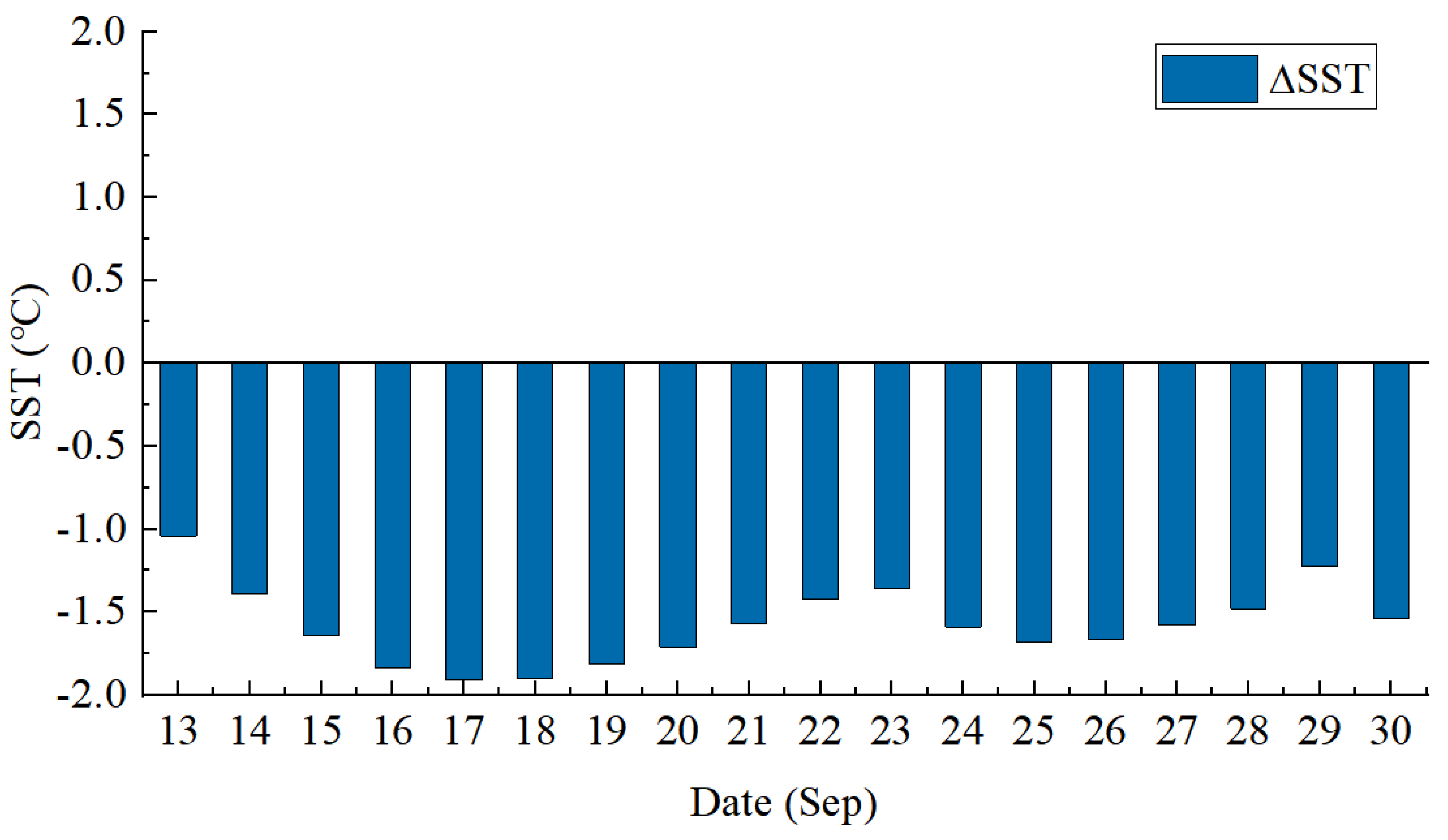
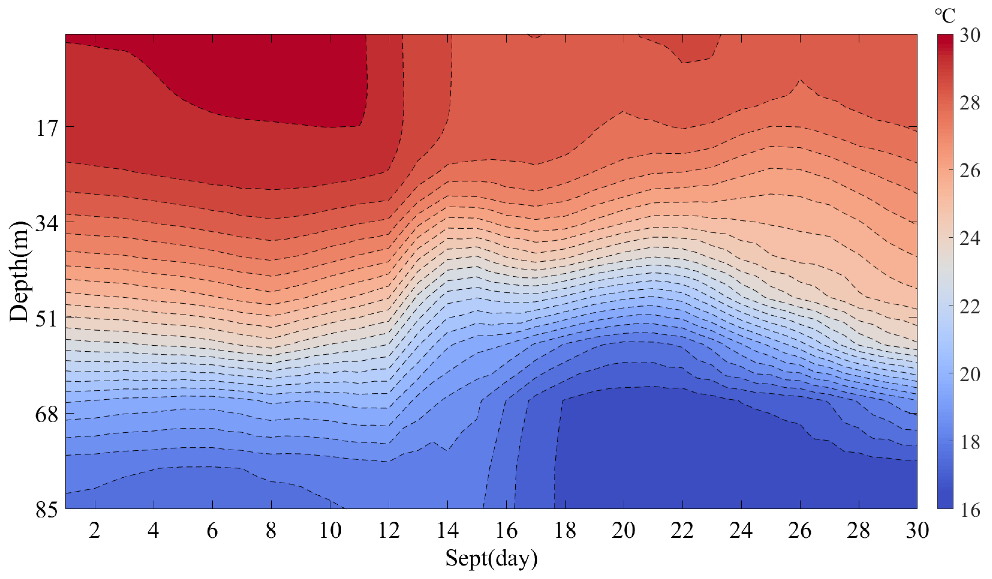
The transit of Chanthu reduced the SST by an average of 1.58 °C, and the cooling process lasted more than two weeks. The SST on the right side of the typhoon track decreased significantly, and the cooling was right-skewed. The SST rebounded two weeks after the typhoon, but it was still lower than before. The SST drop was mainly affected by the deep cold water upwelling and seawater mixing caused by the typhoon;
(2)
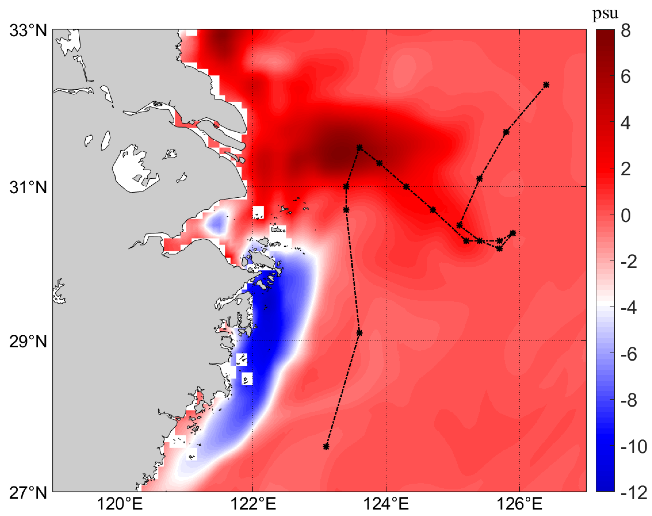
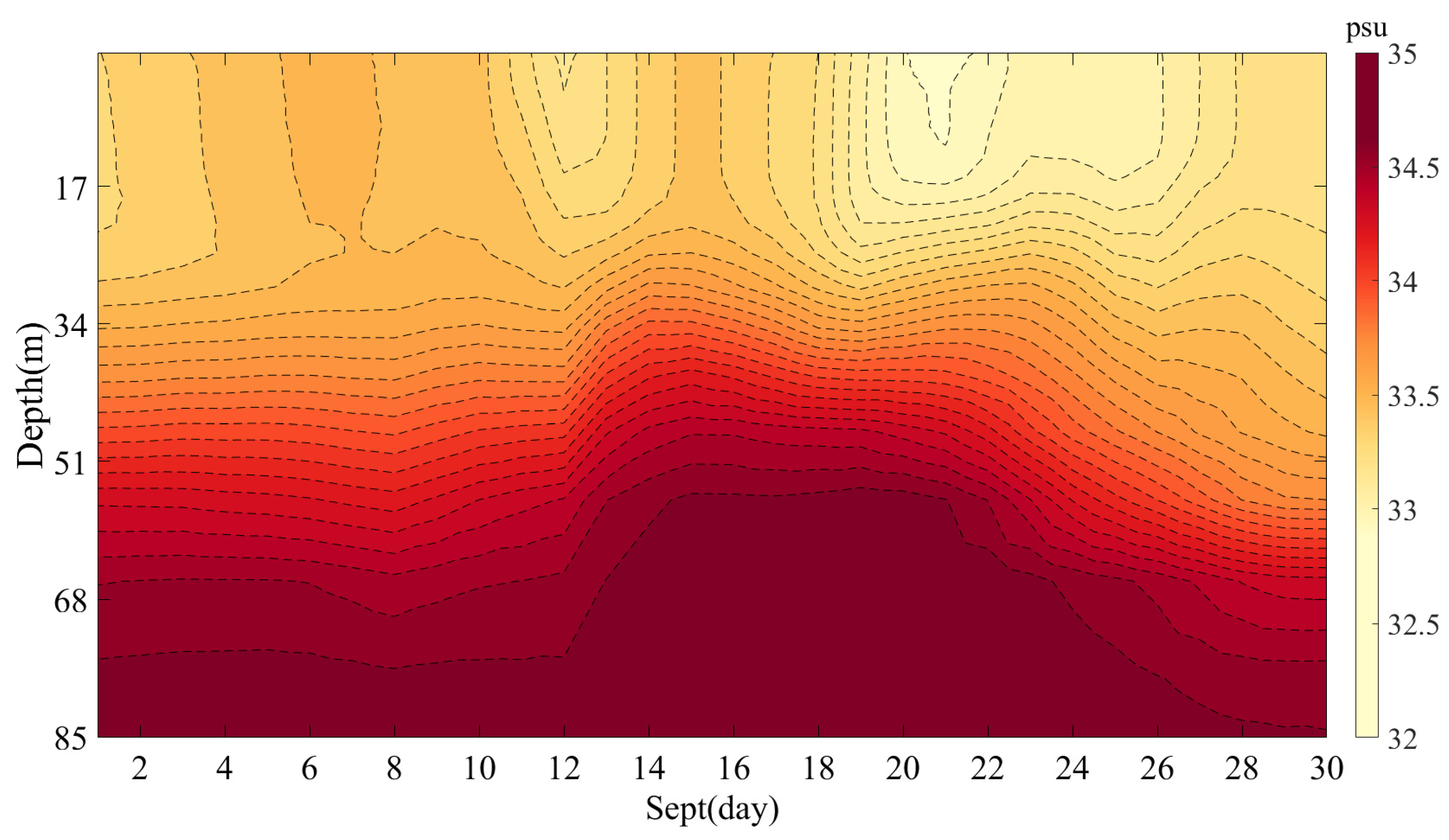
The SSS of the sea area affected by Canhtu increased by an average of 0.28 psu. The SSS growth continued for six days and reached its highest on the third day. The SSS decreased one week after transit and decreased to the lowest on the 10th day. The whole decline process lasted for two weeks. The SSS rising area was mainly concentrated in the coastal waters of the Yangtze River estuary, and the falling area was mainly distributed in the south of Hangzhou Bay. The increased SSS was mainly affected by the upwelling of deep, high salt water. The decreased SSS was mainly affected by the weakening and disappearance of upwelling caused by the departure of the typhoon and the rainfall caused by the typhoon;
(3)
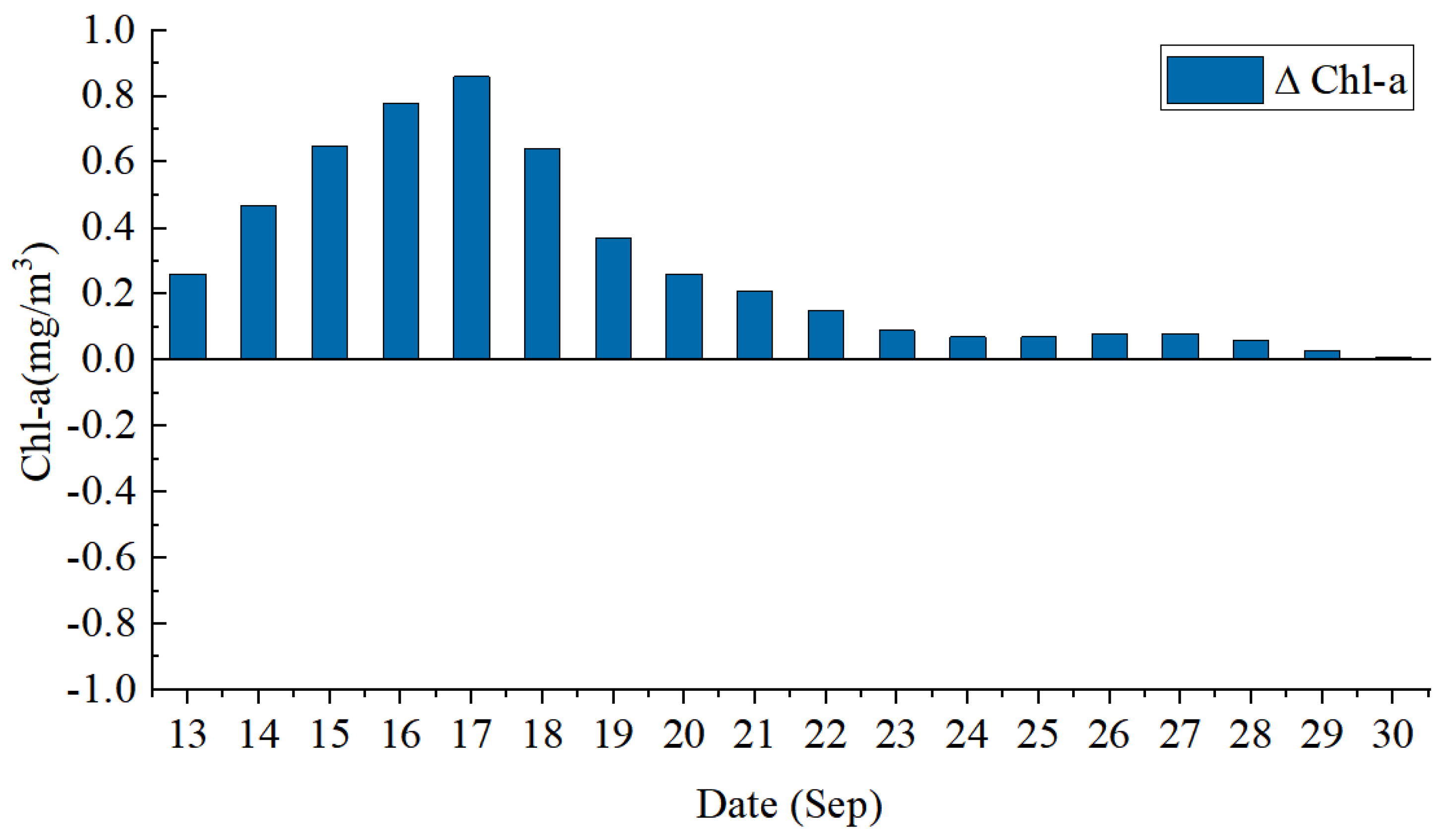
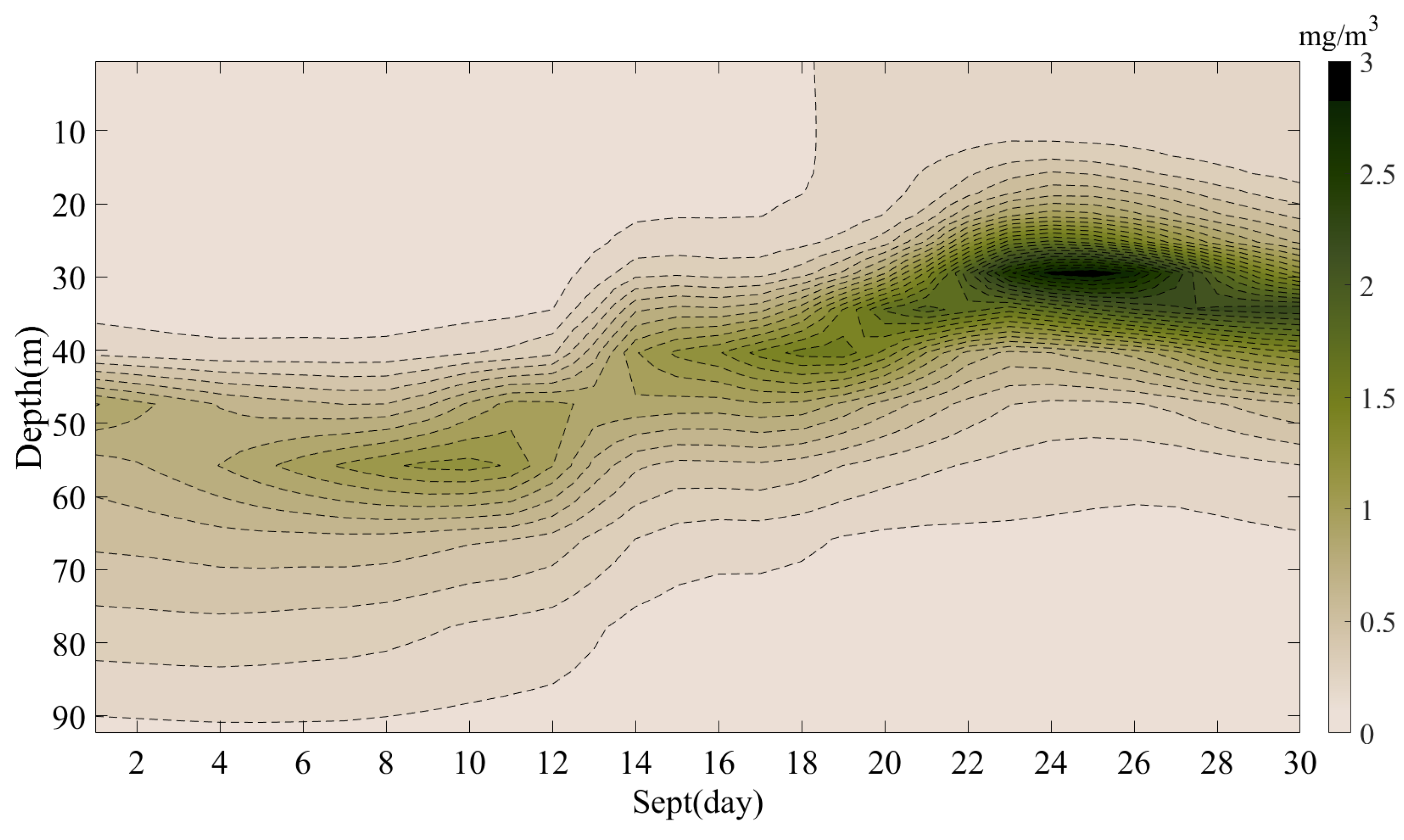
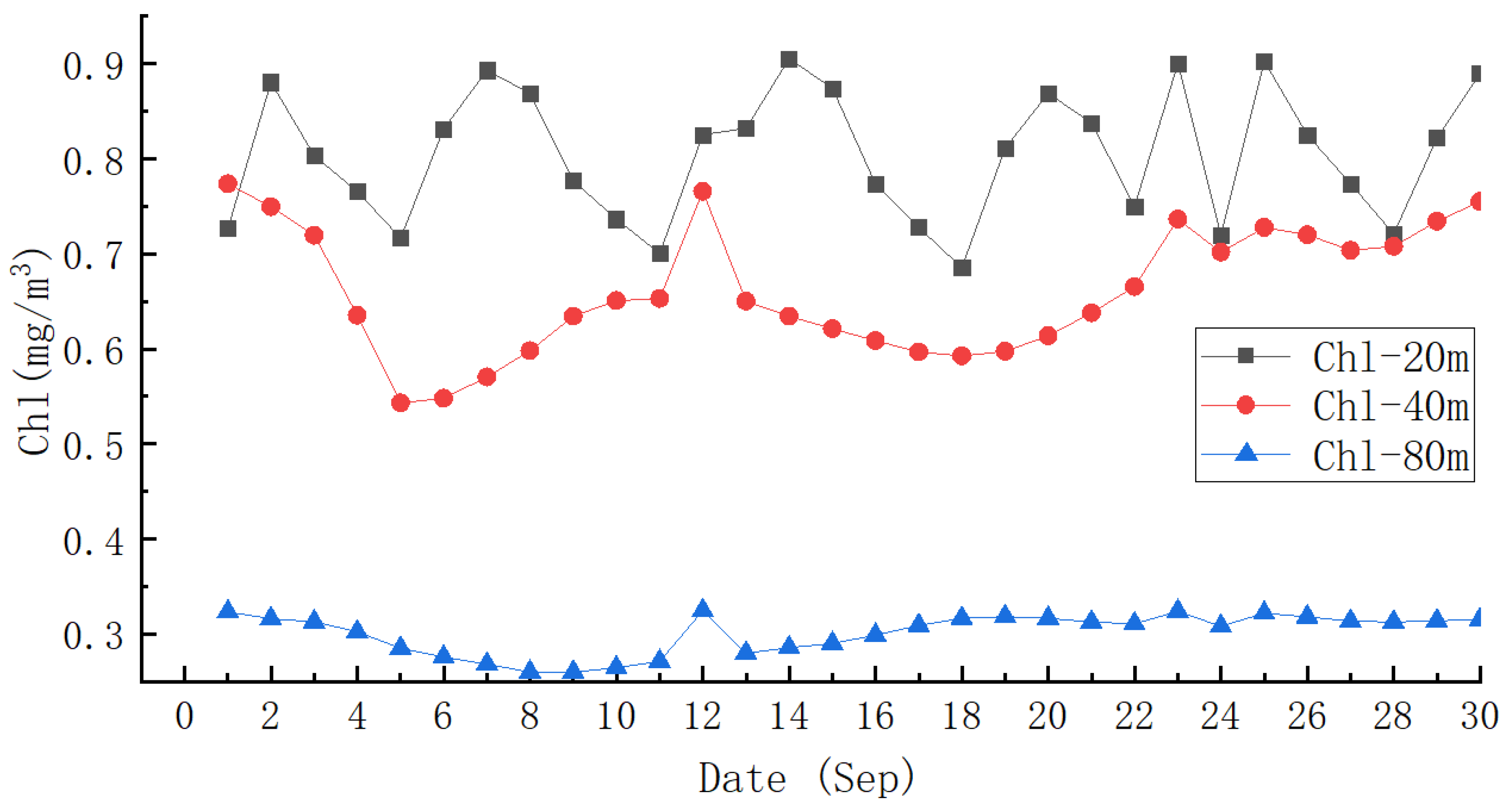
The influence of Chanthu increased the concentration of Chl a in the study area to 0.74 times higher than before. The whole growth process lasted for two weeks, and the maximum value appeared on the fifth day after the typhoon. The response of Chl a to the typhoon had a certain delay, and the increased area was mainly concentrated near the typhoon path and offshore waters. The increase of Chl a concentration was mainly affected by the strengthening of marine dynamic mechanisms, such as seawater mixing and upwelling caused by the typhoon and the influence of continental runoff.
Chl a concentration is an important indicator of the amount of marine photoautotrophic organisms and plays an important role in the material cycle and energy conversion process of marine ecology. The results of this paper are of great significance for the study of the carbon cycle, environmental monitoring, red tide disaster monitoring, ocean current (upwelling, coastal current), and fishery management in the ocean-atmosphere system.

Author Contributions

Conceptualization, J.W., B.G., Y.C. and Z.J.; methodology, J.W.; software, J.W.; validation, J.W., B.G. and V.S.M.; formal analysis, J.W.; investigation, J.W.; resources, B.G.; data curation, J.W.; writing—original draft preparation, J.W.; writing—review and editing, B.G. and V.S.M.; visualization, J.W.; supervision, B.G.; project administration, B.G.; funding acquisition, B.G. All authors have read and agreed to the published version of the manuscript.

Funding

This work was mainly supported by the open research fund program of State Key Laboratory of Hydroscience and Engineering, Tsinghua University (sklhse-2021-B-01); Consultation and Evaluation Program of the Department of Chinese Academy of Science (2020-ZW11-A-023); the National Natural Science Foundation of China (Grant No. 51979264 and 51479179); and Zhejiang Provincial Virtual Simulation Experiment Projects (virtual simulation experiment project of monitoring of suspended sediment in coastal waters using remote sensing).

Institutional Review Board Statement

Not applicable.

Informed Consent Statement

Not applicable.

Data Availability Statement

Not applicable.

Conflicts of Interest

The authors declare no conflict of interest.

References

  1. Falkowski, P.G. The role of phytoplankton photosynthesis in global biogeochemical cycles. Photosynth Res. 1994, 39, 235–258. [Google Scholar] [CrossRef] [PubMed]
  2. Zhao, H.; Wang, Y. Phytoplankton Increases Induced by Tropical Cyclones in the South China Sea During 1998–2015. J. Geophys. Res. Ocean. 2018, 123, 2903–2920. [Google Scholar] [CrossRef]
  3. Hallegraeff, G.M. A review of harmful algal blooms and their apparent global increase. Phycologia 1993, 32, 79–99. [Google Scholar] [CrossRef]
  4. Price, J.F. Upper ocean response to a hurricane. J. Phys. Oceanogr. 1981, 11, 153–175. [Google Scholar] [CrossRef]
  5. Font, J.; Kerr, Y.H.; Srokosz, M.A.; Etcheto, J.; Lagerloef, G.S.; Camps, A.; Waldteufel, P. SMOS: A Satellite Mission to Measure Ocean Surface Salinity. Conf. Atmos. Propag. Adapt. Syst. Laser Radar Technol. Remote Sens. 2001, 4167, 207–214. [Google Scholar]
  6. Yin, X.B. A Study on the Passive Microwave Remote Sensing of Sea Surface Wind Vector, Temperature and Salinity and the Effect of Wind on Remote Sensing of Temperature and Salinity; Ocean University of China: Qingdao, China, 2007. [Google Scholar]
  7. Cao, K.X.; Jin, X.F.; Sun, W.F.; Wang, J. Quality assessment and correction of SST fusion product in the Bohai Sea and the Huanghai Seas. Mar. Sci. 2017, 41, 50–55. [Google Scholar]
  8. Mecklenburg, S.; Drusch, M.; Kerr, Y.H.; Font, J.; Martin-Neira, M.; Delwart, S.; Buenadicha, G.; Reul, N.; Daganzo-Eusebio, E.; Oliva, R.; et al. ESA’s Soil Moisture and Ocean Salinity Mission: Mission Performance and Operations. IEEE Trans. Geosci. Remote Sens. 2012, 50, 1354–1366. [Google Scholar] [CrossRef]
  9. Stramma, L.; Cornillon, P.; Price, J.F. Satellite observations of sea surface cooling by hurricanes. J. Geophys. Res. Ocean. 1986, 91, 5031–5035. [Google Scholar] [CrossRef]
  10. Zhao, H.; Tang, D.L.; Wang, Y. Comparison of phytoplankton blooms triggered by two typhoons with different intensities and translation speeds in the South China Sea. Mar. Ecol. Prog. Ser. 2008, 365, 57–65. [Google Scholar] [CrossRef]
  11. Shi, W.; Wang, M. Observations of a hurricane katrina-induced phytoplankton bloom in the gulf of Mexico. Geophys. Res. Lett. 2007, 34, 607–612. [Google Scholar] [CrossRef]
  12. Lin, I.I.; Liu, W.T.; Wu, C.C.; Chiang, J.C.; Sui, C.H. satellite observations of modulation of surface winds by typhoon-induced upper ocean cooling. Geophys. Res. Lett. 2003, 30, 1-131–1-135. [Google Scholar] [CrossRef]
  13. Lin, I.; Liu, W.T.; Wu, C.C.; Wong, G.T.; Hu, C.; Chen, Z.; Liang, W.D.; Yang, Y.; Liu, K.K. New evidence for enhanced ocean primary production triggered by tropical cyclone. Geophys. Res. Lett. 2003, 30, 1718–1722. [Google Scholar] [CrossRef]
  14. Walker, N.D.; Leben, R.R.; Balasubramanian, S. Hurricane-forced upwelling and chlorophyll a enhancement within cold-core cyclones in the Gulf of Mexico. Geophys. Res. Lett. 2005, 32, L18610. [Google Scholar] [CrossRef]
  15. Narvekar, J.; Roy Chowdhury, R.; Gaonkar, D.; Kumar, P.D.; Prasanna Kumar, S. Observational evidence of stratification control of upwelling and pelagic fishery in the eastern Arabian Sea. Sci. Rep. 2021, 11, 7293. [Google Scholar] [CrossRef] [PubMed]
  16. Yin, X.; Wang, Z.; Liu, Y.; Xu, Y. Ocean response to Typhoon Ketsana traveling over the northwest Pacific and a numerical model approach. Geophys. Res. Lett. 2007, 34, L21606-1–L21606-6. [Google Scholar] [CrossRef]
  17. Cao, K.X.; Sun, W.F.; Meng, J.M.; Zhang, J. Assessment and Comparison of Sea Surface Salinity Data Derived From SMAP and SMOS Based on Argo M easurements. Adv. Mar. Sci. 2019, 37, 574–587. [Google Scholar]
  18. Bhaskar, T.V.S.U.; Jayaram, C. Evaluation of Aquarius Sea Surface Salinity with Argo Sea Surface Salinity in the Tropical Indian Ocean. Geosci. Remote Sens. Lett. IEEE 2015, 12, 1292–1296. [Google Scholar] [CrossRef]
  19. Tang, W.; Yueh, S.H.; Fore, A.G.; Hayashi, A. Validation of Aquarius sea surface salinity with in situ measurements from Argo floats and moored buoys. J. Geophys. Res. Ocean. 2014, 119, 6171–6189. [Google Scholar] [CrossRef]
  20. Le Vine, D.M.; Lagerloef, G.S.E.; Torrusio, S.E. Aquarius and Remote Sensing of Sea Surface Salinity from Space. Proc. IEEE 2010, 98, 688–703. [Google Scholar] [CrossRef]
  21. Just! Typhoon Chando, the 14th Typhoon of This Year, Formed in the Northwest Pacific Ocean. China Weather Network, 2021. Available online: http://news.weather.com.cn/2021/09/3491355.shtml (accessed on 21 July 2023).
  22. Typhoon ‘Chandu’ Was Generated and Is Expected to Affect the Offshore Fishing Grounds in Fujian after 11 Days. Guangzhou Daily. 2021. Available online: https://www.gzdaily.cn/amucsite/web/index.html#/detail/1653936 (accessed on 21 July 2023).
  23. Typhoon Chanthu No. 14 Strengthened into a Super Typhoon, and will Be Seen Tomorrow or Near the Coast of Guangdong and Fujian. Guangzhou Daily. 2021. Available online: https://baijiahao.baidu.com/s?id=1710293479196671127&wfr=spider&for=pc (accessed on 21 July 2023).
  24. This year’s No.14 Typhoon Canyon landed in Fukuoka County, Japan Only. CCTV News. 2021. Available online: http://m.news.cctv.com/2021/09/17/ARTIrjf44FLbHGzDC7al7EIJ210917.shtml (accessed on 21 July 2023).
  25. Monod, J. Recherches sur la Croissance des Cultures Bactériennes; Hermann: Paris, France, 1942; p. 1377. [Google Scholar]
  26. Geider, R.J.; Macintyre, H.L.; Kana, T.M. A dynamic model of photoadaptation in phytoplankton. Limnol. Oceanogr. 1996, 41, 1–15. [Google Scholar] [CrossRef]
  27. Geider, R.J.; Macintyre, H.L.; Kana, T.M. Dynamic model of phytoplankton growth and acclimation: Responses of the balanced growth rate and the chlorophyll a:carbon ratio to light, nutrient-limitation and temperature. Mar. Ecol. Prog. 1997, 148, 187–200. [Google Scholar] [CrossRef]
  28. Ch, V.; Deo, A.A. Study of upper ocean parameters during passage of tropical cyclones over Indian seas. Int. J. Remote Sens. 2019, 40, 4683–4723. [Google Scholar] [CrossRef]
  29. Taylor, G.I. Skin Friction of the Wind on the Earth’s Surface. Proceedings of the Royal Society of London. Ser. A Contain. Pap. A Math. Phys. Character 1916, 92, 196–199. [Google Scholar]
  30. Hu, M.G.; Zhao, C.F. Upwelling in Zhejang Coastal Areas during Suummer Detected by Satellite observations. Natl. Remote Sens. Bull. 2008, 12, 297–304. [Google Scholar]
  31. Liu, Z.H.; Xu, J.P.; Zhu, B.K.; Sun, Z.; Zhang, L. Upper ocean response to tropical cyclones in northwestern Pacific during 2001–2004 by Argo data. J. Trop. Ocean. 2006, 25, 1–8. [Google Scholar]
  32. Chang, Y.; Liao, H.-T.; Lee, M.-A.; Chan, J.-W.; Shieh, W.-J.; Lee, K.-T.; Wang, G.-H.; Lan, Y.-C. Multisatellite observation on upwelling after the passage of Typhoon Hai-Tang in the southern East China Sea. Geophys. Res. Lett. 2008, 35, 3612-1–3612-5. [Google Scholar] [CrossRef]
  33. Beardsley, R.; Limeburner, R.; Yu, H.; Cannon, G. Discharge of the Changjiang (Yangtze River) into the East China Sea. Cont. Shelf Res. 1985, 4, 57–76. [Google Scholar] [CrossRef]
  34. Lin, I.-I.; Wu, C.-C.; Pun, I.-F.; Ko, D.-S. Upper-ocean thermal structure and the western North Pacific category 5 typhoons. Part I: Ocean features and the category 5 typhoons’ intensification. Mon. Weather Rev. 2008, 136, 3288–3306. [Google Scholar] [CrossRef]
  35. Shang, S.; Li, L.; Sun, F.; Wu, J.; Hu, C.; Chen, D.; Ning, X.; Qiu, Y.; Zhang, C.; Shang, S. Changes of temperature and bio-optical properties in the South China Sea in response to Typhoon Lingling, 2001. Geophys. Res. Lett. 2008, 35, L10602-1–L10602-6. [Google Scholar] [CrossRef]
  36. McKinnon, A.D.; Meekan, M.G.; Carleton, J.H.; Furnas, M.; Duggan, S.; Skirving, W. Rapid changes in shelf waters and pelagic communities on the southern Northwest Shelf, Australia, following a tropical cyclone. Cont. Shelf Res. 2003, 23, 93–111. [Google Scholar] [CrossRef]
  37. Shiah, F.-K.; Chung, S.-W.; Kao, S.-J.; Gong, G.-C.; Liu, K.-K. Biological and hydrographical responses to tropical cyclones(typhoons) in the continental shelf of the Taiwan Strait. Cont. Shelf Res. 2000, 20, 2029–2044. [Google Scholar] [CrossRef]
  38. Zhao, H.; Tang, D.L.; Wang, D.X. Phytoplankton blooms near the Pearl River estuary induced by Typhoon Nuri. J. Geophys. Res. Ocean. 2009, 114, 1–9. [Google Scholar] [CrossRef]
  39. Fu, D.Y.; Pan, D.L.; Ding, Y.Z.; Zou, J.H. Quantitative study of effects of the sea chlorophyl-a concent ration by typhoon based on remote sensing. Haiyang Xuebao 2009, 31, 46–56. [Google Scholar]
  40. Fu, D.Y.; Ding, Y.Z.; Liu, D.Z.; Pan, D.L. Remote- Sensing Study of the Effect of Typhoon on Chlorophyll-a Concentration in the Southeast China Sea. J. Guangdong Ocean Univ. 2008, 28, 73–76. [Google Scholar]
Figure 1. Path of typhoon Chanthu. The left image illustrates the typhoon track (7–18 September), and the right image illustrates the study area (119–127° E, 27–33° N). Atmosphere 14 01505 i001 represents the tropical depression, Atmosphere 14 01505 i002 represents the tropical storm, Atmosphere 14 01505 i003 represents the strong tropical storm, Atmosphere 14 01505 i004 represents the typhoon, Atmosphere 14 01505 i005 represents the strong typhoon, Atmosphere 14 01505 i006 represents the super typhoon, and the circular size represents the typhoon intensity.
Atmosphere 14 01505 g001
Figure 2. Spatial distribution of wind field (wind speed (m/s), wind direction) during typhoon transit. (af) represent the spatial distribution of the sea surface wind field in the week before the typhoon (6–12 September), during the period (13–16 September), and the week after the typhoon (17–23 September). The direction of the black arrow indicates the wind direction, and the color from blue to red indicates that the wind speed gradually increases. The black dotted line indicates the typhoon path, and the black dot indicates the typhoon center.
Atmosphere 14 01505 g002
Figure 3. Spatial distribution of SST (°C) during typhoon transit. (ad) represent the spatial distribution of SST in the week before (6–12 September), during (13–16 September), the week after (17–23 September) and the two weeks after (24–30 September). The black dotted line indicates the typhoon path, and the black dot indicates the typhoon center.
Atmosphere 14 01505 g003
Figure 4. Spatial distribution of SSS (psu) during typhoon transit. (ad) represent the spatial distribution of SSS in the week before (6–12 September), during (13–16 September), the week after (17–23 September) and the two weeks after (24–30 September). The black dotted line indicates the typhoon path, and the black dot indicates the typhoon center.
Atmosphere 14 01505 g004
Figure 5. Spatial distribution of sea surface Chl a concentration during typhoon transit. (ad) represent the spatial distribution of Chl a concentration in the week before (6–12 September), during (13–16 September), the week after (17–23 September), and the two weeks after (24–30 September). The black dotted line indicates the typhoon path, and the black dot indicates the typhoon center.
Atmosphere 14 01505 g005
Figure 6. Spatial variation of EPV (m/s) during typhoon transit. (af) represent the spatial distribution of EPV in the week before typhoon transit (6–12 September), during typhoon transit (13–16 September), and the week after typhoon transit (17–23 September), respectively. The black dotted line indicates the typhoon path, and the black dot indicates the typhoon center.
Atmosphere 14 01505 g006
Figure 7. Variations in SST during typhoon transit compared with the mean value (13–30 September). The abscissa represents the time (13–30 September), and the ordinate represents the SST variation.
Atmosphere 14 01505 g007
Figure 8. Spatial distribution of SST difference before and after typhoon transit.
Atmosphere 14 01505 g008
Figure 9. Temperature profile at a point (27.6° N, 123.1° E) on the track during typhoon transit. The abscissa represents the date (1–30 September), the ordinate represents the seawater depth (−851–300 m), the dotted line represents the isotherm, and the color from blue to red indicates that the temperature gradually increases.
Atmosphere 14 01505 g009
Figure 10. Variations in SSS during typhoon transit compared with the mean value (13–30 September). The abscissa represents the date (13–30 September), and the ordinate represents the SSS variation.
Atmosphere 14 01505 g010
Figure 11. Spatial distribution of SSS difference during typhoon transit. The abscissa represents the date, and the ordinate represents the depth. The color from blue to red indicates an increase in SSS.
Atmosphere 14 01505 g011
Figure 12. Salinity profile at a point (29.1° N–123.6° E) on the track during typhoon transit. The abscissa represents the time (1–3 September), the ordinate represents the depth of seawater (−85–0 m), the dotted line represents the isotherm, and the color from yellow to red indicates that the salinity increases gradually.
Atmosphere 14 01505 g012
Figure 13. Variations of sea surface Chl a concentration during typhoon transit compared with the mean value (13–30 September). The abscissa represents the date (13–30 September), and the ordinate represents the difference in Chl a concentration (mg/m3).
Atmosphere 14 01505 g013
Figure 14. Spatial distribution of Chl a concentration difference during typhoon transit.
Atmosphere 14 01505 g014
Figure 15. Chl a concentration profile at a point (27.6° N, 123.1° E) on the track during typhoon transit. The abscissa represents the time (1–30 September), the ordinate represents the depth of seawater (−90–0 m), the dotted line represents the isoline of Chl a concentration, and the color from light green to dark green indicates an increase in Chl a concentration.
Atmosphere 14 01505 g015
Figure 16. Variation of chlorophyll a concentration at different depths (20 m, 40 m, 80 m) during typhoon transit.
Atmosphere 14 01505 g016
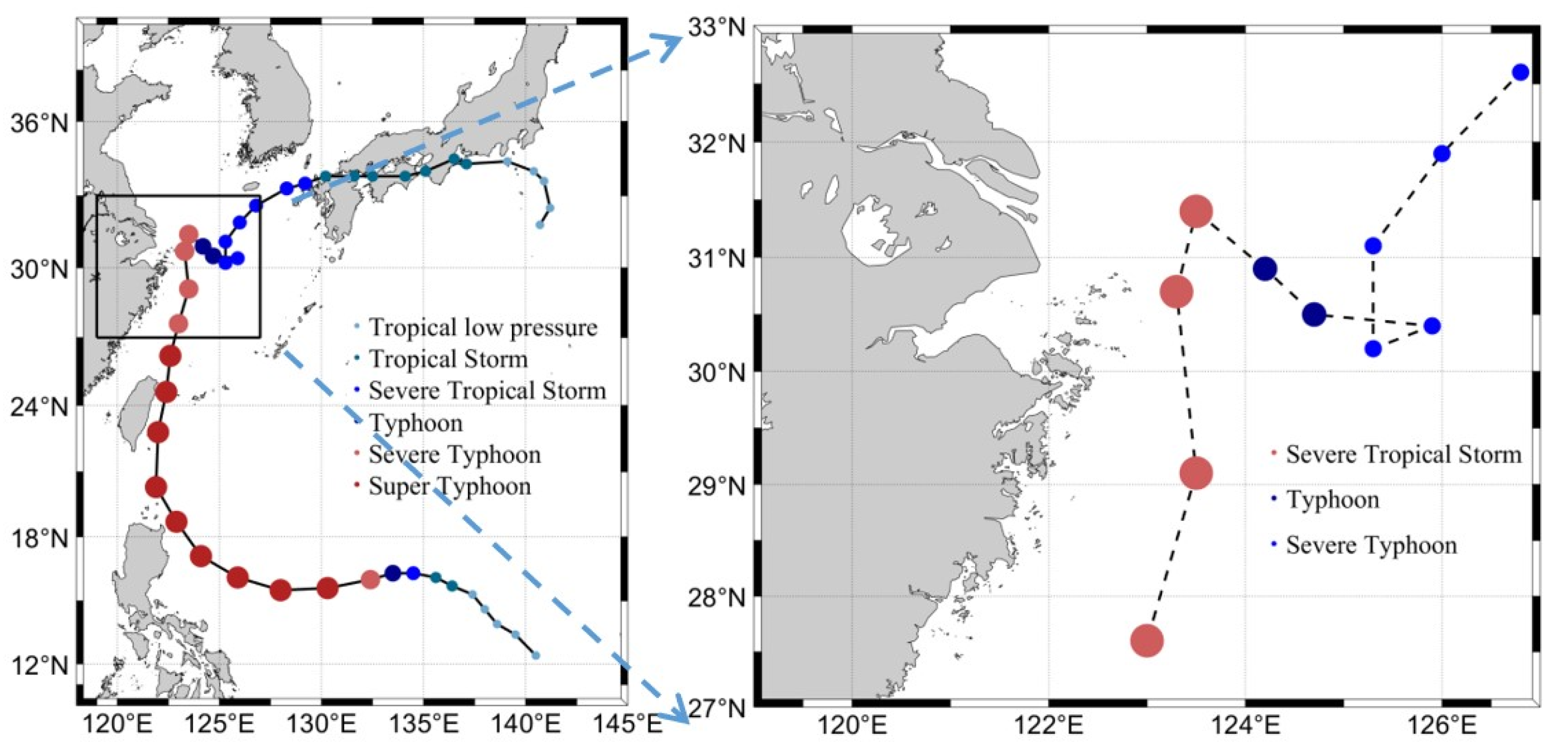
Disclaimer/Publisher’s Note: The statements, opinions and data contained in all publications are solely those of the individual author(s) and contributor(s) and not of MDPI and/or the editor(s). MDPI and/or the editor(s) disclaim responsibility for any injury to people or property resulting from any ideas, methods, instructions or products referred to in the content.

