Spatial Effects of Urban Transport on Air Pollution in Metropolitan Municipalities of Mexico

Abstract

The objective of this work was to estimate the local effects and spatial spillover effects of the number of vehicles, use of urban public transport, and population density on nitrogen oxide emissions for 405 metropolitan municipalities in Mexico in 2016. To this end, a Spatial Durbin Model was estimated. We found positive direct effects of the number of vehicles and population density and negative direct effects of the use of urban public transport. The number of vehicles in circulation had negative spillover effects on the nitrogen oxide emissions of neighboring municipalities. These results indicate that the design of public policy programs aimed at reducing air pollution in Mexico should be based on coordination across metropolitan municipalities.

1. Introduction

Factors such as economic growth, industrialization, transport of goods, energy intensity, structure of electric power generation, environmental regulation, land urbanization, and urban structure, as well as traffic intensity and mobility patterns, are the main drivers of pollutant gas emissions from fixed and mobile sources on a global and local scale. Knowing the spatial scope of their impacts is required to measure their effects on ecosystems and population health. Most of the literature on pollutant gas emissions has focused on the main sources and drivers, material composition, physicochemical reactions in the atmosphere, environmental pollution, and damage to human health. The environmental impact of these gases on the atmosphere can be classified by their global and local effects. According to Lehmann [1], and Baiardi [2], global pollutant emissions are those with marginal damage that does not depend on the location of the emission and reception. Local emissions are those for which any marginal damage depends on the location of the emission and reception. The main pollutant emissions causing global climate change include carbon dioxide $\left(C{O}_2\right)$, methane $\left(C{H}_4\right)$, and nitrous oxides $\left(N_{2}O\right)$. Local pollutant emissions include volatile organic compounds $\left(COVs\right)$, nitrogen oxides $\left(NOx\right)$, and sulfur dioxide $\left(S{O}_2\right)$ [2]. Nitrogen Oxides $\left(NOx\right)$ are a group of gases composed of Nitric Oxide ($NO$) and Nitrogen Dioxide ($N{O}_2$), this characterized for being a toxic gas. Most anthropogenic emissions of nitrogen oxides have, as their common origin, the combustion of fossil fuels, which causes air pollution problems in large urban areas with high levels of vehicular traffic. This is because nitrogen oxides ($NOx$) together with non-methane volatile organic compounds ($NMVOC$) and carbon monoxide ($CO$) constitute the main precursors of tropospheric ozone ($O_3$), since $O_3$ is a secondary pollutant from the photochemical reaction of $NMVOC$ and $NOx$ [3,4,5]. According to the National Pollutant Emissions Inventory, 2016 criteria (INEM), 71% of emissions from mobile sources in metropolitan areas in Mexico were $CO$; 17% $NOx$; 8% Volatile Organic Compounds ($VOC$); 2% Particulate Matter ($P{M}_{10}$); 1% Particulate Matter ($P{M}_{2.5}$); 1% $S{O}_2$; 0.16% Ammonia ($N{H}_3$). Mobile sources, such as urban transport, generate 43.7% of total $NOx$ emissions [6].

High concentrations of $P{M}_{10}$ and $P{M}_{2.5}$, as well as polluting gases such as $NOx$ and $S{O}_2$ have environmental and health impacts because they have the potential to enter the human body through the respiratory and digestive systems or other pathways and affect health. Exposure to coarse and fine particulate matter increases the risk of respiratory diseases, such as Chronic Obstructive Pulmonary Diseases (COPD) [7], asthma [8], bronchitis, and lung cancer [9]. Some gaseous pollutants, such as $NOx$ and $S{O}_2$, due to their toxicity, can cause respiratory and cardiovascular diseases [10,11].

Recent research has identified local and spatial spillover effects of vehicular traffic on polluting gas emissions, since traffic intensity increases local emissions, as well as those of adjacent metropolitan towns or municipalities [11,12,13,14,15,16]. Other studies indicate that greater intensity in the use of public transport and urban environments designed to reduce traffic and facilitate other modes of mobility, such as walking and cycling, contributes to the reduction of emissions [12,14,17]. A part of the literature argues that urban agglomeration constitutes an important driver of polluting gas emissions from mobile sources, since the shape, size, compactness, and isolation of cities determine the frequency, speed, and distance of motorized trips; therefore, vehicular traffic [18,19,20].

From the review of the literature, it appears that, to date, in Latin America, there are no studies on the effects of spatial spillover of urban transport on the emissions of polluting gases. This work seeks to reduce this gap through a first approach that provides elements for the design of public policy in the region.

Increases in the number of private vehicles in circulation have positive local effects on polluting gas emissions; that is, they increase emissions within the municipality. However, these effects could extend beyond the local area or population and extend to neighboring municipalities. Spillover effects have important implications for the coordination in the design of public policy programs aimed at reducing air pollution in neighboring metropolitan municipalities.

In this regard, the main objective of this work was to estimate and contrast the presence of local effects and spillover of the number of private vehicles in circulation, population density, and relative use of public transport (bus/private cars), on NOx emissions in 405 metropolitan municipalities of Mexico. Two secondary objectives were to generate an index and a map of pollutant gas emissions in 2016 from emissions of $CO$; particulate matter $P{M}_{2.5};$ particulate matter $P{M}_{10}$; $N{H}_3$; $VOCs$; $NOx$; and $S{O}_2$. The research questions that prompted this study are as follows: Did the number of registered private cars in circulation and the use of public transport (bus) have spatial spillover effects on $NOx$ emissions in the 405 metropolitan municipalities of Mexico? Are there statistically significant differences in NOx emissions between metropolitan municipalities with greater use of public transport (bus) by the employed population (workers) and those with greater use of private vehicles? If so, what is the magnitude of this difference?

To address these questions, this work was divided into five parts. Section 1 summarizes the background and main findings reported in the literature about the direct effects and spatial spillover effects of pollutant gas emissions. Section 2 describes the materials and methods used, where the main emissions of pollutant gases are analyzed using principal component analysis. The linear combination of pollutant emissions allowed for the formulation of a unidimensional emissions index and a map of its spatial distribution by quantiles. A spatial autocorrelation analysis of $NOx$ emissions was performed. To this end, Moran’s index was calculated, and spatial autocorrelation was explored with Moran’s test. An ordinary least squares regression model was specified and estimated to explore the relationship between $NOx$ emissions and the number of vehicles, population density, and use of public transport. Moran’s test was applied to the residuals to test for spatial autocorrelation. A general spatial model was defined and estimated, which corroborated the presence of global and local effects of emissions. In addition, the Delta method was used to estimate the direct and indirect effects of the number of vehicles, population density, and use of public transport on emissions. Section 3 describes the results of the study. Section 4 discusses the study results and contrasts them with the findings of previous studies. Section 5 concludes with the key findings and contributions of the study.

Background

Recently, several studies have addressed the sources and direct and indirect effects of air pollution. This approach addresses the spatial spillover interrelationships of pollutant gas emission drivers since emissions are not only influenced by local factors but also by adjacent localities [11,21]. We reviewed and analyzed the literature on air pollution with a spatial approach available in the main databases, including Scopus, Web of Science, and Clarivate, among others, to identify the variables used (dependent and independent), type of data, econometric technique used, region or country, sector, and authors.

Table 1. Studies on spatial spillover effects of pollutant gas emissions.

Emissions	Regressor	Direct Effect	Indirect Effect	Spatial Model	Country	Author
$P{M}_{2.5}$, $C{O}_2$, $NOx$, Haze Pollution, Carbon	Traffic intensity	+	+	Spatial Durbin Model (SDM)	China	[10,11,14,16,22]
$P{M}_{2.5}$, $C{O}_2$, Coal	Industrial activity	+	+	SDM	China, Iran	[12,16,22,23]
$NOx$	Energy intensity	+	+	SDM	China	[11,24]
$P{M}_{2.5}$, $C{O}_2$, $NOx$, Coal	Gross Domestic Product	+	+	SDM	China	[11,16]
Smog Pollution	Technological progress	+	−	SDM	China	[25]
$C{O}_2$	Population density	+	−	SDM	China	[10]
Coal, Greenhouse Gas (GHG)	Energy efficiency	−	−	SDM	China	[15,26]
$C{O}_2$	Urbanization and scale	+	−	SDM	China	[18,21,27]
$C{O}_2$	Light rail	−	−	SDM	China	[20,28,29]
$P{M}_{2.5}$, $C{O}_2$, $S{O}_2$, Smog Pollution	Environmental regulation	−	+	SDM	China	[20,30,31,32,33]

Note: (+/−) indicates positive/negative effect on emissions.

shows a summary of the studies conducted, with estimates of the direct impacts and spatial spillover effects of air pollution by type of pollutant gas emission and drivers.

A review of the existing literature revealed that 25 of 26 studies analyzed the effects of pollutant emissions in China, with data spanning from 1995 to 2018. Of these, seven studies analyzed $C{O}_2$ emissions; five, $P{M}_{2.5}$; three, smog pollution; three, carbon; two, $NOx$; two, $S{O}_2$, and two, haze pollution. The impact of pollutant emissions was investigated in Iran [23]. For their part, Kutlu and Wang [26] studied GHG emissions. The analysis of the main results reported in the literature highlights the consensus about the global effects and spatial spillover effects of polluting gas emissions, as shown by the conclusion that the Spatial Durbin Model (SDM) was the best specification to explain the local and regional impacts of air pollution.

The drivers of emissions with positive direct effects include traffic intensity, industrial activity, energy intensity, growth of gross domestic product (GDP) or per capita GDP, technological progress, and urban scale or size. In contrast, the drivers with negative direct effects are energy efficiency, population density, use of urban public transport, such as the light rail as an alternative to private cars, and environmental regulations.

Studies addressing the impact of vehicle traffic include Cheng et al. [12], who analyzed the factors driving pollution associated with $P{M}_{2.5}$ emissions, including traffic intensity, in 285 cities in China from 2001 to 2012. These authors found that $P{M}_{2.5}$ emissions have both global and local effects. They also pointed out that pollution mitigation policies should be addressed from a regional perspective due to temporal autocorrelation and local spillover effects. In another study, Diao et al. [11] analyzed the spatial effects of the number of vehicles on nitrogen oxide emissions in China at the province level from 2006 to 2015 using an SDM specification. Their findings highlighted that the direct effect of the number of vehicles was not statistically significant, but its indirect effects were negative and statistically significant. Qiang et al. [16] performed an analysis using an SDM model for 285 cities in China from 2001 to 2016. The authors found that the direct and indirect effects of cars on PM_2.5 emissions were not significant in the short and long terms.

Other studies addressing the impact of transport on emissions are those of Wang et al. [14], who applied an SMD model to data encompassing 30 provinces of China. The authors found the global effects of $C{O}_2$ emissions. Rail and road transport have positive direct effects on $C{O}_2$ emissions. The direct effects of the increase in rail and road transport increased $C{O}_2$ emissions by 0.34% and 0.13%, respectively. Yang et al. [10] analyzed the impact of vehicle transport on $C{O}_2$ emissions using an SDM model in 30 provinces of China for the period 2000–2015. The authors found that transport contributes to $C{O}_2$ emissions with positive direct effects and that urban freeway density and per capita freeway mileage positively affect $C{O}_2$ emissions. Ren et al. [15] noted that vehicle traffic favors carbon emissions. The authors studied the impact of vehicle traffic on carbon emissions in major cities of China during the period 2004–2016. Their results highlight that traffic facilitation has positive spatial spillover effects on carbon emissions from neighboring cities. For their part, Jia et al. [28] studied the effect of the increased use of light rail on $C{O}_2$ emissions in 275 cities in China from 2003 to 2014, finding a negative correlation between the increase in the intensity of light rail use and carbon dioxide emissions derived from the substitution effect of transport, market integration, industrial structure, and technological innovation. The increased use of the high-speed train is associated with the spatial spillover of $C{O}_2$ emissions in neighboring cities, inhibiting carbon dioxide emissions in neighboring cities with a spatial attenuation limit of 1000 km.

In regard to industrial activity as a driver of polluting emissions, Cheng et al. [12] studied $P{M}_{2.5}$ emissions in 285 cities in China from 2001 to 2012. The authors used SDM models and found local spillover effects of industrial activity, and suggested pollution mitigation policies from a regional perspective. Ding et al. [22] analyzed the spatial effects of industrialization on the intensity of coal emissions. These authors used an SDM model with information from 11 provinces of the Yangtze River economic belt for the period 2004–2016; they found that industrial activity in neighboring cities has positive spatial spillover effects that are statistically significant for carbon emissions. Mamipour et al. [23] used an SDM model to analyze the impact of industrialization on per-capita $C{O}_2$ emissions in 30 provinces of Iran for the period 2009–2014. The authors found significant negative spatial spillover effects of urbanization on per-capita $C{O}_2$ emissions. On the other hand, Qiang et al. [16] found that industrial activity had positive spillover effects on $P{M}_{2.5}$ emissions in China for the period 2001 to 2016.

With regard to the effects of energy intensity, Ge et al. [24] analyzed the effects of energy intensity on nitrogen oxide emissions in 30 provinces in China from 2010 to 2015 using an SDM model. The authors reported positive and statistically significant direct effects of energy intensity on emissions, so that the 1% rise in energy intensity locally increases $NOx$ emissions by 0.30%. Separately, Diao et al. [11] analyzed the spatial effects of energy consumption on $NOx$ emissions in China at the province level from 2006 to 2015 using an SDM model, finding significant positive direct effects of energy consumption on $NOx$ emissions.

In regard to the effects of economic growth, Diao et al. [11] analyzed the spatial effects of the Gross Domestic Product on $NOx$ emissions in China at the province level for 2006–2015. According to their results, the SDM was the appropriate specification, noting that GDP has statistically significant positive direct effects on $NOx$ emissions. Urban agglomeration is one of the most studied drivers of pollutant gas emissions from a spatial impact perspective. The first study to estimate the direct and indirect effects of urbanization was by Du et al. [18], who analyzed the impact of urban population density on $P{M}_{2.5}$ levels in the Bei-jing-Tianjin-Hebei regions in 2010. The results highlighted that a 1% increase in urbanization led to a 0.14% rise in $P{M}_{2.5}$ emissions as a direct effect. On the other hand, the 1% increase in the urbanization of neighboring cities led to a spatial spillover that increased the local concentration by 0.34%. Yu et al. [27] used an SDM model to compare the effects of economies of scale by urban agglomeration on $C{O}_2$ emissions in China. These authors reported that urban shape and scale are drivers of emissions and spatial spillover in neighboring cities. In another study, Yu et al. [27] analyzed the impact of urbanization on smog pollution in 31 administrative regions of China from 2000 to 2017. They found that urbanization and smog pollution have an inverted U-shaped relationship. Song et al. [20] analyzed the effect of the built urban environment on $C{O}_2$ emissions in 325 cities in China. These authors found that size, compactness, and isolation produce a spatial spillover of $C{O}_2$ emissions from vehicle traffic in inter-urban cross-border cities. They also noted that the urban environment determines the frequency, speed, and distance of vehicle travel, both within the city and between neighboring cities.

In another study, Zhong and Bushell [34] analyzed the effect of road pricing on vehicle emissions in regions with different characteristics of the built environment in the Chinese province of Jiangsu in 2020. Among the main characteristics of the built environment, they considered the distances to the Central Business District (CBD), schools, hospitals, and light rail stations. Other characteristics considered were the general population density and grouped by economic activity, number of intersections, length of streets, and number of bus stations. Among the main results, it stands out that the greater the presence of commercial services, good street design, and public transport, the more significant the effect of road pricing in reducing vehicle emissions.

In another study on the impact of urbanization, Liu and Xia [13] analyzed the impact of urbanization on smog pollution in 30 provinces of China during 2003–2015. Using the SDM model, these authors found global effects of smog pollution and spatial spillover effects of urbanization on haze in adjacent provinces. Sun, Z.Q. and Sun, T. [35] studied the effect of urbanization on carbon emissions using a multidimensional approach. These researchers used the SDM model with data from 30 provinces of China for 2006–2018, reporting positive direct effects of population, land, and economic urbanization on carbon emissions, and a spatial spillover from population and land urbanization in adjacent provinces.

An important emission driver, according to the literature, is environmental regulations. Wu et al. [30] analyzed the effect of environmental regulation on air pollution in China in 2001–2014. These authors used an SDM model to explore the presence of spatial spillover in air pollution control and found positive direct effects, indicating that stricter environmental regulations contribute to increasing the efficiency of air pollution control. Their results also revealed the negative indirect effects of environmental regulations, i.e., more environmental regulations in neighboring provinces led to reduced efficiency in local air pollution control. Feng et al. [31] analyzed the effects of environmental regulations on local and adjacent emissions from Beijing-Tianjin-Hebei urban centers and the Yangtze and Pearl River deltas during 2006–2018. The authors found indirect effects of 0.76%, 0.15%, and 10% for every 1% increase in regulations in neighboring cities. In a separate study, Zhang et al. [32] studied the impact of environmental regulations related to industrial infrastructure on $C{O}_2$ emissions. The authors found differences in the effect of environmental regulations on spatial spillover due to regional heterogeneity.

Regarding the effect of environmental information, Zhong et al. [33] analyzed the effects of this driver in 113 cities in China from 2008 to 2017. These researchers found that disseminating environmental information as a regulatory means contributes to reducing sulfur dioxide emissions. In addition, by estimating an SDM model, they found positive and significant spatial spillover effects of environmental information dissemination on sulfur dioxide emissions in surrounding cities. In another study, Song et al. [20] examined the impact of government information transparency on sulfur dioxide emissions in 264 cities in China from 2005 to 2012. These authors found negative direct effects and positive indirect effects of the transparency of official environmental information on emissions from neighboring cities. Furthermore, Xie et al. [25] addressed the impact of technological progress and innovation on smog emissions in 283 cities in China for 2003–2015. The authors reported that reducing smog pollution from spatial agglomeration and technological spillover was insufficient to compensate for the rise derived from direct emissions.

Regarding the effects of population density, Yang et al. [10] analyzed the impact of population density on $C{O}_2$ emissions using an SDM model in 30 provinces of China during 2000–2015. These authors found that urban population density has positive direct effects on $C{O}_2$ emissions and negative indirect effects on $C{O}_2$ emissions from neighboring cities.

With regard to the impact of energy efficiency on emissions, Ren et al. [15] investigated the impact of energy efficiency on carbon emissions in the main cities of China during the period 2004–2016. These researchers found negative direct and indirect effects of energy efficiency on carbon emissions. Kutlu and Wang [26] analyzed the effects of GHG spatial spillover from 38 E.U. member countries from 2005 to 2014. The authors found significant positive spatial spillover effects of the Human Development Index on GHG emission efficiency.

2. Materials and Methods

2.1. Data Sources

The data used in the present study were obtained from three sources: (1) emissions of pollutant gases $CO$; $P{M}_{2.5}; P{M}_{10}$; $N{H}_3$; $COV$; $NOx$; $S{O}_2$ records, in metric tons per year (t/year), in 405 metropolitan municipalities for the year 2016, as reported by the 2016 National Pollutant Emissions Inventory Criteria (INEM), [6]; (2) number of registered cars in circulation per municipality for the year 2016, from National Institute of Statistic and Geography (INEGI), [36]; (3) mobility variables of the occupied population at the municipal level, such as commute time and main means of transport used for commuting, from the 2015 INEGI Intercensal Survey [37].

2.2. Statistics and Description of Variables

The exploratory analysis of polluting emissions from mobile sources involves two parts: (1) a multivariate analysis aiming to reduce the dimensions using a principal component analysis (PCA) of pollutant gas emissions and (2) an exploratory spatial autocorrelation analysis of $NOx$ emissions and cars as the main source of mobile $NOx$ emissions. Figure 1 shows the evolution of registered cars in circulation at the national level from 1980 to 2019.

The number of registered cars in circulation showed an increasing growth rate from 1994, resulting in a total of 34,710,658 cars in 2019. The number of motorcycles rose from 2006 to 4,840,823 units in 2019. The number of public transport units did not increase significantly during the period analyzed, with only 458,794 units in 2019 [36]. Figure 2 shows the distribution of commute time by occupied population in the 405 metropolitan municipalities.

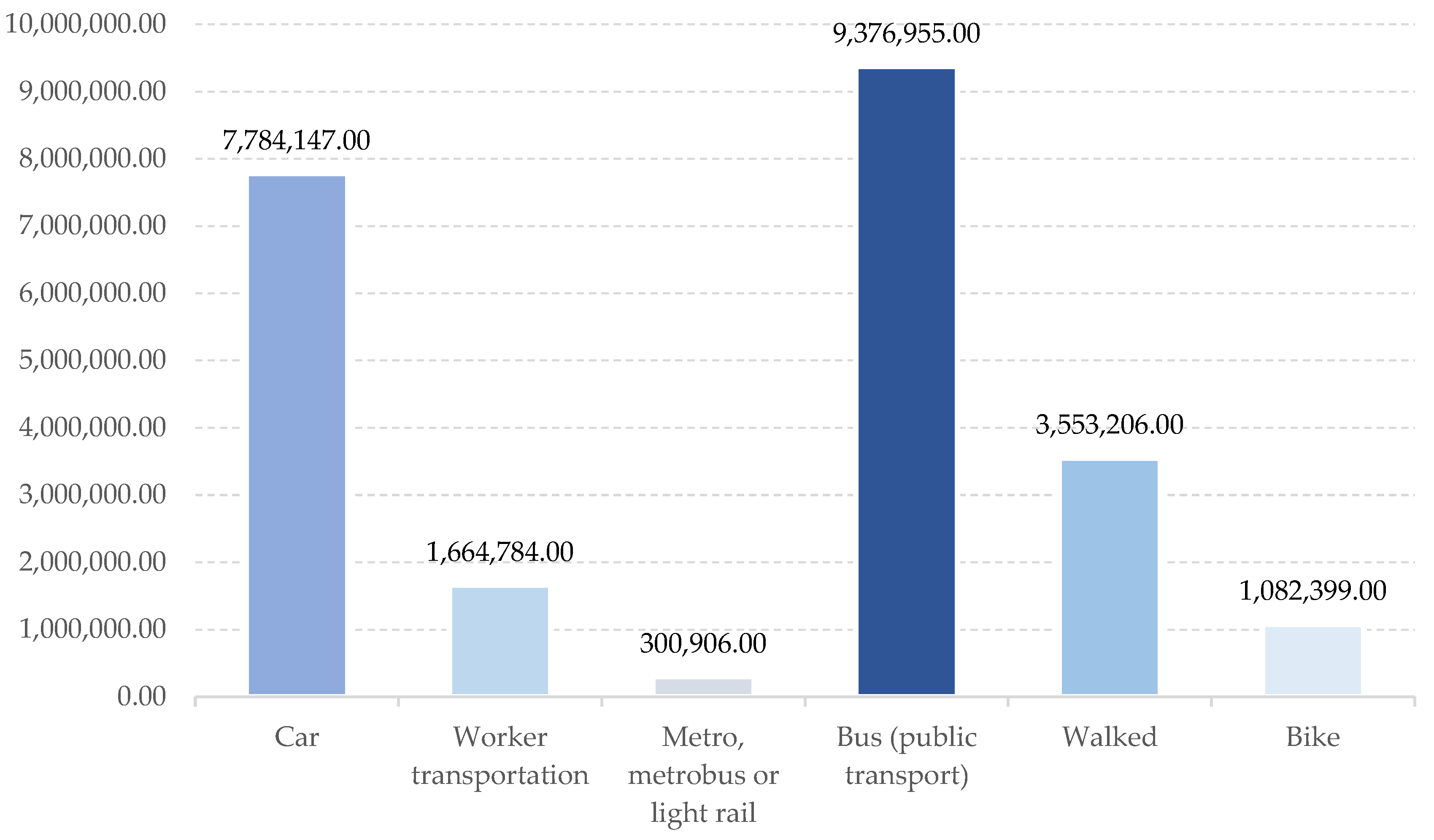
According to the 2015 INEGI Intercensal Survey, the occupied population (32%) took between 16 and 30 min to commute to and from work, while 10% took more than an hour [37]. This figure suggests that the occupied population of metropolitan municipalities travels over long distances, moves to a different municipality facing traffic or traffic jams, or uses more than one means of transport. Figure 3 shows the main means of transport used by the occupied population.

The occupied population in the 405 metropolitan municipalities amounted to 26,362,587 persons; of these, 2,206,686 (8%) did not require commuting to get to their workplace, while 24,155,901 (92%) did. As for the main means of transport used by the occupied population for commuting, 39.5% did it by bus or microbus (public transport); 33% by car; 14% walked; 7% by worker transportation; 4.6% by bicycle; and 1.3% by subway, Metrobus, or light train [37].

Table 2. Descriptive statistics.

Variable	Mean	Std. Dev.	Min.	Max.
$NOx$	1705.45	3839.53	1.51	50,534.38
$P{M}_{2.5}$	140.86	286.18	0.03	2785.67
$P{M}_{10}$	159.69	379.17	0.03	5357.04
$S{O}_2$	46.89	94.77	0.05	486.99
$CO$	7838.79	18,687.94	14.34	264,912.00
$COV$	860.99	1910.11	1.37	25,002.78
$N{H}_3$	16.64	50.02	0.02	867.84
Vehicle	43,843.76	97,874.81	1	708,548
Density	1015.90	2029.06	0.65	16,882.09
Bus vs. vehicle	0.70	-	0	1

shows the descriptive statistics of emissions, number of vehicles, population density, and a dichotomous variable that takes values of 1 for municipalities where the employed population uses the public bus more than the private car and zero otherwise (Bus vs. vehicle).

$CO$ and $NOx$ emissions showed the highest levels, while $N{H}_3$ and $S{O}_2$ showed the lowest levels.

Table 3. Emissions correlation matrix.

Variable	$\mathit{P}{\mathit{M}}_{\mathbf{2.5}}$	$\mathit{P}{\mathit{M}}_{\mathbf{10}}$	$\mathit{N}\mathit{O}\mathit{x}$	$\mathit{S}{\mathit{O}}_{\mathbf{2}}$	$\mathit{C}\mathit{O}$	$\mathit{C}\mathit{O}\mathit{V}$	$\mathit{N}{\mathit{H}}_{\mathbf{3}}$
$P{M}_{2.5}$	1.00
$P{M}_{10}$	0.96	1.00
$NOx$	0.91	0.94	1.00
$S{O}_2$	0.89	0.77	0.76	1.00
$CO$	0.87	0.93	0.98	0.73	1.00
$COV$	0.88	0.92	0.99	0.72	0.98	1.00
$N{H}_3$	0.78	0.90	0.93	0.52	0.96	0.94	1.00

shows the correlation matrix for pollutant emissions from 405 metropolitan municipalities. Emissions are highly correlated, with the highest correlation between $CO$ and $COV$ (0.98) and the lowest between $N{H}_3$ and $S{O}_2$ (0.52).

2.3. Principal Component Analysis

A principal component analysis was used to reduce pollutant emissions to a single dimension and derive an emissions index from factorial scores.

Table 4. Results of the principal component analysis of pollutant emissions.

	Initial Eigenvalues			Extraction Sums of Squared Loadings
	Total	% of Variance	Cumulative %	Total	% of Variance	Cumulative %
1	6.92	98.84	98.84	6.92	98.84	98.84
2	0.06	0.80	99.64
3	0.02	0.29	99.93
4	0.00	0.06	99.99
5	0.00	0.00	100.00
6	0.00	0.00	100.00
7	0.00	0.00	100.00

shows the total variance explained.

The Kaiser-Meyer-Olkin measure of sampling accuracy was 0.76 (p = 0.01), showing that the data was adequate for PCA. The first component accounted for 98.8% of the total variance in the data. To derive the index, the regression method was used as the criterion from which standardized factors were obtained.

Table 5. Component Matrix.

Z-Score	Component
	1	2
$N{H}_3$	0.82	−0.42
$COV$	0.86	−0.44
$NOx$	0.91	0.03
$CO$	0.82	−0.49
$S{O}_2$	0.81	0.17
$P{M}_{2.5}$	0.65	0.75
$P{M}_{10}$	0.73	0.63

shows the component matrix.

Equation (1) represent the linear combination of the pollutant emission variables in the first component from which the Polluting Emissions Index (PEI) scores were obtained:

$$PE{I}_i={\beta }_{N{H}_3}\left(\frac{X_{i,N{H}_3}-{\overline{X}}_{N{H}_3}}{S_{N{H}_3}}\right)+,\dots ,+{\beta }_{P{M}_{10}}\left(\frac{X_{i,P{M}_{10}}-{\overline{X}}_{P{M}_{10}}}{S_{P{M}_{10}}}\right)$$

(1)

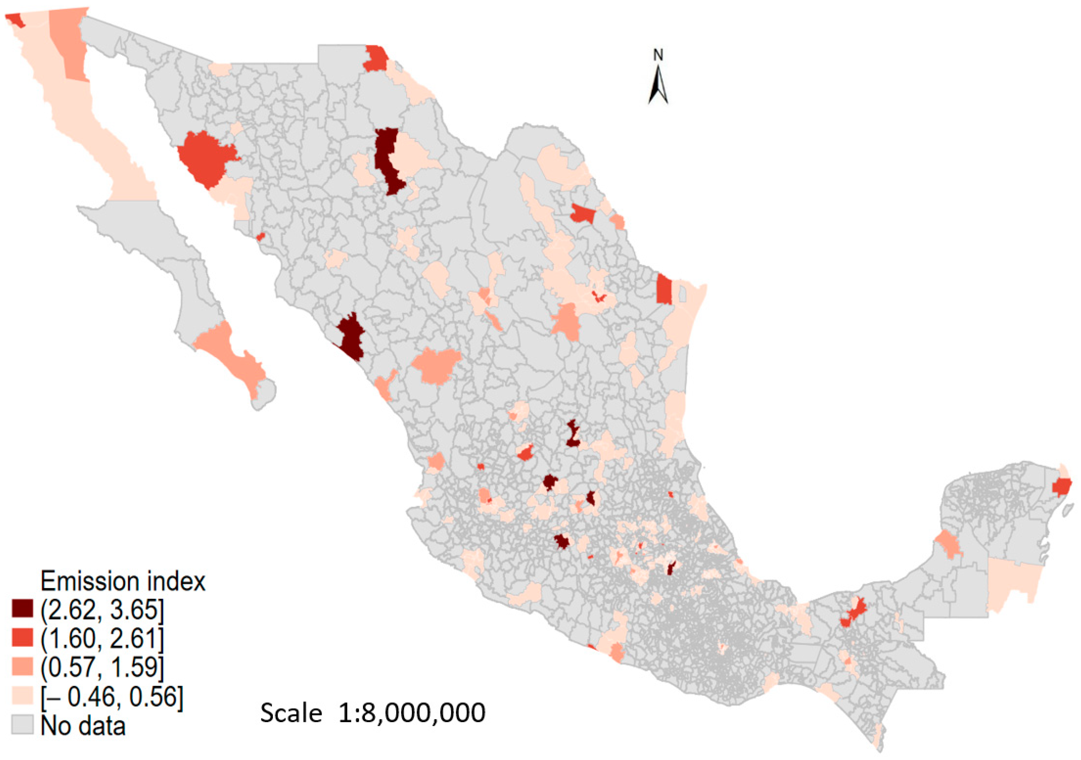
$PE{I}_i$ is the factorial score of the i-th municipality. The coefficients of the first component of the matrix of standardized coefficients $\beta$ in Equation (1) represent the relative weight of each standardized variable of polluting emissions with respect to the first component found, where: ${\beta }_{N{H}_3}=0.82; {\beta }_{COV}=0.86; {\beta }_{NOx}=0.91; {\beta }_{CO}=0.82; {\beta }_{S{O}_2}=0.81; {\beta }_{P{M}_{2.5}}=0.65; {\beta }_{P{M}_{10}}=0.73$. The terms in parentheses on the right side of Equation (1) correspond to the standardized values of the emissions in each municipality, specifically $X_{i,N{H}_3}$ is the value of $N{H}_3$ emissions in the i-th municipality; ${\overline{X}}_{N{H}_3}$ and $S_{N{H}_3}$ are the mean and standard deviation of the $N{H}_3$ emissions, respectively. The same notation is used in the other terms for each municipality and contaminant emissions. To visualize the spatial distribution of the emissions index, a georeferenced map was drafted from INEGI’s geostatistical framework for 2015 [37]. This allowed exploration of the spatial distribution of polluting emissions from mobile sources in metropolitan municipalities and their contiguity. The spatial distribution of the polluting emissions index by quantile is shown in Figure 4.

The main metropolitan areas of Mexico comprise municipalities with a high degree of urbanization, characterized by higher population densities in municipal heads or state capitals. The international empirical literature on pollutant gas emissions points to a spatial correlation because air pollution in a given locality depends not only on its own emission sources but also on pollutant emissions released in adjacent locations. A spatial autocorrelation analysis was performed to assess this phenomenon.

2.4. Exploratory Spatial Autocorrelation Analysis

To confirm the absence of a random spatial pattern in mobile emission levels of pollutant gases and the number of vehicles, an exploratory analysis was performed using Moran’s I, the statistical formula and statistical test of which are described as [9,38]:

$$I=\frac{N}{W} \frac{{{\displaystyle \sum }}_i{{\displaystyle \sum }}_j{w}_{ij}\left(x_i-\overline{x}\right)\left(x_j-\overline{x}\right)}{{{\displaystyle \sum }}_i{\left(x_i-\overline{x}\right)}^2}$$

(2)

$$Z-score=\frac{1-E\left(I\right)}{\sqrt{Var\left(I\right)}}$$

(3)

$$E\left(I\right)=-1/\left(N-1\right)$$

(4)

$$V\left(I\right)=E\left(I^2\right)-E{\left(I\right)}^2$$

(5)

where $N$ is the total number of municipalities in metropolitan areas; $W$ corresponds to the total number of neighborhoods; $x_i$ and $x_j$ are $NOx$ emissions from municipalities $i$ and $j$, respectively; $\overline{x}$ corresponds to average emissions. The matrix of spatial weights $W_{ij}$, is defined as follows [39]:

$$W=\left[\begin{array}{ccc}{w}_{11}& \cdots & w_{n1}\\ ⋮& \ddots & ⋮\\ w_{1n}& \cdots & w_{nn}\end{array}\right]$$

(6)

where $w_{ij}$ is defined as follows:

$$w_{ij}=\{\begin{array}{c}1 if i \in n_i\\ 0 otherwise\end{array}$$

(7)

where $n_i$ is the set of neighbors of the location $i$, so that $w_{ii}=0$. Separately, the standardized matrix by row from which the product matrix is obtained is defined as follows:

$$w_{ij}^{*}=\frac{w_{ij}}{{{\displaystyle \sum }}_{j=1}^n{w}_{ij}};w_{ij}^{*}\in W^{*}$$

(8)

The product matrix is defined as:

$$L\left(y\right)=W\times Y$$

(9)

Moran’s index ranges between −1 and +1: values close to 1 indicate strong spatial agglomeration, i.e., positive spatial autocorrelation. An index value close to 0 indicates a random spatial pattern, i.e., no spatial correlation. A value close to −1 indicates a scattered pattern with dissimilarity in the spatial characteristics, i.e., negative autocorrelation [11].

To conduct spatial autocorrelation tests, index values must be standardized to obtain the Z-score. Equations (4) and (5) correspond to the expected value and variance of Moran’s index, respectively. The p-values to determine the statistical significance of Moran’s Index are as follows: (1) $\left|Z\right|>1.96$ or $p<0.05,$ implies the rejection of the null hypothesis at 95% confidence that the residues of the adjusted regression considering Moran’s Index as the slope of the equation are Independent and Identically Distributed (i.i.d.); (2) $\left|Z\right|>2.58$ or $p<0.01,$ lead to the rejection of the null hypothesis at 99% confidence [9].

The absence of spatial autocorrelation was corroborated using Moran’s test. To this end, Moran’s index values were standardized by obtaining Z-scores, with which the null hypothesis of randomness or spatial independence was contrasted against the hypothesis of spatial autocorrelation. The results of the Moran’s test are shown in

Table 6. Results of Moran’s I test.

Variables	Moran’s I Statistic	Expected Value	Standard Deviation	Z	p-Value
$\ln (NOx$)	0.05	−0.002	0.01	4.97	0.00
ln(vehicles)	0.08	−0.002	0.01	7.79	0.00

.

Moran’s Index values of 0.05 for Nitrogen Oxide concentrations and 0.08 for the number of vehicles suggest a random spatial pattern. However, the results of the individual Moran’s test led to the rejection of the null hypothesis of absence of autocorrelation at a 99% confidence level. To explore whether the errors in the regression estimation between $NOx$ and the number of vehicles are i.i.d., a first-order binary spatial continuity matrix $W$ was constructed. The estimated ordinary least squares (OLS) model was as follows:

$$\ln (NO{x}_i)={\beta }_0+{\beta }_1\ln \left(vehicl{e}_i\right)+{\epsilon }_i$$

(10)

$${\epsilon }_i=\lambda W{\mu }_i+{\mu }_i$$

(11)

where $\ln (NO{x}_i)$ is the natural logarithm of nitrogen oxide emissions; $\ln \left(vehicl{e}_i\right)$ is the natural logarithm of number of vehicles in circulation; $\lambda$ is the spatial autocorrelation coefficient; ${\epsilon }_i$ is the error assumed to follow a normal distribution with zero mean and constant variance $~N\left(0,{\sigma }^2\right)$, and the null hypothesis to assess is $H_0:$ the residuals are i.i.d.

2.5. Spatial Model Selection Criteria

The methodological criterion for identifying the appropriate spatial model specification was based on a general model, following Arbia [39]. The initial spatial model is as follows:

$$y=\rho Wy+X\beta +WX\theta +u\hspace{1em} \left|\rho \right|<1$$

(12)

$$u=\lambda Wu+\epsilon \hspace{1em}\hspace{1em}\hspace{1em}\hspace{1em}\hspace{1em}\hspace{1em}\hspace{1em}\lambda <1$$

(13)

where $X$ is a matrix of non-stochastic regressors; ${\beta }_1$, ${\beta }_2$, and $\rho$ and $\lambda$ are the estimate parameters; $\epsilon |X\approx i.i.d.N\left(0,{\sigma }_{\epsilon }^2{I}_n\right)$ is the stochastic error; $\theta$ is the parameter of the explanatory variables with spatial lags and $W$ is the matrix of spatial weights previously described in Section 2.4.

This general specification can be reduced to a Spatial Durbin Model (SDM) if $\theta \ne 0$, $\rho \ne 0,$ and $\lambda =0$, while if $\theta =0$, $\rho =0$, and $\lambda \ne 0$, the general specification would collapse to a Spatial Error Model (SEM). If $\theta =0$, $\rho \ne 0$, and $\lambda =0$, the specification would be reduced to a Spatial Lag Model (SLM) of the dependent variable $NOx$ Emissions; if $\theta \ne 0$, $\rho =0$, and $\lambda =0$, the specification could be reduced to a Spatial Lag Model (SLX) of independent variables [34].

2.6. Spatial Model Specification

Following Arbia [39], a general spatial model was estimated considering both global effects and the effects of spatial dependence on errors:

$$\begin{gathered} \ln (NO{x}_i)={\beta }_0+\rho W\ln (NO{x}_i)+{\beta }_1\ln \left(vehicl{e}_i\right)+{\beta }_2\left(Bus vs vehicle\right)+{\beta }_{3}ln\left(density\right) \\ +{\theta }_{1}Wln\left(vehicl{e}_i\right)+{\theta }_{2}W\left(Bus vs vehicle\right)+{\theta }_{3}Wln\left(density\right)+{\mu }_i \left|\rho \right|<1 \end{gathered}$$

(14)

$${\mu }_i=\lambda W{\mu }_i+{\epsilon }_i \left|\lambda \right|<1$$

(15)

where $\ln (NO{x}_i)$ is the natural logarithm of the of nitrogen oxide emissions (tons per year) for the i-th metropolitan municipality; $W$ is the matrix of spatial weights or first-order binary contiguity, which takes values of 1 for metropolitan municipalities sharing common borders and values of zero otherwise. The independent variables correspond to the natural logarithm of the number of vehicles, population density, and a variable Bus vs. vehicle that takes values of 1 for metropolitan municipalities where the use of buses (public transport) is higher than the use of private cars by the occupied population; $W\ln \left(NOx\right)$ is the variable dependent with spatial lags according to the spatial weight matrix; $W\ln \left(vehicle\right)$ is the explanatory variable of the natural logarithm of the number of vehicles with a spatial lag according to $W$; and $W\ln \left(density\right)$ is the logarithm of the spatially weighted population density according to $W$. $W\ln \left(Bus vs vehicle\right)$ corresponds to Bus vs. vehicle, which takes values of 1 for metropolitan municipalities where the use of buses (public transport) is higher than the use of private cars by the occupied population, weighted according to the contiguity matrix $W$; $\rho$ is the spatial autocorrelation coefficient of the spatially lagged dependent variable; $\theta$ corresponds to the spatial autocorrelation coefficient of the natural logarithm of the number of vehicles; $\lambda$ is the spatial autocorrelation coefficient of the error; $W\mu$ is the spatially lagged error considering the matrix of spatial weights; and $\epsilon$ is the stochastic error $\epsilon |X\approx i.i.d.N\left(0,{\sigma }_{\epsilon }^2{I}_n\right)$, with $X$ as the matrix of non-stochastic regressors.

3. Results

The results of the estimation of the model are shown in

Table 7. Results of model with dependent variable $\ln$ ($NOx$).

Variable	OLS		SDM
	Coefficient	p-Value	Coefficient	p-Value
ln(vehicle)	0.33	0.00	0.40	0.00
Bus vs. vehicle	−0.80	0.00	−0.59	0.00
ln(density)	0.15	0.00	0.11	0.01
Wln(vehicle)			−0.37	0.00
WBus vs. vehicle			−0.40	0.33
Wln(density)			0.05	0.73
$\rho$			0.54	0.00
$\lambda$			−0.28	0.22
Constant	3.44	0.00	2.84	0.00
$R^2$	0.40		0.42
Moran’s test	11.28	0.00
Wald test			27.84	0.00

.

The coefficients of the OLS model were statistically significant according to the p-value, with a goodness of fit of 40%. However, the results of Moran’s test led to the rejection of the null hypothesis (i.e., errors are independent and identically distributed), so the alternative hypothesis of spatial dependence was accepted. As for the results of the initial general specification, the p-value of the spatial error parameter revealed no significant spatial effect on the error $(\lambda =0$). The spatially weighted lag parameter of the endogenous variable was statistically significant at 99% confidence $\left(\rho \ne 0\right)$. Of the independent variables with weighted spatial lags, only the logarithm of the number of vehicles was statistically significant at 1% significance $\left({\theta }_1\ne 0\right)$. The above indicates that the estimated general model is simplified to a Spatial Durbin Model (SDM), suggesting global and local spillover effects $\left[W\ln \left(NOx\right); W\ln \left(vehicl{e}_i\right)\right]$. The global effect of $NOx$ emissions can be identified by assuming an initial increase in $NOx$ emissions in ${\beta }_{ik}$ units, which will lead to a new increase from the change in adjacent metropolitan municipalities captured by the endogenous term $\rho W\ln (NO{x}_i)$. This implies that in each i-th metropolitan municipality, there will be a new impact equal to $0.54{\displaystyle \sum }_{j=1}^{405}{W}_{ij}{\beta }_{jk}$ units. This produces a dynamizing process that will be diluted through convergence, provided $\left|\rho \right|<1$, which, for the purposes of this study, which yielded a value of 0.54. According to Arbia [39], the constraints on the parameters $\rho$ and $\lambda$ are maintained when $W$ is standardized by rows (as defined in Equation (8)). The local effect of the number of vehicles can be identified by assuming an increase in the number of vehicles in the neighboring $J$ of the municipality $i$, with an impact equal to ${\displaystyle \sum }_{j=1}^{405}{W}_{ij}{\theta }_{jk}$. This spatial effect is deemed local, as it does not cause a dynamizing effect, such as the one produced by $\rho$ [40].

Interpreting the results of the effects of the spatial spillover of $NOx$ emissions, number of vehicles, population density, and use of public transport over private cars by the occupied population requires estimating the total effect of municipalities adjacent to each location, given the magnitude of the coefficients of the explanatory variables that consider the contiguity matrix. The total effect can be split into direct and indirect effects. Direct effects capture the change in the dependent variable, i.e., $NOx$, derived from changes in the explanatory variables such as ln(vehicle), Bus_vs_vehicle, and ln(density), and can be expressed from partial derivatives $\left(\partial NO{x}_i/\partial X_{ik}\right)$; indirect effects are obtained from cross-derivatives $\left(\partial NO{x}_i/\partial X_{Jk}\right)$; therefore, the total effect can be expressed as: $\left(\partial NO{x}_i/\partial X_{ik}\right)+\left(\partial NO{x}_i/\partial X_{Jk}\right)$ [35]. Because marginal effects are not unique to all localities, LeSage and Pace [40] proposed a summary metric based on the average of the main diagonal elements of the partial derivative matrix. According to LeSage [41], the impacts estimated from cross-sectional partial derivatives in neighboring localities interpreted as indirect effects or spillover effects should take time. However, in cross-sectional models (as in the present study), these effects should be interpreted as comparative static changes that will arise in the dependent variable as the relationship between variables evolves toward a new steady-state equilibrium.

Direct and Indirect Effects

The direct, indirect, and overall effects of the Spatial Durbin Model are shown in

Table 8. Spatial spillover effects.

Direct Effect	Coefficient	Standard Error	Z	p-Value
ln(vehicle)	0.40	0.03	13.57	0.00
Bus vs. vehicle	−0.63	0.18	−3.47	0.00
ln(density)	0.12	0.04	2.80	0.00
Indirect Effect	Coefficient	Standard Error	Z	p-value
ln(vehicle)	−0.11	0.04	−3.17	0.00
Bus vs. vehicle	−0.57	0.36	−1.6	0.11
ln(density)	0.09	0.11	0.84	0.40
Total Effect	Coefficient	Standard Error	Z	p-value
ln(vehicle)	0.28	0.04	6.81	0.00
Bus vs. vehicle	−1.21	0.39	−3.10	0.00
ln(density)	0.21	0.11	1.91	0.06

.

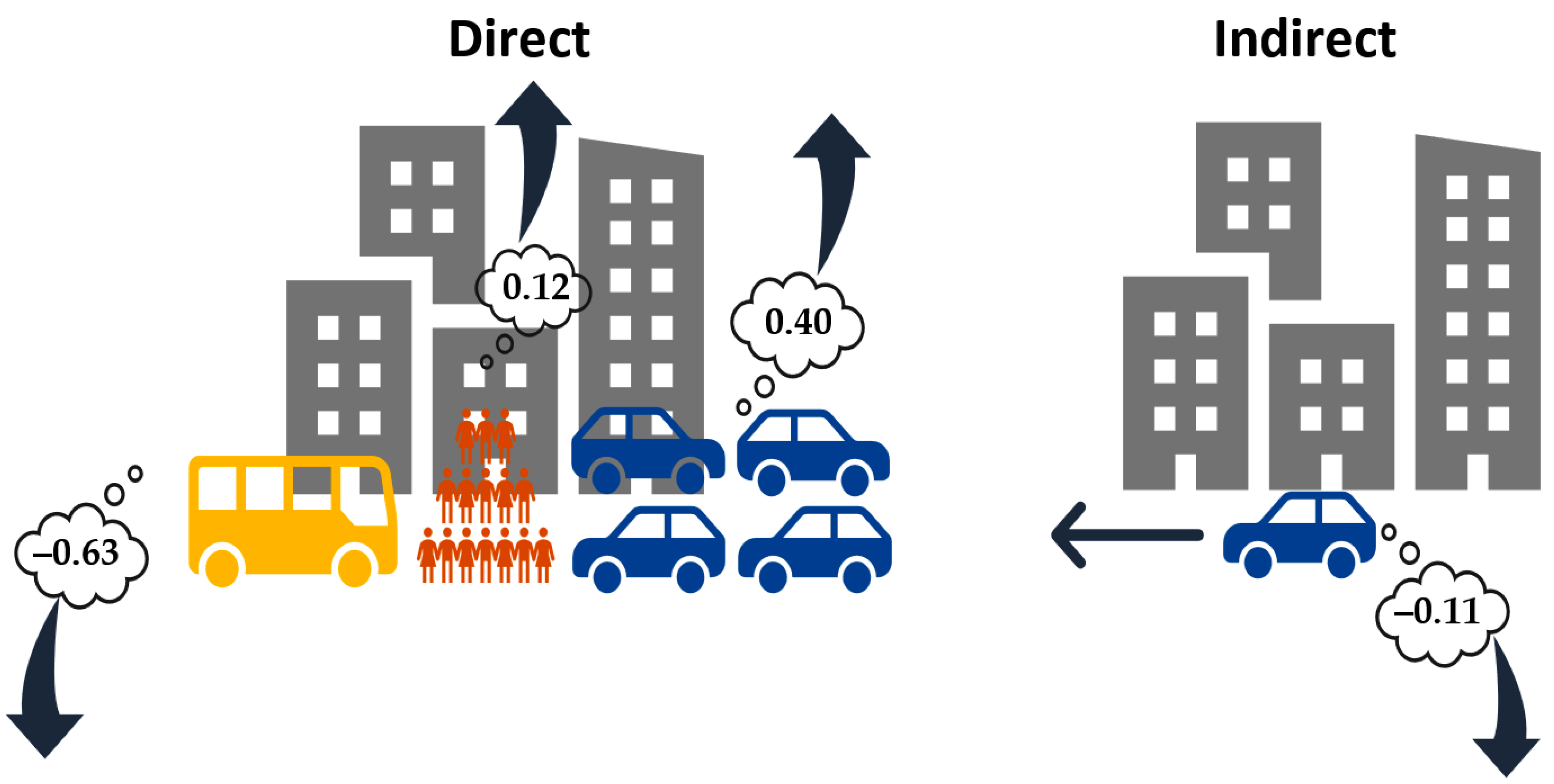
The number of vehicles has direct positive effects on $NOx$ emissions in metropolitan municipalities. A 1% increase in the number of vehicles in a metropolitan municipality translates into an average increase of 0.40% in $NOx$ emissions. An important aspect is that the greater use of public transport by the occupied population (instead of private cars) has statistically significant direct negative effects. On average, a municipality with greater use of public transport by the occupied population has lower $NOx$ emissions (−0.63%) than municipalities where the use of private cars is greater than the use of public transport. The population density in these municipalities has positive direct and statistically significant effects on nitrogen oxide emissions. The direct effect of population density on emissions can be interpreted as the change in emission levels associated with a 1% increase in population density. Thus, on average, a 1% increase in population density in a metropolitan municipality would lead to a 0.12% increase in nitrogen oxide emissions.

As for the indirect effects of independent variables in adjacent municipalities on a specific municipality, we found that only the number of vehicles in adjacent municipalities has negative and statistically significant impacts. The indirect marginal effect of the number of vehicles in adjacent metropolitan municipalities on emissions in a given municipality can be interpreted according to the results as follows: on average, a 1% increase in the number of vehicles in adjacent municipalities would lead to a 0.11% decrease in $NOx$ emissions in a given metropolitan municipality.

Greater urban growth and economic dynamism in the CBDs of metropolitan municipalities favor increases in the number of vehicles in circulation that generate vehicular traffic, an increase in local $NOx$ emissions and lower $NOx$ emissions in neighboring municipalities with different urban environment characteristics. This generates negative spillover effects on $NOx$ emissions. Figure 5 shows a flowchart of the direct and indirect spatial effects of the number of vehicles, population density, and greater use of buses with respect to private cars on $NOx$ emissions.

The total effect of the number of vehicles in a given municipality and adjacent municipalities on $NOx$ emissions is positive and statistically significant. In other words, a 1% increase in the number of vehicles in a given municipality and adjacent municipalities leads to a 0.28% increase in $NOx$ emissions, on average. Our results indicate that the greater use of buses or public transport versus private cars by the occupied population in a given municipality and its neighboring municipalities has an overall negative effect, which is statistically significant at a 99% confidence level. In other words, a municipality with greater use of public transport by the occupied population than private cars, together with adjacent municipalities with the same mobility pattern, produces 1.21% lower $NOx$ emissions than municipalities with greater use of private cars. The total effect of population density on emissions was positive and statistically significant only at the 90% confidence level; accordingly, the data used in this study provide weak evidence of the overall effect of population density on $NOx$ emissions. The data set used in PCA as well as OLS and SDM estimations is available as supplementary materials.

4. Discussion

According to the literature survey conducted herein on the global and local effects of the drivers of pollutant gas emissions, this work is the first to analyze the direct and indirect effects of recorded vehicle traffic (number of vehicles in circulation) in the main metropolitan areas of Mexico. To this end, we used the 2016 National Inventory and Criteria for Pollutant Gas Emissions, the number of registered cars in circulation at the national level in 2016, and information on urban mobility at the municipal level. According to the results of the principal component analysis, the seven pollutant gases, namely $CO$; $P{M}_{2.5}; P{M}_{10}$; $N{H}_3$; $VOCs$; $NOx$ and $S{O}_2$ can be reduced by a single factor from the linear combination obtained. This allowed us to obtain the factorial scores that make up the emissions index and to construct a map with the spatial distribution of the emissions index by quantiles. This revealed a certain degree of heterogeneity in the emissions index, with higher levels in head municipalities and state capitals and lower levels in neighboring municipalities.

The spatial effects of the number of vehicles in circulation, the use of public transport by the occupied population, and population density were estimated using an SDM model. Direct and indirect effects were estimated using the delta method. All three variables showed significant direct effects. As for indirect effects, only the number of registered cars in circulation showed spatial spillover effects on $NOx$ emissions, which are statistically significant (p < 1%).

The number of vehicles had positive direct and negative indirect effects on $NOx$ emissions. This is consistent with the conclusions reported in previous studies [10,11,15,16] indicating that great traffic intensity in a given locality and adjacent areas increases local emissions. A 1% increase in the number of vehicles in circulation causes a 0.40% increase in local $NOx$ emissions. On the other hand, a 1% increase in the number of registered cars in circulation in adjacent municipalities will decrease $NOx$ emissions by 0.11% in the respective local municipality. Considering the overall effect of direct and indirect emissions, it was found that the indirect negative effects of the number of vehicles in circulation (−0.11%) are insufficient to compensate for the direct effect of the emissions released by the number of local vehicles in a given municipality. Therefore, the overall effect of the number of vehicles in circulation was 0.28%. This implies that a 1% increase in the number of vehicles in a given municipality and adjacent municipalities will lead to a 0.28% increase in $NOx$ emissions.

The Bus vs. car dichotomous variable, which takes values of 1 for municipalities with the highest use of public transport compared to cars by the occupied population and values of zero otherwise, resulted in negative direct effects, i.e., the increased use of public transport contributes to reducing local $NOx$ emissions. These results are consistent with the direct effects reported by Jia et al. [28] regarding the fact that the increase in the use of light rail reduces local emissions. However, unlike the study by Jia et al. [28], the effects of spatial spillover due to the greater use of urban public transport (bus) estimated in the present study were not statistically significant. Namely, this study only found that greater use of the bus compared to private cars reduces local $NOx$ emissions.

With regard to the impact of population density, the results of the present study indicate that the increase in population density leads to increased local emissions of nitrogen oxides $\left(NOx\right)$. These results are consistent with those reported by Yang et al. [10] for $C{O}_2$ concentrations. However, the indirect effects that would lead to spatial spillover were not significant in this study. The main limitations of this study are the absence of control variables on the age of private cars, and fuel quality (octane). However, this information is not available at the municipal level for the study period.

5. Conclusions

The present study surveyed the existing literature on the drivers of pollutant gas emissions in localities, cities, municipalities, and urban regions. The spatial impacts reported in previous studies are summarized. An index of pollutant gas emissions and a map of the spatial distribution per quantile were also generated. Using information from the 2015 Intercensal Survey, we analyzed the mobility of the occupied population by type of transport used and commute time to the workplace. The number of vehicles was described by unit type in Mexico from 1980 to 2018. A spatial autocorrelation analysis of $NOx$ emissions was performed. To this end, Moran’s index was calculated, and its statistical significance was tested. Then, a general spatial model was specified from which the SDM model was identified and confirmed as suitable for estimating global and local impacts, as noted in previous studies.

The results highlight the positive direct effects of the number of vehicles and population density, as well as the negative direct effects of the use of urban public transport, indicating that the increase in the number of registered vehicles in circulation and population density increases local $NOx$ emissions. On the other hand, the increase in the use of public transport as an alternative to private cars reduces the local emissions of $NOx$. The number of vehicles in circulation produced negative spatial indirect effects from the $NOx$ emissions of the contiguous metropolitan municipalities. This indicates that a greater flow of vehicular traffic in the Central Business Districts of the metropolitan areas has the effect of reducing $NOx$ emissions in neighboring municipalities with different characteristics of the built environment.

The contribution of this study was to provide empirical evidence of the direct and spatial spillover effects of the number of vehicles in circulation in Mexico. The results indicate that a 1% increase in the number of private vehicles in circulation has a direct effect of a 0.40% increase in $NOx$ emissions and a negative indirect effect by reducing emissions by 0.11% in neighboring municipalities. Another contribution was the measurement of the effect of greater use of public transport with respect to private cars on NOx emissions. In this regard, it was found that metropolitan municipalities where the employed population (workers) has a higher percentage of use of public transport with respect to the private car, on average, they have 63% less $NOx$ emissions. Additionally, positive spatial association patterns of $NOx$ emissions are identified. A greater relative use of the bus with respect to the private car presented a negative spatial association pattern in $NOx$ emissions. The univariate spatial association can be explicated in part by atmospheric transportation processes between neighboring municipalities, while the negative spatial association of $NOx$ emissions and the greater relative use of buses with respect to private cars reveals the importance of this type of transport in mobility between contiguous metropolitan municipalities. In this sense, this study contributes information about the impact on air pollution that greater use of alternative modes of transport to private cars in the main metropolitan areas of Mexico.

This study contributes to the specialized literature on air pollution with a spatial approach by analyzing the direct and indirect effects of population density and the relative use of buses with respect to private cars on $NOx$ emissions in Mexico. Likewise, this is the first study to measure local and spillover effects of population density and relative use of the bus on $NOx$ emissions, as well as the first in Latin America with this approach. These results can serve as a reference in Latin American countries with similar characteristics.

The conclusion is that the design of public policy programs aimed at reducing air pollution should be based on coordination between metropolitan municipalities, given the direct effects and spatial spillover effects of vehicle traffic on $NOx$ emissions in metropolitan municipalities in Mexico. One of the main constraints of the present study is that it does not include control variables, such as characteristics of old vehicles and their classification by type of fuel consumed, i.e., oil, diesel, hybrid, and electric. This type of information is unavailable at the municipal level for the study period. Another limitation of the study is that it does not include transport variables and atmospheric chemical reactions. Another limitation of this study is that the availability of information only allowed for a cross-sectional analysis. A next step in this line of research will be to select a large metropolitan area or megalopolis with a certain number of municipalities and generate these variables that allow for a longitudinal study of local direct effects and spatial spillovers of population density, number of vehicles, and relative use of public transport on air pollution. The next step in this study will be to analyze the effects of air pollution on the health of the population of these metropolitan areas.

References

1. Lehmann, P. Justifying a policy mix for pollution control: Are view of economic literature. J. Econ. Surv. 2012, 26, 71–97. [Google Scholar] [CrossRef]
2. Baiardi, D. Do sustainability energy policies matter for reducing air pollution? Energy Policy 2020, 140, 111364. [Google Scholar] [CrossRef]
3. Akimoto, H.; Tanimoto, H. Rethinking of the adverse effects of NOx-control on the reduction of methane and tropospheric ozone-Challenges toward a denitrified society. Atmos. Environ. 2022, 227, 119033. [Google Scholar] [CrossRef]
4. Finlayson-Pitts, B.J.; Pitts, J.N., Jr. Chemistry of the Upper and Lower Atmosphere; Academic Press: Cambridge, MA, USA, 2000. [Google Scholar] [CrossRef]
5. Akimoto, H. Atmospheric Reaction Chemistry; Springer: Berlin/Heidelberg, Germany, 2016. [Google Scholar] [CrossRef]
6. SEMARNAT. Inventario Nacional de Emisiones de Gases Contaminantes, Criterios 2016 (INEM). 2016. Available online: https://gisviewer.semarnat.gob.mx/wmaplicacion/inem/ (accessed on 8 October 2021).
7. Huang, H.-C.; Lin, F.C.-F.; Wu, M.-F.; Nfor, O.H.; Hus, S.-Y.; Lung, C.-C.; Chen, C.-Y.; Liaw, Y.-P. Association between chronic obstructive pulmonary disease and PM2.5 in Taiwanese nonsmokers. Int. J. Hyg. Environ. Health 2019, 222, 884–888. [Google Scholar] [CrossRef]
8. Alotaibi, R.; Bechle, M.; Marshall, J.D.; Ramani, T.; Zietsman, J.; Nieuwenhuijsen, M.J.; Khreis, H. Traffic related air pollution and the burden of childhood asthma in the contiguous United States in 2000 and 2010. Environ. Int. 2019, 127, 858–867. [Google Scholar] [CrossRef]
9. Wang, J.; Li, R.; Xue, K.; Fang, C. Spatio-Temporal Heterogeneity and Socioeconomic driving Factors of PM2.5 in Beijing-Tianjin-Hebei and Its Surroungding Areas. Atmosphere 2021, 12, 1324. [Google Scholar] [CrossRef]
10. Yang, W.; Wang, W.; Ouyang, S. The influencing factors and spatial spillover effects of CO2 emissions from transportation in China. Sci. Total Environ. 2019, 969, 133900. [Google Scholar] [CrossRef]
11. Diao, B.; Ding, L.; Su, P.; Cheng, J. The Spatial-Temporal Characteristics and Influential Factors of NOx Emissions in China: A Spatial Econometric Analysis. Int. J. Environ. Res. Public Health 2018, 15, 1405. [Google Scholar] [CrossRef]
12. Cheng, Z.; Li, L.; Liu, J. Identifying the spatial effects and driving factors of urban PM2.5 pollution in China. Ecol. Indic. 2017, 82, 61–75. [Google Scholar] [CrossRef]
13. Liu, X.; Xia, H. Empirical analysis of the influential factors of haze pollution in China—Based on spatial econometric model. Energy Environ. 2018, 30, 854–866. [Google Scholar] [CrossRef]
14. Wang, L.; Zhao, Z.; Xue, X.; Wang, Y. Spillover effects of railway and road on CO2 emissions in China: A spatiotemporal analysis. J. Clean. Prod. 2019, 234, 797–809. [Google Scholar] [CrossRef]
15. Ren, Y.; Ren, X.; Hu, J. Driving factor of China’s city-level carbon emissions from the perspective of spatial spillover effect. Carbon Manag. 2019, 10, 551–566. [Google Scholar] [CrossRef]
16. Qiang, W.; Lee, H.F.; Lin, Z.; Wong, D.W.H. Revisiting the impact of vehicle emissions and other contributors to air pollution in urban built-up areas: A dynamic spatial econometric analysis. Sci. Total Environ. 2020, 740, 140098. [Google Scholar] [CrossRef]
17. Chen, Y.; Whalley, A. Green infrastructure: The effects of urban rail transit on air quality. Am. Econ. J. Econ. Policy 2012, 4, 58–97. [Google Scholar] [CrossRef]
18. Du, Y.; Sun, T.; Peng, J.; Fang, K.; Liu, Y.; Yang, Y.; Wang, Y. Direct and spillover effects of urbanization on PM2.5 concentrations in China´s top three urban agglomerations. J. Clean. Prod. 2018, 190, 72–83. [Google Scholar] [CrossRef]
19. Lu, J.; Li, B.; Li, H.; Al-Barakani, A. Expansiono of city scale, traffic modes, traffic congestion, and air pollution. Cities 2021, 108, 102974. [Google Scholar] [CrossRef]
20. Song, L.; Jing, J.; Yan, Z.; Sun, C. Does government information transparency contribute to pollution abatement? Evidence from 264 Chinese cities. Environ. Sci. Pollut. Res. 2021, 29, 12853–12863. [Google Scholar] [CrossRef]
21. Yu, X.; Shen, M.; Shen, W.; Zhang, X. Effects of Land Urbanization on Smog Pollution in China: Estimation of Spatial Autoregressive Panel Data Models. Land 2020, 9, 337. [Google Scholar] [CrossRef]
22. Ding, X.; Cai, Z.; Xiao, Q.; Gao, S. A study on The Driving Factors and Spatial Spillover of Carbon Emission Intensity in The Yangtze River Economic Belt under Double Control Action. Int. J. Environ. Res. Public Health 2019, 16, 4452. [Google Scholar] [CrossRef]
23. Mamipour, S.; Beheshtipour, H.; Feshari, M.; Amiri, H. Factors influencing carbon dioxide emissions in Iran´s provinces with emphasis on spatial linkages. Environ. Sci. Pollut. Res. 2019, 26, 18365–18678. [Google Scholar] [CrossRef] [PubMed]
24. Ge, X.; Zhou, Z.; Zhou, Y.; Ye, X.; Liu, S. A spatial Panel Data Analysis of Economics Growth, Urbanization, and nitrogen oxide emissions in China. Int. J. Environ. Res. Public Health 2018, 15, 725. [Google Scholar] [CrossRef]
25. Xie, R.; Wei, D.; Han, F.; Lu, Y.; Fang, J.; Liu, Y.; Wang, J. The effect of traffic density on smog pollution: Evidence from Chinese cities. Technol. Forecast. Soc. Change 2019, 144, 421–427. [Google Scholar] [CrossRef]
26. Kutlu, L.; Wang, R. Greenhouse Gas Emission Inefficiency Spillover Effects in European Countries. Int. J. Environ. Res. Public Health 2021, 18, 4479. [Google Scholar] [CrossRef]
27. Yu, X.; Wu, Z.; Zheng, H.; Li, M.; Tan, T. How urban agglomeration improve the emission efficiency? A spatial econometric analysis of the Yangtze River Delta urban agglomeration in China. J. Environ. Manag. 2020, 263, 110061. [Google Scholar] [CrossRef] [PubMed]
28. Jia, R.; Shao, S.; Yang, L. High-speed rail and CO2 emissions in urban China: A spatial difference-in-differences approach. Energy Econ. 2021, 99, 105271. [Google Scholar] [CrossRef]
29. Li, J.; Huang, X.; Chuai, X.; Yang, H. The impact of land urbanization on carbon dioxide emissions in the Yangtze River Delta, China: A multiscale perspective. Cities 2021, 116, 103275. [Google Scholar] [CrossRef]
30. Wu, X.; Gao, M.; Guo, S.; Li, W. Effects of environmental regulation on air pollution control in China: A spatial Durbin Econometric analysis. J. Regul. Econ. 2019, 55, 307–333. [Google Scholar] [CrossRef]
31. Feng, T.; Du, H.; Lin, Z.; Zuo, J. Spatial spillover effects of environmental regulations on air pollution: Evidence from urban agglomerations in China. J. Environ. Manag. 2020, 272, 110998. [Google Scholar] [CrossRef] [PubMed]
32. Zhang, L.; Wang, Q.; Zhang, M. Environmental regulation and CO2 emissions: Based on strategic interaction of environmental governance. Ecol. Complex. 2021, 45, 100893. [Google Scholar] [CrossRef]
33. Zhong, S.; Li, J.; Zhao, R. Does environmental information disclosure promote sulfur dioxide (SO2) remove? New evidence from 113 cities in China. J. Clean. Prod. 2021, 299, 126906. [Google Scholar] [CrossRef]
34. Zhong, S.; Bushell, M. Impact of the built environment on the vehicle emission effects of road pricing policies: A simulation case study. Transp. Res. Part A Policy Pract. 2017, 103, 235–249. [Google Scholar] [CrossRef]
35. Sun, Z.Q.; Sun, T. The impact of multi-dimensional urbanization on China´s carbon emissions based on the spatial spillover effect. Pol. J. Environ. Stud. 2020, 29, 3317–3327. [Google Scholar] [CrossRef]
36. INEGI. Vehículos de Motor Registrado en Circulación, año 2016. 2021. Available online: https://www.inegi.org.mx/programas/vehiculosmotor/ (accessed on 8 October 2021).
37. INEGI. Encuesta Intercensal 2015. Available online: https://www.inegi.org.mx/programas/intercensal/2015/ (accessed on 8 October 2021).
38. Siabato, W.; Guzmán-Manrique, J. La autocorrelación espacial y el desarrollo de la geografía cuantitativa. Cuad. Geogr. Rev. Colomb. Geogr. 2019, 28, 1–22. [Google Scholar] [CrossRef]
39. Arbia, G. A Primer for Spatial Econometrics with Applications in R; Springer: Berlin/Heidelberg, Germany, 2014. [Google Scholar] [CrossRef]
40. Lesage, J.; Pase, K.R. Introduction to Spatial Econometric; CRC Press, Taylor & Francis Group: Boca Raton, FL, USA, 2009. [Google Scholar]
41. LeSage, J.P. What Regional Scientists Need to Know about Spatial Econometrics. Rev. Reg. Stud. 2014, 44, 13–32. [Google Scholar] [CrossRef]
Figure 1. Number of registered cars in circulation at the national level from 1980 to 2019.
Atmosphere 13 01191 g001
Figure 2. Distribution of commute time of the occupied population.
Atmosphere 13 01191 g002
Figure 3. Main means of transport used by the occupied population.
Atmosphere 13 01191 g003
Figure 4. Emissions index for 405 metropolitan municipalities in Mexico in 2016.
Atmosphere 13 01191 g004
Figure 5. Flow diagram of direct and indirect spatial effects of the number of vehicles, population density, and greater use of buses with respect to private cars on N O x emissions.
Atmosphere 13 01191 g005