Abstract
The construction of protective forests in Nursultan is key to reducing near-surface wind speeds and snowstorm effects in urban areas. This study analyzed the effects of the number of plant rows and spacing of the shelterbelts on the flow field around protective forests to evaluate the wind protection benefits of the existing configuration of the shelterbelt in Nursultan and guide the construction of protective forests. We measured the airflow fields of four shelterbelts with different numbers of rows, seven double pure shelterbelts, and double mixed shelterbelts of arbors and shrubs with different spacings. The results showed that the airflow field around the shelterbelts can be divided into five characteristic regions based on shelter efficiency: a deceleration region before the shelterbelt, acceleration region above the canopy, strong deceleration region in the canopy layer, deceleration region behind the shelterbelt, and recovery region behind the shelterbelt. In terms of windproof ability, the wind protection benefits of a shelterbelt with six rows are the best in a single shelterbelt. Behind the shelterbelt, the wind protection benefits of double pure shelterbelts are greater than that of double mixed shelterbelts of arbor and shrub. On the contrary, the windbreak benefits of the latter are stronger than those of the former between the two shelterbelts.
1. Introduction
A protective forest, also called a shelterbelt, windbreak, or shelter forest, is a forest with the basic management goal of providing an ecological services function. They are planted in ecologically fragile areas or in the vicinity of protected objects. A windbreak is defined as any structure that reduces wind speed [1]. Windbreaks can be a single element or a system of elements and can reduce wind speed, windward and leeward, based on their position regarding the airflow [2]. The results of previous studies showed that the selection of tree species and configuration of the shelterbelt structure are key to constructing shelterbelts as they determine whether the shelterbelt can give full play to its windproof efficiency [3,4,5,6]. A reasonable forest belt structure can effectively enhance the protective effect [5,7,8,9,10,11]. Therefore, it is important to understand the shelter efficiencies of shelterbelts with different configurations to select the best afforestation mode.
A shelterbelt typically comprises one or more rows of plants arranged in a certain pattern [12]. Vegetation affects the airflow dynamics by extracting momentum from the flow [13]. The wake zones of multiple plants in the shelterbelt overlap in skimming flow, resulting in the distribution of the airflow field around the shelterbelt, which differs from that around a single plant [14,15,16]. The plant height, porosity, number of rows in a forest belt, arrangement, distribution of vegetation, and wind angle affect the characteristics of the airflow field around the vegetation [2,14,17]. The taller the vegetation, the longer the protection distance from the forest belt [18]. Porosity determines the extent of wind velocity reduction, turbulence level, and sheltered area in the lee of the windbreaks [19,20]. Porosity is influenced by row numbers, the spacing between rows, and the amount and density of leaves and branches of vegetation [21]. At a higher porosity, airflow encounters less resistance when passing through plants and the reduction in wind speed is smaller. At a very low porosity, airflow encounters greater resistance and is lifted upwind of the vegetation, forming strong eddy currents in the lee of the vegetation, which shortens the protection distance [22]. Gao et al. [23] showed that the desirable porosity level to reduce wind speed is 25–40% and other studies have suggested ranges from 20 to 40% [17,24,25,26]. In contrast, Brandle et al. [27] and Yang et al. [28] suggested that a porosity between 40% and 50% is the most efficient. The higher the shelterbelts and the more rows of plants they have, the greater their shelter efficiency [18,29]. However, the relationship between the shelter efficiency and row number is nonlinear [30]. In addition, the cross-sectional shape of the shelterbelt also affects the downwind airflow field. Research shows that the geometric shape and density of plants have great effects on wind profiles [31,32]. Liu et al. [30] used computational fluid dynamics to simulate the airflow and turbulence around trees with different geometric shapes and found that a plant canopy that was large at the bottom and small at the top exhibited better shelter efficiency. Miri et al. [33] found that the porosity and frontal area of the shelterbelt would change under high wind speed. This change is determined by plant structure and influences the amount of momentum extracted from the airflow. Woodruff et al. [34] found that a rectangular or trapezoidal cross section is better than other shapes. A mixed composite shelterbelt comprising trees, shrubs, and grass may have a better shelter efficiency due to the alteration of the cross-sectional shape of the shelterbelt [18,35,36].
In addition, understanding the distributions of airflow fields around shelterbelts is essential for analyzing the area protected by protective forests. Based on the different shelterbelt configurations, the previous delineation of the typical airflow field around the shelterbelt differs. Based on the division of airflow fields near fences proposed by Judd et al. [37], Leenders et al. [38] divided the airflow fields around single plants into several categories: flow-in, permeate, shift, station, mix, and recovery regions. Other scientists divided airflow fields around plants into the following categories: mild deceleration area in the upwind region [18], acceleration areas on both sides [39,40], and wake deceleration area in the downwind region [40,41,42]. In addition, Fu et al. [43], Cheng et al. [14], and Miri et al. [44] also observed deceleration and acceleration areas around vegetation. The flow field around the forest zone was divided into five typical regions by Ma et al. [4]: an acceleration region above the canopy, large deceleration region within the canopy and leeward of the windbreaks, and a local acceleration region below the canopy of the first few rows. Belcher et al. [45] demonstrated that the turbulent flow over and through a vegetative canopy can be divided into seven regions: impact region, adjustment region, canopy interior, canopy shear layer, roughness change region, exit region, and far wake.
The Nursultan Green Ring Project aims to reduce the near-surface wind speed and effects of snowstorms on the city by planting original natural grassland between arbors and shrubs to improve the ecological environment. By 2018, shelterbelts had been planted over 86,800 hectares. However, further expansion is necessary and shelterbelts are expected to cover 300,000 hectares by 2030. Kabanova et al. [46] suggested that the conditions of Nursultan are unfavorable for green construction because of the continental climate, harsh wind regime, and low-productive soils with low forest vegetation qualities. Nursultan is a desert grassland area; therefore, careful planting is required to design a shelterbelt configuration that achieves the project’s purpose with the lowest number of trees and low water consumption. The airflow field, effective protection distance, and windbreak effect under different shelterbelt structures have been analyzed in previous studies. However, it remains unclear how many rows produce the best windproofing effect, and there is no consensus on the difference between pure arbor forests and combined arbor and shrub forests with different belt spacings. Given the large planting area and the diverse shelterbelt configuration in Nursultan, we conducted wind tunnel experiments to evaluate the wind protection effectiveness of artificial protective forests. We measured the airflow field for four single shelterbelts with different rows, seven pure shelterbelts with different spacings, and seven combined arbor–shrub shelterbelts with different spacings to determine the effects of the spacing and number of rows on the airflow field as well as the differences in the protection efficiencies of single- and mixed-species shelterbelts. The aim was to use a wind tunnel test to determine the optimal number of rows and spacing to ensure the highest efficiency for the shelterbelt. The results provide theoretical guidance for the implementation of the Ring Shelterbelt in Nursultan, especially for the species allocation in different regions.
2. Materials and Methods
2.1. Experimental Setup and Materials
Our experiment was conducted in an indoor wind tunnel at the Xinjiang Institute of Ecology and Geography of the Chinese Academy of Sciences. The wind tunnel was a direct current blowing wind tunnel with a total length of 16.2 m and an experimental section of 8 m. The cross section was 1.3 × 1.0 m. A sidewall diffusion-type structure was used and the diffusion angle of each sidewall was 0.2°. A frequency conversion motor was used to adjust the wind speed by altering the current frequency. The wind speed level could be continuously adjusted from 0 to 20 m·s−1 based on the experimental requirements [47]. A schematic of the wind tunnel structure is shown in Figure 1.
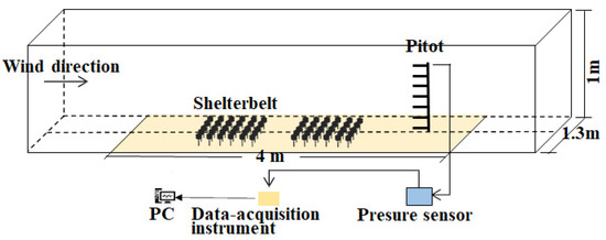
Figure 1.
Schematic diagram of the experimental wind tunnel.
We measured the wind fields of three shelterbelt types (Figure 2a). During the wind tunnel test, the pitot tube was erected at the center of the tunnel cross section along the axial direction of the wind tunnel test section to measure the flow field (pitot tubes were erected at nine heights: 1, 2, 3, 5, 7, 10, 15, 30, and 50 cm). Wind speeds of 6, 7, and 8 m·s−1 were selected for the observations. The acquisition frequency of the wind tunnel system simulation software was 1 s acquisition and recording, followed by the measurement of wind speed at each observation point for 3 min, after which the average value of the last 20 data points recorded after the wind speed stabilized was calculated, which was recorded as V. To measure the flow field, wind speed observation points were arranged on the windward side (in front of the shelterbelt), inside the shelterbelt, and leeward side (behind the shelterbelt) based on the configuration of the protective forest (Figure 2b).
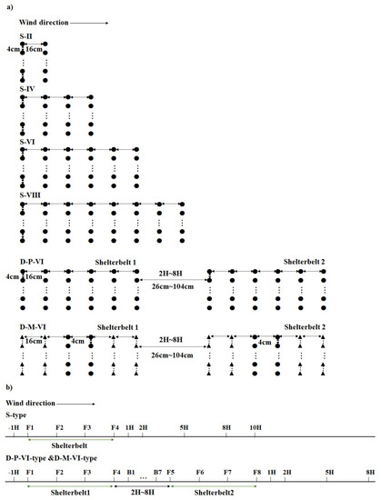
Figure 2.
Design of the shelterbelt model and distribution of the wind speed observation points. Sub-figure (a) shows the different configuration modes of the shelterbelt (● arbor; ▲ shrub). Sub-figure (b) shows the distribution of the wind speed observation points of three types of shelterbelts (S-type represents the single shelterbelt with different rows; D-P-VI-type represents double pure shelterbelts comprising arbors; D-M-VI-type represents double mixed shelterbelts comprising arbors and shrubs, and VI represents the number of rows in each shelterbelt; H represents the height of the arbor).
To ensure the accuracy and reliability of the test results, the experimental process must meet the requirements of “geometric similarity”, “kinematic similarity”, and “motion similarity” [48,49]. According to White [50] and Zhang et al. [51], the Reynolds number (Re) and Froude number (Fr) are the key dimensionless parameters to be considered in the wind tunnel experiments. The minimum Re chosen for this experiment was 6.1 × 10⁵ at a wind speed of 8 m·s−1. As the flow state can be considered fully turbulent when Re is >104, the experiment meets the self-simulation requirements. Under experimental conditions, the thickness of the boundary layer was >15 cm and the total height of the plant model was ≤13 cm. The wind speed profile in the boundary layer, i.e., the wind tunnel, met the logarithmic distribution consistent with nature and the thickness of the boundary layer was sufficient to meet the wind speed profile similarity condition. According to Zhang et al. [51], the Fr (Fr = v2 × (gH)−1) in the wind tunnel simulation experiment must be <20. The maximum wind speed in this experiment was 8 m·s−1 and the height of the wind tunnel was >0.73 m. Thus, the similarity criterion was met. Based on the geometric similarity theory [48] and a field survey of the vegetation height and diameter at breast height in the Green Ring Project, the ratio of the wind tunnel laboratory plant model to the field protective forest model was determined to be 1:25. The field survey results showed that the Green Ring Project forest belt configuration comprises six rows and multiple belts and the trees in the forest belt are arranged in a rectangular configuration with a plant spacing of 1 × 4 m. The tree species configuration mainly comprises a mixed forest of arbors and shrubs and pure tree forest. The belt spacing of the shelterbelt varies from 12 to 24 m, with a proportional reduction of 3.6H–7.3H. Based on the field conditions, the heights of the trees and shrubs were mainly 300 and 100 cm, respectively. Therefore, the experimental plant models were scaled to 13 and 4.5 cm to represent the heights of the arbor and shrubs, respectively. In this study, the maximum height of the plant model (13 cm) was 86.7% of the depth of the boundary layer in the wind tunnel (15 cm), which did not fully satisfy the requirement recommended by White [50]. Therefore, our study was not under full-scale conditions. However, according to White [50], if the Reynolds number exceeds a minimum critical value of approximately 104, the required ratio of >20% of the height of the plant model to the depth of the boundary layer in the wind tunnel and full-scale condition can be relaxed. Similar to Bhutto et al. [52], in this wind tunnel experiment, the Reynolds numbers for the three undisturbed velocities ranged from 8.92 × 10⁴ to 2.03 × 10⁵, which are large enough to meet the requirements of the Reynolds number independence regime recommended by White [50]. Therefore, this experiment met the requirements. Based on the experimental purpose and actual field conditions of the protection forest, four configuration models (S-II, S-IV, S-VI, and S-VIII; plant spacing was proportionally reduced to 4 × 16 cm) were designed for the wind tunnel simulation experiments. The configuration with the best number of rows was derived by analyzing the wind protection effectiveness of the four S-type protection forests. Based on the above results, seven D-P and D-M protection forest models with different belt spacings (ranging from 2H to 8H) were designed to compare and analyze their shelter efficiencies and determine the double shelterbelt configurations with the best wind protection capability. Figure 3 shows the dimensions of the plant model used in the wind tunnel experiment and the shelterbelt configurations.
2.2. Data Analysis
The shelter efficiency is an important indicator of the degree of airflow reduction by forest strips [49] and it can be expressed according to Equation (1):
where Exyz is the effectiveness of wind protection at the coordinates (x, y, z), %; Vijk is the average wind speed of the empty field, m·s−1; and Vxyz is the actual average wind speed measured in the shelterbelt at the same height, m·s−1.
Effective protection areas and effective protection ratios are often used to assess the shelter efficiency of protective forests. The effective protection area is the area protected when the protection forest has a specific shelter efficiency, which can be calculated from the shelter efficiency contour map using the grid volume tool in Surfer software. The effective protection ratio is the ratio of the area at or above a specific shelter efficiency to the total protection area (measurement area [53]) and can be measured by the p value (Equation (2)):
where P(m) is the cumulative effective protection ratio when the windproof efficiency is ≥m, %; Si is the effective protection area with a windproof efficiency interval of i, cm2; Emax is the highest value of windbreak efficiency behind the forest belt, %; and S0 is the total area of the protection area (measurement area), cm2.
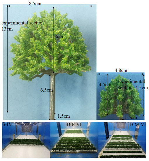
Figure 3.
Shelterbelt configurations (1.5 cm at the bottom of the trunk for fixing).
Kriging [54] is a regression algorithm for spatial modeling and predictive interpolation of random fields based on the covariance function, which can be used as a proxy model to interpolate limited simulation results to ensure local optimal data estimation in numerical experiments. Compared with traditional interpolation methods, such as least squares and distance-weighted average, kriging, which is a typical geostatistical algorithm, considers the spatially relevant properties of describing objects in the process of data gridding, making the interpolation results more scientific and closer to the actual situation. Therefore, kriging is widely used for the interpolation of observations of near-ground wind fields, air temperature and precipitation.
In this study, the Golden Software Surfer 16.0 was used for data visualization. The wind protection efficiency contour map was plotted based on actual measurements. The measurements were then interpolated using a Kriging interpolation.
3. Results
3.1. Analysis of the Shelter Efficiency of the Single Shelterbelt
3.1.1. Characteristics of the Wind Field of the Single Shelterbelt
The area with a shelter efficiency value above zero was determined to be the deceleration zone and that with a shelter efficiency value below zero was the acceleration zone. Furthermore, the larger the absolute value of shelter efficiency, the smaller the wind speed. Therefore, the contour map of the distribution of the shelter efficiency can also show the wind field distribution characteristics of the shelterbelt. Figure 4, Figure 5 and Figure 6 show that the distribution characteristics of the airflow fields of these four “single shelterbelts” with different numbers of rows are similar under the same wind speed and the difference lies in the influence range of each typical airflow field. Additionally, the distribution characteristics of the airflow fields around the shelterbelt of the same configuration are largely similar at different wind speeds and are distinguished by the range of influence of each typical airflow field. The characteristic zones of airflow fields around pure tree forest stands with different structures can be classified according to shelter efficiency as follows: (i) local acceleration region near the ground at the leading edge of the shelterbelt (A1); (ii) acceleration region above the shelterbelt (A2); (iii) deceleration region in front of the shelterbelt (B1); (iv) strong deceleration region in the canopy layer (B2); (v) weak deceleration region behind the shelterbelt (in the trunk layer at the trailing edge of the shelterbelt and the rear section of the shelterbelt at this height) (B3); and (vi) recovery region behind the shelterbelt (B4). Figure 4, Figure 5 and Figure 6 also show that, for a shelterbelt area, the shelter efficiency of the shelterbelt decreases as the target wind speed increases.
Figure 4, Figure 5 and Figure 6 show that a local acceleration region formed near the ground level at the leading edge of the upwind side in all four shelterbelt types (S-II, S-IV, S-VI, and S-VIII). The airflow was forced to divert and partially pass between the plant models, called narrow-tube airflow (i.e., through-flow), which increased the flow velocity of this airflow [55]. In all four shelterbelts, an acceleration region formed above the shelterbelt (above the height range of 2.5H) and extended over a wide area in the downwind direction. The areas with high wind speed are the smallest and largest in the S-II and S-VIII shelterbelts, respectively. This means that the region with the highest wind speed that forms above the shelterbelt increases with an increasing number of rows in a single shelterbelt. Figure 4, Figure 5 and Figure 6 also show that the shelter efficiency of the shelterbelt increases significantly when the airflow approaches the edge of the upwind side of the shelterbelt region [4], helping to form a deceleration region. The shelter efficiency is more notable at the height of the canopy layer of the shelterbelt. At this height, a strong deceleration region forms in the canopy layer of the shelterbelt and in a certain area behind the shelterbelt (~2.5H behind the shelterbelt). The works of Finnigan [56] and Belcher et al. [45], who observed that the leaf density is the largest and the void ratio is the smallest at the canopy height, confirm this point. The airflow might be affected by the low-velocity airflow in the shelterbelt canopy layer as the wind passes through the trunk of the shelterbelt and the wind speed decreases in the downwind distance and extends to a distance behind the shelterbelt region, helping to form a low-deceleration region. After airflow passes through the shelterbelt region, the wind speed continues to recover to the open-field wind speed along the downwind direction; this might be due to the acceleration of the airflow above the shelterbelt region (downward transfer of airflow momentum from above [4]), helping to form a recovery region behind the shelterbelt.
To further determine the correlations among belt spacing and shelter efficiency, the effective protection area behind the shelterbelt and the effective protection ratio between the shelterbelts under different belt spacings and shelter efficiencies were analyzed.
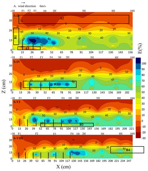
Figure 4.
Contour map of the distribution of the shelter efficiency of single shelterbelts with different rows. The abscissa represents the downwind distance (cm) and the ordinate represents the vertical height (cm). The top abscissa represents the observation point. 6 m·s−1. The legend indicates the shelter efficiency. In addition, “A1,A2; B1–B4” are, respectively, (i) local acceleration region near the ground at the leading edge of the shelterbelt (A1); (ii) acceleration region above the shelterbelt (A2); (iii) deceleration region in front of the shelterbelt (B1); (iv) strong deceleration region in the canopy layer (B2); (v) weak deceleration region behind the shelterbelt (in the trunk layer at the trailing edge of the shelterbelt and in the rear section of the shelterbelt at this height) (B3); and (vi) recovery region behind the shelterbelt (B4).
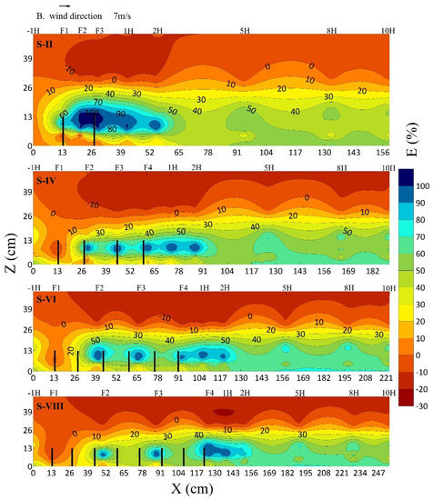
Figure 5.
Contour map of the distribution of the shelter efficiency of single shelterbelts with different rows. The abscissa represents the downwind distance (cm) and the ordinate represents the vertical height (cm). The top abscissa represents the observation point. 7 m·s−1. The legend indicates the shelter efficiency.
3.1.2. Effective Protection Area of the Single Shelterbelt
For a target wind speed of 7 m·s−1, Figure 7 shows that under the same wind speed and different shelter efficiencies, the effective protection area of the shelterbelt with different configurations significantly differs. In terms of wind protection capacity among these four types of single shelterbelt with different numbers of rows, the S-II type had the lowest shelter efficiency, whereas the S-VI type had the highest shelter efficiency which approached that of the S-VIII-type. The shelter efficiency of single shelterbelts (S-type) increased with the number of plant rows. However, because the number of plant rows is not the only factor governing the shelter efficiency of the shelterbelts, the shelter efficiency and the number of plant rows did not show a positive correlation. The effective protection area after the shelterbelt decreased with increasing shelter efficiency. When the efficiency of the shelter was large, the shelterbelt almost lost its wind-prevention ability. Figure 7 shows that when the shelter efficiency is higher than 70%, the effective protection area behind the shelterbelt decreases sharply. For example, in the range of 0H–10H behind the shelterbelt and a vertical height of 0H–3H, when the shelter efficiency of the shelterbelt increased from 60% to 70%, the effective protection area of the S-VI-type shelterbelt decreased sharply from 1643 to 436 cm2. Additionally, comparing the contour map distribution of shelter efficiency at three wind speeds in Figure 4, Figure 5 and Figure 6, the effective protection area behind the shelterbelt in the same area with the same configuration mode decreases continuously with increasing wind speed; therefore, it can be inferred that the shelterbelts lose their wind protection capacity when the wind speed is high.
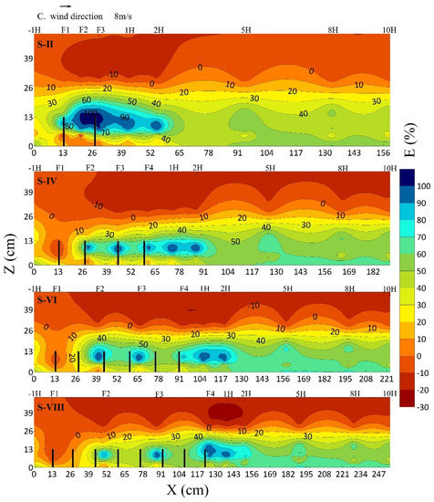
Figure 6.
Contour map of the distribution of the shelter efficiency of single shelterbelts with different rows. The abscissa represents the downwind distance (cm) and the ordinate represents the vertical height (cm). The top abscissa represents the observation point. 8 m·s−1. The legend indicates the shelter efficiency.
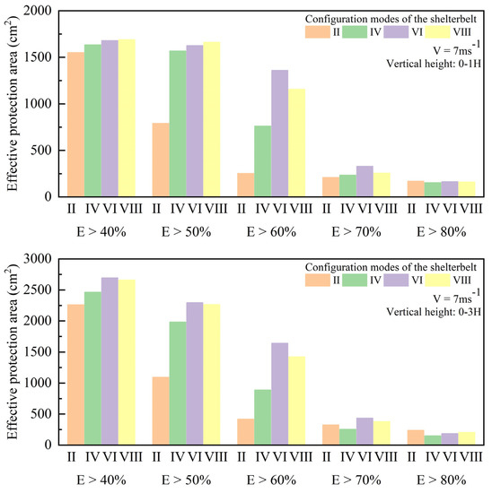
Figure 7.
Effective protection area in the range of 0–10H behind the single shelterbelt. The abscissa represents the shelterbelt configuration under the specific shelter efficiency and the ordinate represents the effective protection area (cm2). (V) 7 m·s−1.
3.2. Analysis of Shelter Efficiency of the Double Shelterbelts
3.2.1. Wind Field Characteristics of the Double Shelterbelts
The distribution characteristics of the airflow fields around the D-P-VI protective forest with the same belt spacing are similar under three wind speeds (6, 7, and 8 m·s−1). The experimental results at 7 m·s−1 served as an example to analyze the airflow characteristics around the D-P-VI protective forest with different belt spacings. Figure 8 shows that the distribution characteristics of the airflow fields around the seven D-P-VI-type protective forests with different belt spacings (2H–8H) are similar at the same wind speed. In contrast to the single pure arbor shelterbelt (Figure 4, Figure 5 and Figure 6), there was no local acceleration region near the ground at the leading edge of the second shelterbelt (far from the wind source) and the deceleration region at the height of the trunk layer at the rear edge of the first forest belt did not extend to the front edge of the second shelterbelt. This may be due to the effect of airflow from the strong deceleration region at the height of the upper canopy, based on which the wind speed decreases with the downwind distance. The strong deceleration region extended over a long range between the two shelterbelts. At a belt spacing of 2H–6H, the canopy height in the shelterbelt belonged to a strong deceleration zone. At belt spacings of 7H and 8H, the canopy height range of the front edge of the second shelterbelt did not belong to the strong deceleration region. In addition, there was no weak deceleration zone in the trunk layer at the trailing edge of the second shelterbelt and in the rear section of the shelterbelt, which may be due to the significant reduction in the kinetic energy of the airflow after it passes through the first shelterbelt. The wind speed decreased significantly when it reached the second shelterbelt.
The distribution characteristics of the airflow fields around the D-M-VI protective forest with the same belt spacing were similar under the three wind speeds (6, 7, and 8 m·s−1). The experimental results (Figure 9) at 7 m·s−1 were used as an example to analyze the airflow characteristics around the D-M-VI protective forest with different belt spacings. In contrast to the D-P-VI shelterbelt, there was no local acceleration zone near the ground at the front edge of the two shelterbelts in the D-M-VI shelterbelt, which may be due to the height of the shrubs in the shelterbelt, which was almost the same as that of the tree trunk layer, leading to a small porosity of the shelterbelt and thus greatly hindering the airflow from passing through the trunk layer. Most of the airflow passes above the shelterbelt canopy as overflow. Therefore, in contrast to the S-type and D-P-VI shelterbelts, a weak deceleration region (B3) did not form in the D-M-VI shelterbelt and the coverage of the strong deceleration region (B2) was much larger than the D-P-VI shelterbelt. Figure 9 shows that the distribution area of B2 extended from the tree canopy of the first shelterbelt to a distance behind the second shelterbelt. However, with the increase in the belt spacing, the area of the second half between the two shelterbelts and the first half of the second belt became a weak deceleration region. At belt spacings of 5H and 6H, the area of the first half of the second shelterbelt was a weak deceleration region. At belt spacings of 7H and 8H, the area of the second half between the two shelterbelts and the first half of the second belt was a weak deceleration zone.
3.2.2. Effective Protection Area of the Double Shelterbelts (behind “Shelterbelt 2”)
Figure 10 shows that the effective protection area behind the shelterbelt of the same protection forest did not vary significantly under the same shelter efficiency and the same belt spacing, especially for the D-M-VI shelterbelt. For example, when the shelter efficiency was 50%, the effective protection area behind the D-M-VI shelterbelt ranged from 1313 to 1557 cm2 at the seven different belts spacing, and when the shelter efficiency was 60%, the effective protection area varied from 695 to 836 cm2. For the D-P-VI-type protective forest, the effective protection area behind the shelterbelt showed a decreasing trend when the belt spacing was increased under the same shelter efficiency. When the belt spacing was 7H, the effective protection area behind the shelterbelt was the smallest. Comparing the effective protection area behind the shelterbelt of the two protective forests (D-P-VI and D-M-VI), in the range of 0H–8H behind the shelterbelt and at a vertical height of 0H–3H, the wind protection ability of the D-P-VI-type protective forest was superior to that of the D-M-VI-type protective forest with the same shelter efficiency and belt spacing. For example, when the shelter efficiency was 50%, the effective protection area behind the D-P-VI-type protective forest varied from 1803 to 2059 cm2, whereas the effective protection area behind the D-M-VI-type protective forest varied from 1313 to 1557 cm2. When the shelter efficiency was 60%, the former varied from 1071 to 1651 cm2, and the latter from 695 to 836 cm2.
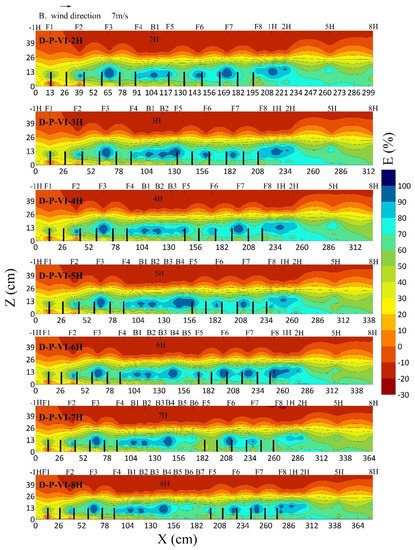
Figure 8.
Contour map of the distribution of the shelter efficiency of double pure arbor shelterbelts under different belt spacings. The belt spacing ranges from 2H to 8H. The abscissa represents the downwind distance (cm) and the ordinate represents the vertical height (cm). The top abscissa represents the observation point. 7 m·s−1. The legend indicates the shelter efficiency.
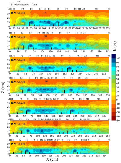
Figure 9.
Contour map of the distribution of the shelter efficiency of double mixed shelterbelts of arbors and shrubs under different belt spacings. The belt spacing ranges from 2H to 8H. The abscissa represents the downwind distance (cm) and the ordinate represents the vertical height (cm). The top abscissa represents the observation point. The legend indicates the shelter efficiency.
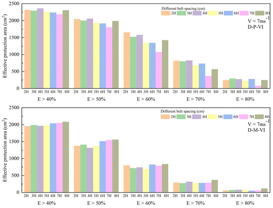
Figure 10.
Effective protection area of double shelterbelts in the range of 0H–8H behind the shelterbelt at a vertical height of 0H–3H. The abscissa represents the shelterbelt with different belt spacings under a certain shelter efficiency. For example, “6H–50%” indicates a protection forest with a shelter efficiency of ≥50% and belt spacing of 6H. The ordinate represents the effective protection area (cm2).
3.2.3. Effective Protection Ratio of Double Shelterbelts (between the Shelterbelts)
Comparing the effective protection ratio between the shelterbelts of the D-P-VI and D-M-VI protective forests, it can be concluded that the wind protection ability of the D-M-VI protective forest was superior to that of the D-P-VI protective forest under the same shelter efficiency and belt spacing (Figure 11). Figure 11 shows that the effective protection ratio between the shelterbelts of the D-P-VI protective forest with different belt spacings varied little under the same shelter efficiency and the difference between shelterbelts of the D-M-VI protective forest was even smaller. For example, when the shelter efficiency was 50%, the effective protection ratio between shelterbelts of the D-P-VI protective forest varied from 41.89% to 49.74%, whereas that of the D-M-VI protective forest varied from 56.22% to 57.11%. When the shelter efficiency was 60%, the range of variation was 33.42–41.01% for the D-P-VI protective forest compared to 50.69–53.03% for the D-M-VI protective forest. For the D-M-VI protective forest, the effective protection ratio between the strips of the protection forest showed a decreasing trend with the increase in the belt spacing under the same shelter efficiency. However, the D-M-VI protective forest maintained a good protection effect when the belt spacing was increased to 8H. For example, when the shelter efficiency was 70%, 40.08% of the area between the shelterbelts can reach over 70%.
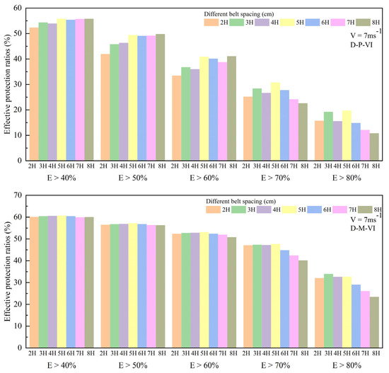
Figure 11.
Effective protection ratio between double shelterbelts with different belt spacings at a vertical height of 0H–3H. The abscissa represents the shelterbelt with different belt spacings under a certain shelter efficiency. For example, “6H–50%” indicates a protection forest with a shelter efficiency of ≥50% and belt spacing of 6H. The belt spacing ranges from 2H to 8H.
4. Discussion
Based on the analysis of the contour map of the shelter efficiency of single shelterbelts with different numbers of rows (Figure 4, Figure 5 and Figure 6), it can be concluded that only the part of the airflow that reaches the shelterbelt can cross over it to merge with the upper flow due to the blockage of the shelterbelt canopy and a small part is weakened by friction with the upper airflow during lifting. Therefore, the wind speed decreases in a certain area above the shelterbelt canopy but an acceleration region forms in the area away from the forest canopy (i.e., the airflow convergence area in which the wind speed increases [57]). The kinetic energy of the other part of the airflow that passes through the interior of the shelterbelt is significantly weakened by the disturbance and friction provided by branches, leaves, and trunks [58,59]. However, a local acceleration region forms near the ground at the front edge of the shelterbelt region due to the narrow-tube effect [55,60]. Baldocchi et al. [61] and Hesp et al. [62] also showed that accelerated airflow near the ground can be observed in the lower part of plant stands, especially for canopies characterized by an open space between plants. These two processes cause the wind speed to decrease significantly within a certain range before and after the shelterbelt [63]. Thus, the airflow is significantly reduced when it reaches the shelterbelt, forming a deceleration region in front of the shelterbelt. The kinetic energy of airflow is reduced in a fluctuating manner due to discontinuous (i.e., with certain row spacing) blockage by plants in the shelterbelt and it reaches a minimum after the shelterbelt [4]. However, the effect on the wind speed varies behind and in front the shelterbelt region because of the different configurations of the shelterbelt and the formation of different airflow field structures. The wind speed significantly decreases at the shelterbelt edge behind and in front of the shelterbelt but recovers rapidly with increasing distance behind the shelterbelt [58]. The results are consistent with wind tunnel simulations of the shelter efficiency of protective forests by Ma et al. [4] and Zhang et al. [64].
Comparing the spatial distribution of the shelter efficiency of shelterbelts with different configurations under three wind speeds (Figure 5, Figure 8 and Figure 9), it was found that several characteristic areas of the airflow field were generated around the shelterbelt by the blocking effect of the protective forest, independent of the target wind speed. These results are consistent with those of Mayaud et al. [44] and Torshizi et al. [65] regarding wind tunnel simulations and field observations. The magnitude of the wind speed only affected the extent of the acceleration and deceleration regions, which is consistent with reports of Ma et al. [4] regarding the airflow field around the shelterbelt. Based on shelter efficiency [66], the airflow field around the single shelterbelt (Figure 4, Figure 5 and Figure 6) can be divided into six characteristic regions: (i) local acceleration region near the ground at the leading edge of the shelterbelt (A1); (ii) acceleration region above the shelterbelt (A2); (iii) deceleration region in front of the shelterbelt (B1); (iv) strong deceleration region in the canopy layer (B2); (v) weak deceleration region behind the shelterbelt (in the trunk layer at the trailing edge of the shelterbelt and the rear section of the shelterbelt) (B3); and (vi) recovery region behind the shelterbelt (B4). Unlike the single shelterbelt (S-type), for “Double shelterbelts”, the wind speed decreased with the downwind distance, probably due to the influence of airflow from the strong deceleration region at the height of the shelterbelt canopy above. Therefore, the kinetic energy of airflow in the D-P-VI; shelterbelt (Figure 8) was too small when it reached the second shelterbelt and there was no local acceleration region near the ground at the shelterbelt edge. Because the height of the shrubs in the D-M-VI-type shelterbelt (Figure 9) was almost the same as that of the tree trunk layer, the porosity of the protective forest was particularly small, which greatly hindered the airflow from the trunk layer to pass and most of the airflow passed over the forest canopy as overflow. Therefore, no local acceleration region was generated near the ground at the front edge of both shelterbelts in the D-M-VI protective forest and no weak deceleration region (B3) was generated at the height of the tree trunk layer in the latter half of the protective forest and the rear section of the shelterbelt. Comparing the shelter efficiency of protective forests with the same configuration under three sets of wind speeds shows that the higher the target wind speed in the same area of the shelterbelt, the smaller the reduction in the wind speed by the protection forest [4] and the lower its shelter efficiency. Therefore, it can be predicted that the protective forest loses its wind protection effect when the wind speed is too high.
The effective protection area, the area protected when the protection forest has a specific shelter efficiency, and effective protection ratio, the ratio of the area at or above a specific shelter efficiency to the total protection area (measurement area [53]), are often used to assess the shelter efficiency of protective forests. Based on a comparison of the effective protection area or effective protection ratio under specific shelter efficiencies, the differences in the shelter efficiencies of protection forests under different configurations can be more accurately determined, which provides a theoretical basis for the comparison of the protection areas of protected forests. Our results regarding the wind protection ability of a single pure arbor shelterbelt showed that the shelter efficiency of the S-VI-type shelterbelt was significantly higher than those of the S-II, S-IV, and S-VIII shelterbelts because the effective protection distance of this protection forest increases with an increasing number of rows in the shelterbelt because the windbreak effect is not lost [5,12,18,29]. However, there is no linear relationship between the wind protection effectiveness and number of rows [30]. When some rows are planted, the main factor that affects the effective protection distance of a shelterbelt is the height of the shelterbelt [18,67,68]. Furthermore, from the viewpoint of plant water consumption, the S-VI shelterbelt is a better choice than the S-VIII shelterbelt. The wind protection ability of the D-P-VI (the double pure shelterbelts) and D-M-VI shelterbelts (double mixed shelterbelts) can be ordered as D-P-VI > D-M-VI in the range of 0H–8H behind the protected forest stand and below 3H height from the ground. However, it is D-M-VI > D-P-VI in the height range of 3H from the ground between the protected forest stands. Under the same belt spacing, the shelter efficiency behind the shelterbelt of the D-P-VI protection forest was better than the D-M-VI protection forest but the shelter efficiency between shelterbelts of the D-M-VI protection forest was better than that of the D-P-VI protection forest because the overall height of the D-P-VI protective forest was larger than that of the D-M-VI protective forest. This extends the effective protection distance of the protective forest. The height of shrubs in the D-M-VI protective forest was almost the same as that of the tree trunk layer, which significantly hinders the passage of airflow, making the wind speed between the D-M-VI protective forest smaller than that between the D-P-VI protective forest.
Based on the comparison of the shelter efficiency of the D-P-VI and D-M-VI protective forests with the same belt spacing, the differences in the overall wind protection capacity were insignificant, although there were differences in the shelter efficiency between the two configurations of protective forests. The advantage of the D-P-VI protective forests is that they can provide a larger area of protection when the wind protection needs of the protected objects are low. In contrast, D-M-VI is a better choice when the wind protection needs of the target are greater. In terms of shelter efficiency near the ground, the shelter efficiency of the D-M-VI-type shelterbelt is higher than the D-P-VI-type shelterbelt in the same area. In addition, the D-M-VI shelterbelt may provide more significant ecological benefits than the D-P-VI shelterbelt [68]. For example, D-M-VI shelterbelts can improve (i) the efficiency of light energy use, (ii) the microclimate of the region, (iii) the resistance of plants to pests and diseases, and (iv) biodiversity [69,70,71]. The water consumption capacity of the D-P-VI protective forest is higher than the D-M-VI protective forest, which must be considered when selecting the configuration of a protective forest in a water-scarce area. Furthermore, a single-species D-P-VI shelterbelt may be more susceptible to pests and diseases. Therefore, if a shelterbelt is needed to provide a larger area of protection, it should be constructed using a combination of arbors of different tree species.
In addition, because Nursultan belongs to a typical temperate continental climate zone, the winters are cold and long and many snowstorms occur. During the long winter season, the protective forest acts as a snowbreak, which can reduce the amount of flying snow and snow accumulation in a certain area around the protective forest by decreasing the intensity of wind and snow flow [72], which has good ecological benefits. The results of a previous study showed that snow accumulation is predominant on the upwind side if the snowbreak forest is high; if the snowbreak is low, snow accumulation often occurs within the forest or on the downwind side of the forest [71]. However, the snow protection capacity of a protective forest is not only dependent on the height of the shelterbelt as the structure of the shelterbelt can directly affect its snow retention capacity [73]. In addition, protective forests not only retain large amounts of snow but also prolong snowmelt, regulate snowmelt runoff, and extend the snowmelt period. Based on the characteristics of snowbreak forests, the D-P-VI shelterbelt is better than the D-M-VI shelterbelt in terms of the snow protection capacity. However, in terms of snow retention capacity, the D-M-VI protective forest is better. The mixed shelterbelt can retain a large amount of snow within and between the shelterbelts which can effectively prolong the snowmelt period and provide better soil moisture for the growth of the following year’s vegetation. Based on the analysis and comparison of the shelter efficiencies of shelterbelts under different belt spacings, the difference in the shelter efficiency of shelterbelts with the same configuration mode was insignificant when the belt spacing was 2H–8H. However, considering the snow-prevention ability of the protective forest, the greater the belt spacing, the better the protection of the snowbreak given, so that the protective forest has high wind and snow-prevention benefits.
Based on field survey data, we provide the following suggestions for the construction of plantation forests’ Green Ring Project considering the climate and site conditions of Nursultan, species diversity, forest water balance, and positive effect of the configuration of the spatial structure of shelterbelts on wind protection benefits and the prevention of wind and snow disasters combined with the existing configuration of the shelterbelt: (i) In areas in which seedlings or other low crops must be cultivated, it is suitable to build D-M-VI-type protective forests because of their relatively high wind protection needs and this planting can provide relatively static winds for the protection objects. (ii) In areas close to traffic arteries, it is suitable to build double mixed shelterbelts of arbors and shrubs planting configurations with six belt rows, four rows of arbors, and two rows of shrubs in which arbors are planted close to the downwind side and shrubs are planted close to the upwind side. This planting mode (D-M-II-IV shelterbelt) provides better wind protection benefits and better snow protection benefits in winter. It improves road visibility and traffic safety. (iii) In areas around settlements, it is suitable to build D-P-VI shelterbelts with arbors of different species. This planting mode provides a larger area of protection and most of the snow remains on the upwind side of the protective forests in winter. (iv) Considering the effective protection distance of the shelterbelt, it is necessary to increase the construction of protective forests in the inner part of the city and windward area of the main wind direction in winter (northeastern part of the city) to effectively reduce the effect of snowstorms on the city of Nursultan. This can expand the effective protection range of the protective forests and better protect the city.
5. Conclusions
In this study, the shelter efficiencies and effective protection areas of protective forests under different shelterbelt configurations were studied. These conclusions can be drawn:
- There are similarities and differences among the three types of protective forests in the S, D-P-VI, and D-M-VI shelterbelt configurations. The distributions of their airflow fields are similar and can be divided into the pre-forest deceleration region, acceleration region above the shelterbelt, strong canopy deceleration region, post-forest deceleration region, and post-forest recovery region. The difference between them is that the typical airflow field around each type of protection forest has a different distribution area and influence range, which greatly affects the effective protection range.
- In the existing shelterbelt configuration of Nursultan, the wind protection capacity of the S-type protective forest can be ordered as S-VI > S-VIII > S-IV > S-II. The wind protection capacity behind the double shelterbelts has the following order: D-P-VI > D-M-VI. The wind protection capacity between the double shelterbelt can be ordered as D-M-VI > D-P-VI. In terms of the shelter efficiency near the ground, the shelter efficiency of the D-M-VI-type shelterbelt is higher than that of the D-P-VI-type shelterbelt, given the same area. Under the same belt spacing, the shelter efficiency of the D-P-VI shelterbelt behind the shelterbelt is better than the D-M-VI shelterbelt, but the shelter efficiency of the D-M-VI shelterbelt between the two shelterbelts is better than that of the D-P-VI shelterbelt.
- D-M-V-type shelterbelts are suitable to be built in areas where seedlings or other low plants must be cultivated; D-M-II-IV shelterbelts are suitable for construction around the traffic trunk line. Around residential areas, D-P-VI shelterbelts are more suitable. Moreover, although the windbreak benefits of shelterbelts with the same configuration but different belt spacings (2H–8H) differ insignificantly, the greater the belt spacing, the higher the ecological benefit within a certain range, especially the snow-prevention benefit. Furthermore, to effectively reduce the effects of snowstorms and other natural disasters on Nursultan, shelterbelts should be constructed in the upwind direction (northeast) of the dominant wind direction in winter in the city.
Author Contributions
Conceptualization, H.L., Y.W., S.L., A.A. and H.W.; Data curation, H.L., A.A. and H.W.; Formal analysis, H.L.; Funding acquisition, Y.W.; Methodology, H.L., Y.W. and S.L.; Resources, S.L.; Software, H.L., A.A. and H.W.; Writing—original draft, H.L.; Writing—review and editing, Y.W., S.L., A.A. and H.W. All authors have read and agreed to the published version of the manuscript.
Funding
This study was supported by the Strategic Priority Research Program of the Chinese Academy of Sciences (No. XDA20030102) and the CAS Key Technology Talent Program (Study on the technology of desertification in the Belt and Road).
Institutional Review Board Statement
Not applicable.
Informed Consent Statement
Not applicable.
Data Availability Statement
Experimental data are available from the corresponding author upon reasonable request.
Conflicts of Interest
The authors declare no conflict of interest.
References
- Rosenberg, N.J. Microclimate: The Biological Environment; Wiley: New York, NY, USA, 1974. [Google Scholar]
- Cornelis, W.; Gabriels, D. Optimal windbreak design for wind-erosion control. J. Arid Environ. 2005, 61, 315–332. [Google Scholar] [CrossRef]
- Guan, D. Aerodynamic Effects of Farmland Windbreak System. D; Institute of Applied Ecology, Chinese Academy of Sciences: Beijing, China, 1998. [Google Scholar]
- Ma, R.; Li, J.; Ma, Y.; Shan, L.; Li, X.; Wei, L. A wind tunnel study of the airflow field and shelter efficiency of mixed windbreaks. Aeolian Res. 2019, 41, 100544. [Google Scholar] [CrossRef]
- Gao, H.; Wu, B.; Zhang, Y.Q.; Ding, G.D. Wind Tunnel Test of Wind Speed Reduction of Caragana Korshinskii Coppice. J. Soil Water Conserv. 2010, 24, 44–47. [Google Scholar]
- Liang, H.R.; Wang, J.Y.; Dong, H.R.; Yang, W.B.; Lu, Q.; Zhao, A.G. Wind Velocity Field and Windbreak Effects in Two Types of Low Density and Belt-Scheme Sand-Break Forests. J. Ecol. 2010, 30, 568–578. [Google Scholar]
- Zhou, Q.Z.; Zhao, Y.; Gao, G.L.; Zhang, Y.; Cheng, Y.X. Wind Tunnel Simulation Experiment of Windbreak Effects of Shelterbelt Along Xining-Golmud Section of Qinghai-Tibet Railway. Ningxia Agric. For. Sci. Technol. 2018, 59, 4. [Google Scholar]
- Xu, L.S.; Mu, G.J.; Sun, L.; Ren, X.; Zhou, J. Effect of Shelterbelt on Dust Deposition at Surface Layer: A case study in Cele, Xinjiang, China. J. Desert Res. 2017, 37, 57–64. [Google Scholar]
- Zhou, Y.H.; Chen, Z.; Tong, X.; Zhuo, C.X.; Liu, H.Y.; Hao, B.E. The Windproof Effect of Caragana korshinskii with Different Porosity. J. Soil Water Conserv. China 2022, 5, 60–64. [Google Scholar]
- Li, X.Y.; Wang, K.J.; Gu, J.C.; Liu, Q.G.; C, Y. Windbreak Effect Model of Forest Belts with Different Structure. J. Desert Res. 2019, 39, 118–125. [Google Scholar]
- Tang, Y.L.; An, Z.S.; Zhang, K.C.; Tan, L.H. Wind Tunnel Simulation of Windbreak Effect of Single-row Shelter Belts of Different Structure. J. Desert Res. 2012, 32, 647–654. [Google Scholar]
- Cheng, H.; Liu, C.; Kang, L. Experimental study on the effect of plant spacing, number of rows and arrangement on the airflow field of forest belt in a wind tunnel. J. Arid Environ. 2020, 178, 104169. [Google Scholar] [CrossRef]
- Musick, H.B.; Gillette, D.A. Field evaluation of relationships between a vegetation structural parameter and sheltering against wind erosion. Land Degrad. Dev. 1990, 2, 87–94. [Google Scholar] [CrossRef]
- Cheng, H.; He, W.; Liu, C.; Zou, X.; Kang, L.; Chen, T.; Zhang, K. Transition model for airflow fields from single plants to multiple plants. Agric. For. Meteorol. 2018, 266–267, 29–42. [Google Scholar] [CrossRef]
- Wolfe, S.; Nickling, W.G. The protective role of sparse vegetation in wind erosion. Prog. Phys. Geogr. Earth Environ. 1993, 17, 50–68. [Google Scholar] [CrossRef]
- Cheng, H.; Zhang, K.; Liu, C.; Zou, X.; Kang, L.; Chen, T.; He, W.; Fang, Y. Wind tunnel study of airflow recovery on the lee side of single plants. Agric. For. Meteorol. 2018, 263, 362–372. [Google Scholar] [CrossRef]
- Gillies, J.A.; Lancaster, N.; Nickling, W.G.; Crawley, D.M. Field determination of drag forces and shear stress partitioning effects for a desert shrub (Sarcobatus vermiculatus, greasewood). J. Geophys. Res. Earth Surf. 2000, 105, 24871–24880. [Google Scholar] [CrossRef]
- Wu, T.; Yu, M.; Wang, G.; Wang, Z.; Duan, X.; Dong, Y.; Cheng, X. Effects of stand structure on wind speed reduction in a Metasequoia glyptostroboides shelterbelt. Agrofor. Syst. 2012, 87, 251–257. [Google Scholar] [CrossRef]
- Plate, E.J. The aerodynamics of shelter belts. Agric. Meteorol. 1971, 8, 203–222. [Google Scholar] [CrossRef]
- Raine, J.; Stevenson, D. Wind protection by model fences in a simulated atmospheric boundary layer. J. Wind Eng. Ind. Aerodyn. 1977, 2, 159–180. [Google Scholar] [CrossRef]
- Bitog, J.P.; Lee, I.-B.; Hwang, H.-S.; Shin, M.-H.; Hong, S.-W.; Seo, I.-H.; Kwon, K.-S.; Mostafa, E.; Pang, Z. Numerical simulation study of a tree windbreak. Biosyst. Eng. 2012, 111, 40–48. [Google Scholar] [CrossRef]
- Dong, Z.; Luo, W.; Qian, G.; Wang, H. A wind tunnel simulation of the mean velocity fields behind upright porous fences. Agric. For. Meteorol. 2007, 146, 82–93. [Google Scholar] [CrossRef]
- Gao, H. Study on the Windbreak and Barrier Band Effect of the Low Profile Afforestation. Ph.D. Thesis, Beijing Forestry University, Beijing, China, 2010. [Google Scholar]
- Grant, P.F.; Nickling, W.G. Direct field measurement of wind drag on vegetation for application to windbreak design and modelling. Land Degrad. Dev. 1998, 9, 57–66. [Google Scholar] [CrossRef]
- Lee, S.-J.; Park, K.-C.; Park, C.-W. Wind tunnel observations about the shelter effect of porous fences on the sand particle movements. Atmos. Environ. 2002, 36, 1453–1463. [Google Scholar] [CrossRef]
- Minvielle, F.; Marticorena, B.; Gillette, D.; Lawson, R.; Thompson, R.; Bergametti, G. Relationship between the Aerodynamic Roughness Length and the Roughness Density in Cases of Low Roughness Density. Environ. Fluid Mech. 2003, 3, 249–267. [Google Scholar] [CrossRef]
- Brandle, J.R.; Hodges, L.; Zhou, X.H. Windbreaks in North American agricultural systems. Agrofor. Syst. 2004, 65–78. [Google Scholar] [CrossRef] [Green Version]
- Yang, W.B.; Li, W.; Dang, H.Z. Low Coverage of Sand Control: Principles, Patterns and Effects; Science Press: Beijing, China, 2016. [Google Scholar]
- Cui, Q.; Feng, Z.S.; Pfiz, M.; Veste, M.; Kuppers, M.; He, K.N.; Gao, J.R. Trade-Off Between Shrub Plantation and Wind-Breaking in the Arid Sandy Lands of Ningxia, China. Pak. J. Bot. 2012, 44, 1639–1649. [Google Scholar]
- Liu, C.; Zheng, Z.; Cheng, H.; Zou, X. Airflow around single and multiple plants. Agric. For. Meteorol. 2018, 252, 27–38. [Google Scholar] [CrossRef]
- Marshall, J. Drag measurements in roughness arrays of varying density and distribution. Agric. Meteorol. 1971, 8, 269–292. [Google Scholar] [CrossRef]
- Liu, J.; Kimura, R.; Miyawaki, M.; Kinugasa, T. Effects of plants with different shapes and coverage on the blown-sand flux and roughness length examined by wind tunnel experiments. CATENA 2020, 197, 104976. [Google Scholar] [CrossRef]
- Miri, A.; Dragovich, D.; Dong, Z. The response of live plants to airflow—Implication for reducing erosion. Aeolian Res. 2018, 33, 93–105. [Google Scholar] [CrossRef]
- Woodruff, N.P.; Zingg, A.W. Wind Tunnel Studies of Shelterbelt Models. J. For. 1953, 51, 173–178. [Google Scholar]
- Wu, X.; Zou, X.; Zhou, N.; Zhang, C.; Shi, S. Deceleration efficiencies of shrub windbreaks in a wind tunnel. Aeolian Res. 2015, 16, 11–23. [Google Scholar] [CrossRef]
- Van Thuyet, D.; Van Do, T.; Sato, T.; Hung, T.T. Effects of species and shelterbelt structure on wind speed reduction in shelter. Agrofor. Syst. 2014, 88, 237–244. [Google Scholar] [CrossRef]
- Judd, M.J.; Raupach, M.R.; Finnigan, J.J. A wind tunnel study of turbulent flow around single and multiple windbreaks, part I: Velocity fields. Bound.-Layer Meteorol. 1996, 80, 127–165. [Google Scholar] [CrossRef]
- Leenders, J.K.; van Boxel, J.H.; Sterk, G. The effect of single vegetation elements on wind speed and sediment transport in the Sahelian zone of Burkina Faso. Earth Surf. Process. Landf. 2007, 32, 1454–1474. [Google Scholar] [CrossRef]
- Ash, J.E.; Wasson, R.J. Vegetation and Sand Mobility in the Australian Desert Dunefield. Z. Geomorphol. 1983, 45, 7–25. [Google Scholar]
- Leenders, J.K.; Sterk, G.; Van Boxel, J.H. Modelling wind-blown sediment transport around single vegetation elements. Earth Surf. Process. Landf. 2011, 36, 1218–1229. [Google Scholar] [CrossRef]
- Mayaud, J.R.; Wiggs, G.F.; Bailey, R.M. Characterizing turbulent wind flow around dryland vegetation. Earth Surf. Process. Landf. 2016, 41, 1421–1436. [Google Scholar] [CrossRef] [Green Version]
- Mayaud, J.R.; Wiggs, G.F.; Bailey, R.M. Dynamics of skimming flow in the wake of a vegetation patch. Aeolian Res. 2016, 22, 141–151. [Google Scholar] [CrossRef] [Green Version]
- Fu, L.-T.; Fan, Q.; Huang, Z.-L. Wind speed acceleration around a single low solid roughness in atmospheric boundary layer. Sci. Rep. 2019, 9, 12002. [Google Scholar] [CrossRef]
- Miri, A.; Davidson-Arnott, R. The effectiveness of a single Tamarix tree in reducing aeolian erosion in an arid region. Agric. For. Meteorol. 2021, 300, 108324. [Google Scholar] [CrossRef]
- Belcher, S.E.; Jerram, N.; Hunt, J.C.R. Adjustment of a turbulent boundary layer to a canopy of roughness elements. J. Fluid Mech. 2003, 488, 369–398. [Google Scholar] [CrossRef] [Green Version]
- A Kabanova, S.; Zenkova, Z.N.; A Danchenko, M. Regional risks of artificial forestation in the steppe zone of Kazakhstan (case study of the green belt of Astana). IOP Conf. Ser. Earth Environ. Sci. 2018, 211. [Google Scholar] [CrossRef]
- Zheng, Z.H.; Lei, J.Q.; Li, S.Y.; Wang, H.F.; Fan, J.L. Test and Evaluation of Wind Flow Characteristics of a Portable Wind Tunnel. J. Desert Res. 2012, 32, 1551–1558. [Google Scholar]
- Wu, Z. Geomorphology of Wind-Drift Sands and Their Controlled Engineering; Science Press: Beijing, China, 2003; pp. 332–403. (In Chinese) [Google Scholar]
- Ding, G. Wind Sand Physics, 2nd ed.; China Forestry Press: Beijing, China, 2010. [Google Scholar]
- White, B.R. Laboratory Simulation of Aeolian Sand Transport and Physical Modeling of Flow Around Dunes. Ann. Arid Zone 1996, 35, 187–213. [Google Scholar]
- Zhang, W.; Kang, J.-H.; Lee, S.-J. Tracking of saltating sand trajectories over a flat surface embedded in an atmospheric boundary layer. Geomorphology 2007, 86, 320–331. [Google Scholar] [CrossRef]
- Latif Bhutto, S.; Miri, A.; Zhang, Y.; Danish, A.B.; Cao, Q.Q.; Xin, Z.M.; Xiao, H.J. Experimental Study on the Effect of Four Single Shrubs on Aeolian Erosion in a Wind Tunnel. CATENA 2022, 212, 106097. [Google Scholar] [CrossRef]
- Bao, Y. Windbreak Effects of Shelterbelt in Oases Based on Wind Velocity Flow Field. Ph.D. Thesis, Beijing Forestry University, Beijing, China, 2015. [Google Scholar]
- Le, N.D.; Zidek, J.V. Statistical Analysis of Environmental Space-Time Processes; Springer: New York, NY, USA, 2006. [Google Scholar] [CrossRef]
- Vigiak, O.; Sterk, G.; Warren, A.; Hagen, L.J. Spatial modeling of wind speed around windbreaks. CATENA 2003, 52, 273–288. [Google Scholar] [CrossRef]
- Finnigan, J. Turbulence in Plant Canopies. Annu. Rev. Fluid Mech. 2000, 32, 519–571. [Google Scholar] [CrossRef]
- Ma, R.; Wang, J.; Qu, J.; Liu, H. Effectiveness of shelterbelt with a non-uniform density distribution. J. Wind Eng. Ind. Aerodyn. 2010, 98, 767–771. [Google Scholar] [CrossRef]
- Dong, Z. Research on Farmland Wind-Sand Disaster of Oasis and Its Control Mechanism in Ulan Buh Desert. Ph.D. Thesis, Beijing Forestry University, Beijing, China, 2004. [Google Scholar]
- Yang, T.T.; Chai, H.Q.; Yao, G.Z.; Ding, G.D. Study on Wind Breaking and Sand Blocking Effects of Farmland Shelterbelts in Ulan Buh Desert Oasis. For. Resour. Manag. 2006, 6, 42–45. [Google Scholar]
- Qu, M. The Effect of the Shelterbelt Structural Integrity on the Wind Fields of Farmland Shelterbelt Network in the Yellow River Floodplain; Shandong Agricultural University: Taian, China, 2015. [Google Scholar]
- Baldocchi, D.; Meyers, T.P. Turbulence structure in a deciduous forest. Bound. Layer Meteorol. 1988, 43, 345–364. [Google Scholar] [CrossRef]
- Hesp, P.A.; Dong, Y.; Cheng, H.; Booth, J.L. Wind flow and sedimentation in artificial vegetation: Field and wind tunnel experiments. Geomorphology 2019, 337, 165–182. [Google Scholar] [CrossRef]
- Sun, H. Forestry in Arid Areas; China Forestry Press: Beijing, China, 1995. [Google Scholar]
- Zhang, Y.H.; Kang, C.Z.; Liu, S.Z.; Tang, J.N.; Wei, L.Y. Windbreak Effect of Picea mongolica Farmland Shelterbelt with Different Configuration. J. Desert Res. 2017, 37, 859–866. [Google Scholar]
- Torshizi, M.R.; Miri, A.; Davidson-Arnott, R. Sheltering effect of a multiple-row Tamarix windbreak—A field study in Niatak, Iran. Agric. For. Meteorol. 2020, 287, 107937. [Google Scholar] [CrossRef]
- Sai, K.; Zhao, Y.Y.; Bao, Y.F.; Liu, C.M.; Ding, G.D.; Gao, G.L. Wind-Tunnel Tests Study of Shelter Effects of Deciduous Farmland Shelterbelts in Arid and Semi-Arid Areas. Trans. Chin. Soc. Agric. Eng. 2021, 37, 157–165. [Google Scholar]
- Bitog, J.P.; Lee, I.-B.; Hwang, H.-S.; Shin, M.-H.; Hong, S.-W.; Seo, I.-H.; Mostafa, E.; Pang, Z. A wind tunnel study on aerodynamic porosity and windbreak drag. For. Sci. Technol. 2011, 7, 8–16. [Google Scholar] [CrossRef]
- Gandemer, J. The aerodynamic characteristics of windbreaks, resulting in empirical design rules. J. Wind Eng. Ind. Aerodyn. 1981, 7, 15–36. [Google Scholar] [CrossRef]
- Williams, L.J.; Paquette, A.; Cavender-Bares, J.; Messier, C.; Reich, P. Spatial complementarity in tree crowns explains overyielding in species mixtures. Nat. Ecol. Evol. 2017, 1, 63. [Google Scholar] [CrossRef]
- Isbell, F.; Gonzalez, A.; Loreau, M.; Cowles, F.I.J.; Díaz, S.; Hector, A.; Mace, G.M.; Wardle, D.A.; O’Connor, M.I.; Duffy, J.E.; et al. Linking the influence and dependence of people on biodiversity across scales. Nature 2017, 546, 65–72. [Google Scholar] [CrossRef] [Green Version]
- Huang, Y.; Chen, Y.; Castro-Izaguirre, N.; Baruffol, M.; Brezzi, M.; Lang, A.; Li, Y.; Härdtle, W.; Von Oheimb, G.; Yang, X.; et al. Impacts of species richness on productivity in a large-scale subtropical forest experiment. Science 2018, 362, 80–83. [Google Scholar] [CrossRef] [Green Version]
- Gao, Z. Analysis and Research on the Design of Highway Snow-Preventing Forest. Transp. Energy Conserv. Environ. Prot. 2021, 17, 101–104. [Google Scholar]
- Bao, Y.F.; Ding, G.D.; Zhao, Y.Y.; Gao, G.L.; Feng, S.S. Study on Distribution Pattern and Optimal Parameters of Shelterbelt in Gale and Snow Disasters. J. Northeast Agric. Univ. 2012, 43, 109–115. [Google Scholar]
Publisher’s Note: MDPI stays neutral with regard to jurisdictional claims in published maps and institutional affiliations. |
© 2022 by the authors. Licensee MDPI, Basel, Switzerland. This article is an open access article distributed under the terms and conditions of the Creative Commons Attribution (CC BY) license (https://creativecommons.org/licenses/by/4.0/).