Abstract
Moscow megacity has a big gap in assessment of air quality, resulting in severe aerosol pollution. Black carbon (BC) concentrations over different timescales, including weekly and diurnal, are studied during four seasons of 2019–2020 at urban background site. Seasonal BC varies from 0.9 to 25.5 μg/m3 with a mean of 1.7 ± 1.4 μg/m3. Maximum mean BC equal to 2.2 ± 1.8 μg/m3 was observed in spring. Diurnal trends of black carbon concentrations differ in spring/summer and autumn/winter periods, they exhibit morning and evening peaks corresponding to traffic combined with the boundary layer height effect. The weekly cycle of BC characterizes the highest amount of combustion-related pollution on working days and the characteristics of population migration from a city for weekend. Seasonal pollution roses show the direction of the highest BC contamination. For identification of BC sources relating to traffic, heat and power plants, and industry around the site, polar plots are used. The spectral dependence of the aerosol light attenuation provides the estimate for Absorption Angstrom Exponent (AAE). We use the AAE above 1.3 and high frequency of AAE observation above 1 in order to support the assessment for a contribution of biomass burning in the region around Moscow in autumn and winter as well as of agriculture fires and wildfires in warm seasons. Air masses arriving to a city from fire-affected regions in spring and summer impact urban air pollution.
1. Introduction
High population and multi-profile activities in megacities objectively leads to large-scale ecological impact, emphasizing a need to assess the sources of atmosphere pollution. In the complex situation of the plurality of anthropogenic emissions, an important research task remains to identify contributions of major urban sources as well as an impact of the region around. Among anthropogenic aerosol sources, black carbon (BC) is mainly formed by the incomplete combustion of fossil fuels (diesel, gasoline, gas, coal) in emissions of transport, energy production, residential heating, and biomass burning (domestic and wildfires). BC is the light-absorbing component of aerosols, it contributes to atmosphere warming by direct and indirect radiative forcing [1], thus it is accepted as a critical climate forcer. High-weight organic carbon (OC) emitted together with BC is attributed to brown carbon (BrC) due to high light absorption at short wavelengths [2].
BC is mainly present in aerosols of urban environment [3,4,5], thus it concerns air quality and population health [6]. Freshly emitted BC particles are aggregated by hundreds of monomers with fractal structure [7,8] and later tend to be mixed with other atmospheric components such as organics, dust, and sulfates [9]. The toxicity of diesel-emitted particles affects the respiratory system and exacerbates cardiovascular and allergic diseases [10]. Epidemiological evidence links the exposure to BC with cardiopulmonary hospital admissions and mortality [11]. Diesel exhaust, which comprises high amounts of BC, is classified as a carcinogen for humans by the International Agency for Research on Cancer (IARC).
BC is found particularly high in most urbanized Asian cities where the rapid industrial and economic development has been accompanied by serious fine particle pollution of the atmosphere [4,12,13]. Seasonal variations are found less pronounced in urban locations in Europe [4]. The diurnal pattern of an atmospheric constituent such as BC aerosol (which is not produced by photochemical oxidation) is tied closely to the source strengths of its emissions and evolution of the atmospheric boundary layer. BC mass concentrations in large cities peak during morning and evening hours when the atmospheric boundary layer is shallow and anthropogenic emissions are high [5,13,14,15]. BC concentrations had a weekly cycle with higher concentrations on weekdays and lower on weekends, this is apparently related to the lower traffic rates on weekends [16]. Between the meteorological variables, such as wind speed, temperature, relative humidity, pressure, and rainfall, wind speed had the highest influence on BC concentrations with an inverse relationship [16,17].
Long-range transport from the surrounding regions has been identified as one of the main factors affecting BC concentrations in the urban environment, also exhibiting strong seasonal dependence [14,17]. The concentration weight trajectory (CWT) analysis is being successfully used to determine which province is the most likely source region for aerosols present over a particular urban location [18]. Aged plumes from large-scale wildfires and biomass burning activity affect the aerosol pollution of megacity [19,20,21]. In early spring, high-pollution events are observed due to agriculture grass fires [22].
Herein, a BC source apportionment approach is intensively developed in order to estimate the most significant combustion sources [12,23,24]. In large EC and US cities, fossil fuel combustion emissions from transportations and industry are found to be the major contributing source while the impact of wood burning related to the domestic heating is increasing preferably during the winter period. In Asia cities, solid fuel sources such as coal combustion, domestic biofuels, and biomass burning are found to be predominant during the pollution haze episodes [13,23].
Biomass burning can produce light-absorbing aerosols containing BrC that exhibit much stronger spectral dependence than high-temperature combustion of fossil fuels, such as diesel/gasoline in transport systems [25]. The contribution of fossil fuel and wood burning in the urban environment are quantified through the application of the multi-wavelength absorption analyses [3,5,26].
The European part is the most populated region in Russia, with the developed industrial infrastructure where fossil fuel (gas, diesel, gasoline, coal) is widely used by transport, industry, power plants, and the domestic sector [27]. According to BC emissions from fires in northern Eurasia, on average ~58% of BC was emitted in spring (March, April, May), 31% in summer (June, July, August), and 10% in fall (September, October, November) [28].
The Moscow megacity is one of the densely populated sources of anthropogenic pollutants in the eastern part of Europe. Annual average mass concentrations of particles with a diameter less than 2.5 µm (PM2.5) are found at the level of 20–30 µg m−3, which is comparable to large European cities but lower than in Asian megacities [29]. Accordingly, the air quality in Moscow is similar to megacities in Europe and North America [30]. Air mass transportation can seriously impact the particulate loading and composition during the intensive wildfires and peat burning in the regions around the megacity [31,32].
The first step to aerosol source apportionment in Moscow was carried out in spring, based on organic and elemental carbon, ions, and organic marker species [33]. The main factors of traffic, biomass burning, biogenic activity, and secondary aerosol formation were revealed. Advanced source apportionment by means of combined ambient data and statistical analysis differentiated daily aerosol chemistry by low and high absorption Angstrom Exponent (AAE) related to fossil fuel and biomass burning affected spectral features [34].
BC measurements in the Moscow center addressed the level of air pollution substantially lower than in Beijing [35]. BC concentrations measured in spring of 2018 and 2019 in Moscow urban background was found comparable to the less polluted city in Europe, Helsinki city [36]. A possible relationship of BC and fire events was observed in [37,38]. However, black carbon emissions inventories and their spatial-temporal effects of urbanization are wildly developed [27,39,40].
The absence of an official BC emission inventory in a megacity and Russian Federation as a whole prevents the development of scientific assessments for air pollution and its mitigation. A lack of BC observations performed over different time scales, including annual, weekly, and diurnal, still limits the understanding of the temporal variations of BC aerosol concentrations.
Despite an increasing number of BC source apportionment studies in Europe, Asia, and the United States [41], combustion sources assessments in Moscow metropolitan area remain a big issue. Centralized heating systems operate in Moscow from the end of September until the beginning of May, but their impact has not been considered yet. Especially, the impact of biomass burning is under question because any biomass and coal is not used for heating and energy supply in Moscow, other than many European and Asian cities where the domestic sector widely uses these types of fuel in the cold season [42,43,44,45]. Biomass burning is not taken into consideration by environmental agencies as a potential source of Moscow pollution. However, there is a huge residential area in the region around the Moscow megacity, called the Moscovskaya Oblast, where the usage of wood for oven heating and cooking, especially during weekends and holidays, is very common and must be considered. The impact of air mass transportation during the seasonal wildfires in the regions around the megacity should be quantified separately.
This paper is devoted to seasonal data of aerosol light absorption characteristics in the Moscow megacity background. It aims at filling a gap covering the seasonal, weekly, and daily temporal scales for BC concentration variations, together with the influence of meteorology and air mass transportation. Both daily and weekly cycles, as well as weekend effects, are analyzed. Transport, centralized heating, and power supply in industry are emphasized as the major fossil fuel combustion sources in the urban environment. Source-specific measure of spectral absorption, Angstrom Absorption Exponent (AAE), identifies the biomass burning residential sources in autumn and winter as well as agricultures fires and wildfires impacts in warm seasons. We use the CWT modeling to show the origin of regional sources for observed high BC concentrations.
2. Materials and Methods
2.1. Description of Sampling Site and Campaigns
Moscow megacity is located in the middle of the East European Plain (see map in Figure 1). The Moscow Metropolitan area (55°45’ N; 37°37’ E at the city center) is the largest as well as the northernmost and coldest megacity in Europe. It covers an area of 2561 km2 and has a registered population exceeding 13.8 million. Moderate average air temperatures, low solar UV radiation levels, and good ventilation make the accumulation of primary emitted pollutants and the photochemical formation of secondary pollutants less intensive [46]. The analysis of measured daily mean PM10 concentrations and calculated ones by chemical transport model showed the influence of atmospheric processes and local sources in Moscow urban background [47,48].
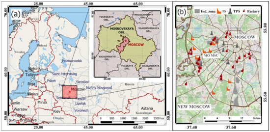
Figure 1.
(a) Location of Moscow in the European part of Russia. Insert at the right top is a map of Moscow City and Moscovskaya oblast. (b) Southwest sector of Moscow area including New Moscow. Location of sampling site at Meteorological Observatory of Moscow State University (MO MSU) (55°42′ N; 37°31′ E) is indicated. Industrial zones (Ind.zone), thermal power stations (TPS), thermal stations (TS) and factories (Factory) are shown.
Today, Moscow accounts for 10% of the Russian vehicle fleet, over 4.6 million cars were registered by the end of 2017 [49]. While automobilization is growing in Moscow, intensive implementation of higher ecological classes of engines, a declining share of trucks, and better quality of fuel promote the improvement of vehicle ecological parameters. Standards below the Euro-5 have been banned since January 2016. By 2014, up to 50% of motor fuels in Moscow corresponded to class 5. Over the past 7 years, large-scale road construction, development of public transport, and improvement of the structure of vehicle fleet led to a density of emissions does not exceed 500 tons/sq.km/year for 70% of the territory of a city [49]. Nevertheless, presently, the Moscow megacity often faces serious traffic congestion problems because of the vehicle number increasing. Economic losses due to traffic jams are significant, as a car stuck in a traffic congestion emits an average of 30% more pollutants [49].
Gaseous exhaust from automobile transport composes 93% of total megacity emissions [49]. Of industrial gaseous emissions, 50–65% relate to combined heat and power plants, producing and redistributing energy, gas, and water, 20–30% are emitted by refineries, and 15–20% by manufacturing industries. A remaining 2–3% of industrial gaseous emissions originate from the machinery and equipment industry, incinerators, food production, and construction. Heat and power plants, and the residential sector in a city are almost totally supplied with natural gas (gas composes 96.7% of fuel consumption), distinguishing Moscow from many European and Asian cities. In Moscovskaya Oblast the fraction of heat plant emissions is high, as much as 40% from the total stationary sources while the using of coal is significantly decreasing, different from Asian part of Russia [50].
The characteristic feature of Moscow is the high air pollution level in its northwest and northeast sectors where the main industrial and transportation sources are concentrated [30]. The Moscow center is cleaner despite heavy traffic because the absence of industrial enterprises. The lowest pollutant concentrations are observed in the southwestern sector which address the urban background.
In spring and summer, fires are usually observed in the European part of Russia and in the Moscow Oblast; they impact the aerosol properties as well [51]. The agriculture practice of the last year grass removing on fields is widespread in the spring season.
BB including waste burning is pronounced in residential areas around a city, especially during May holidays from 1 to 10 May, as recorded in 2017 and 2018–2019, in [33,36], respectively.
Measurement campaigns of this study are conducted at the Aerosol Complex located at the territory of the Meteorological Observatory of Moscow State University (MO MSU), southwest of Moscow city (Figure 1). MO MSU takes place at about 800 m south of a residential area and a highway. Industrial areas are situated at a distance of 3 km and greater from MO MSU. This enables the revealing the trends of aerosol composition as parameters of background urban pollution [47].
Real-time BC measurements were carried out at the MO MSU site with time resolution 1 min. Aerosol equivalent BC (eBC) concentrations were measured using custom made portable aethalometer. This instrument was purposely designed for mobile measurement campaigns and was successfully used at different platforms and in various regions [36,52,53].
The light attenuation caused by the particles depositing on a quartz fiber was analyzed at three wavelengths (450, 550, and 650 nm). eBC concentrations were determined by converting the time-resolved light attenuation to eBC mass at 650 nm and characterized by a specific mean mass attenuation coefficient, as described elsewhere [52].
Calibration parameter for quantification eBC mass was derived during parallel long-term measurements against an AE33 aethalometer (Magee Scientific) that operates at the same three wavelengths, for more details see elsewhere [36]. The light attenuation coefficient of the collected aerosol was calculated as
where is the filter exposed area and is the volume of air sampled and is the light attenuation defined as follows:
where and is the light intensity transmitted through unexposed and exposed parts of the filter, respectively. A wavelength of 660 nm was used further to represent eBC concentration. A good linear correlation between the aethalometer’s attenuation coefficient and the EBC concentrations calculated with the AE33 aethalometer (at 660 nm) was achieved ( This allowed estimation of EBC mass concentrations using the regression slope and intercept between at 650 nm and EBC of the AE33 aethalometer at 660 nm:
where is the correction factor that includes the specific mass absorption coefficient for the MSU aethalometer calibrated against the AE33 aethalometer assuming the Mass Absorption Cross section (MAC) adopted by AE33 equal to 9.89 m2 g−1. The uncertainty of EBC measurements from both aethalometers depends on the accuracy of the MAC value used for the conversion of the light absorption coefficient to mass concentration. The constant MAC value adopted here is an approximation, assuming a uniform state of mixing for BC in atmospheric aerosol. Absolute uncertainties of the reported MAC values remain as high as 30–70% due to the lack of appropriate reference methods.
Aethalometer filters were changed manually at the latest when ATN values approached 70 but at most times filters were changed at lower values. During rough and wet weather conditions, water droplets affected the measurements adding higher noise to the recorded ATN signal and big uncertainties. These short data periods were either excluded from the dataset or, where possible, treated manually by establishing an adjusted baseline for the reference ATN values. BC is commonly used as a term for black carbon, further we will use it instead eBC.
Particles with diameter less than 10 µm (PM10) were collected on 47 mm quartz fiber filters in 24 h intervals from 5 p.m. of a given day to 5 p.m. next day. Air was sampled at the flow of 16 l/min; the pumped volume was reported at standard atmosphere conditions. Measurements of meteorological parameters (temperature, relative humidity, pressure, precipitation, wind speed and wind direction) were performed each 3 h by MO MSU meteorological service.
Sampling campaigns were performed from the end of April 2019 until January 2020. The measurement time is divided on five periods with following designations: spring time from 30 April 2019 to 7 May 2019 (SPRING 1), spring time from 7 May 2019 to 31 May 2019 (SPRING 2), summer time from 1 June 2019 to 1 August 2019 (SUMMER), autumn time from 23 September 2019 to 30 November 2019 (AUTUMN), and winter time from 1 December 2019 to 19 January 2020 (WINTER). Central heating season ended on 7 May 2019 (when during 5 days temperature was higher 8 °C) and started again on 23 September 2019 (when during 5 days temperature was less 8 °C). Therefore, the separation of springtime into two periods relates to the ending of the heating system operation at the end of SPRING 1 period.
In order to compare the BC variabilities in spring 2019 using the pollution rose analyses with ones in spring of 2017 and 2018 [36], we combine SPRING1 and SPRING2 into one SPRING period. Because samples had not been collected for AAE measurements during spring of 2019 (due to technical reasons) we present here AAE data obtained for spring of 2018 (SPRING 2018) in order to complete the seasonal analyses for light absorption properties as well.
2.2. Meteorological Observations
Meteorological parameters (air temperature, water vapor pressure, precipitation, and wind speed) for separated seasonal periods of 2019 as well as for SPRING 2018 are presented in Table S1. Winter and autumn periods with averaged air temperature 0.4 °C and 5.4 °C, respectively, relate to cold seasons in Moscow. In order to describe meteorological parameters in comparison with previous years we calculated the deviations of their means from climatic ones in the period from 1981 to 2010, based on MO MSU observation data. Such deviations are called as “anomaly”.
The positive anomaly for air temperature during SPRING1 and SPRING2 periods was 1.5 °C and 3.6 °C, respectively. May of 2018 and 2019 were warmer by 3.0 °C and 2.9 °C than climatic mean, respectively. In May 2018, atmospheric pressure was increased due to the activity of the northeastern ridges of the Azores high while in May 2019 atmospheric pressure was low. The maximum air temperature in SPRING2 and SPRING 2018 periods was 29.2 °C on 29 May 2019 and 27.8 °C on 2 May 2018, respectively.
By contrast, during SUMMER the temperature was below than climatic mean by 0.3 °C. July was the coldest summer month. Its negative anomaly of 2.9 °C was associated with the displacement of Atlantic cyclones to the Arctic seas coast and the north of the European part of Russia. At that time the Moscow region was often affected by the northern and northwest air flows in the rear cold parts of cyclones. The maximum air temperature of 31.4 °C was observed in 8 June 2019.
Autumn had its warmest in the last 60 years due to stable anticyclonic weather in October and November, with anomaly air temperature 2.3 °C. Precipitation was below climatic mean in Autumn. In winter, anomaly air temperature approached 6.1 °C. The largest positive anomaly of monthly averaged air temperature was observed as high as 5.9 °C in December, due to the increased cyclonic activity over the North Atlantic area of the Icelandic low pressure. The snow covers in winter 2019–2020 was unstable, it was observed only during 22 days for the period. The average snow depth was 3 cm, the maximum snow depth was only 15 cm on 31 January 2020. Difference from the climatic means in the circulation conditions was in winter when the west wind was prevailed. Negative anomaly in the range 0.4–0.6 m/s was observed for the wind speed.
2.3. Methods and Analyses
Off-line examination of light attenuation on quartz filter samples was performed using a multiple-wavelength light transmission instrument (transmissometer), based on the method described in [54]. The intensity of light transmitted through quartz filters was measured at seven wavelengths from the near-ultraviolet to near-infrared spectral region. Five different spots were exposed to evaluate the homogeneity of the filter sample, and we repeated the measurements at least three times. This procedure provided uncertainties of ~10%. Then, the averaged attenuation (ATN) was used for the parametrization of the attenuation (ATN) dependence on the wavelength λ using a power law relationship:
where the Absorption Angstrom Exponent (AAE) is a measure of a strength of the spectral variation of aerosol light absorption. AAE is assigned to source-specific optical marker because aerosols produced by motor vehicles and biomass burning can be distinguished by different wavelength (λ) dependences in the light absorption [32,53,54].
ATN = kλ−AAE
Pollution rose techniques are well known as an informative way for identifications what is the direction that the highest pollutant concentrations associated are. Bivariate polar plot is a useful method for graphitic visualization of the joint wind speed direction dependence of aerosol concentrations [55]. This approach allows to trace the source location, preferably at scale ~1–10 km where the wind direction is remaining quasi-constant while back-trajectories provides a limited support thanks to the low spatial resolution of the model employed [54]. For bivariate polar plots construction, the wind data are partitioned into wind speed direction bins, and the mean concentration calculated for each bin. Wind direction intervals at 10 degrees and 30 wind speed intervals in the range 0 to 20 m s−1 capture the sufficient details of the concentration distribution. Smoothing techniques is chosen for the estimate of the square root-transformed concentrations as a function of the bivariate wind components. Plotting the concentration data in polar coordinates is useful for the purposes of source identification [56].
Traffic data were taken from TomTom maps and traffic data system https://www.tomtom.com/en_gb/traffic-index/moscow-traffic/, accessed on 20 November 2021. Traffic congestion is provided in % of time what a driver takes for a trip compared with free-flow travel times. TomTom provides hour-by-hour congestion averaged for each day of week.
Backward trajectories (BWT) were generated using NOAA Hybrid Single-Particle Lagrangian Integrated Trajectory (HYSPLIT) model of the Air Resources Laboratory (ARL) [57] with the coordinate resolution equal to 1° × 1° of latitude and longitude. The potential source areas were investigated using 2 day BWT for air masses arriving each one hour at 250 m height above ground level (A.G.L.). Such height corresponds to the level of the boundary layer in Moscow as taking place at 250–300 m, as evaluated in [30]. Concentration weighted trajectory (CWT) analysis is an effective tool that is combined with BWT data and pollutant concentrations to trace the source origin [18]. For each grid cell, the mean concentration of a pollutant species is calculated as follows:
where Cij is the average weighted concentration in the grid cell (i,j), i and j are grid indices, k is the index of trajectory, N is the total number of trajectories used, Ck is the pollutant concentration measured upon arrival of k trajectory, and τijk is the residence time of k trajectory in a grid cell (i,j). A high value of Cij means that air parcels passing over cell (i,j) would cause high concentrations at the receptor site.
Fire information was obtained from Resource Management System (FIRMS) operated by the NASA/GSFC Earth Science Data Information System (ESDIS) (https://firms.modaps.eosdis.nasa.gov/map, accessed on 1 November 2021). It is based on satellite observations which register the thermal spots (open fires) with temperature above 2000 K. For the best identification of fire location data, this work uses data arrays on the spatial location of fire centers from the Visible Infrared Imaging Radiometer Suite (VIIRS). Daily maps were related to the computed trajectories, providing a clear picture of the geographical location of fires nearby the trajectory pass not more than 500 km, with the several kilometer resolutions.
3. Results
3.1. Seasonal, Diurnal, and Weekly BC Concentrations
The time series of eBC concentrations during the seasons of 2019 and winter of 2020 are shown in Figure 2. The variations from 0.2 to 8.8 μg/m3 are observed for the whole duration of the study. The descriptive statistics for all seasons are presented in Table 1. The seasonal mean BC concentration for the whole period of study is 1.7 ± 1.4 μg/m3. Maximum mean BC equal to 2.2 ± 1.8 μg/m3 is observed in SPRING1, it is higher than in SPRING2, 1.8 ± 1.3 μg/m3, respectively, that can relate to the end of the heating period in Moscow.
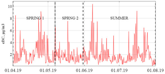
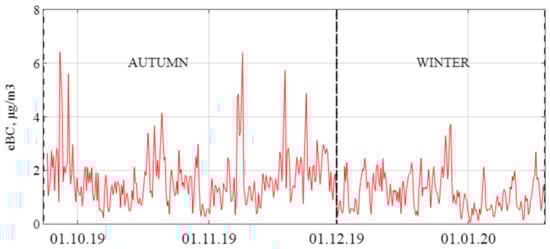
Figure 2.
Time series of 12 h mean eBC concentrations during SPRING 1, SPRING 2, SUMMER, AUTUMN and WINTER periods of 2019 and 2020 years. Dash lines separates the durations of periods.

Table 1.
Mean, maximum (max), and minimum (min) concentrations of black carbon (µg/m3) for separated seasonal periods of 2019 and 2020, and SPRING 2018; standard deviations (S.T.D.).
BC concentrations in SPRING 2018 [36] are summarized in Table 1 together with data for 2019. Mean of BC concentrations during approximately same periods of spring 2017 is found to be similar, 1.7 ± 1.4 μg/m3, to spring 2019. In spring 2018 the BC mean is smaller, 1.1 ± 0.9 μg/m3, than in spring 2019. For comparison, observations in the Moscow center in spring 2014 and 2016 showed the mean BC concentrations of 4.4 and 1.7 µg/m3 while at the suburban background station they were consistently less, 3.0 and 1.05 µg/m3, respectively [37]. In AUTUMN and WINTER periods, mean BC are lower, 1.7 ± 1.1 and 1.1 ± 0.7 μg/m3, than in SUMMER when mean BC is found 2.0 ± 1.8 μg/m3.
Seasonal BC in different cities of the globe brings out the importance of typical urban sources such as traffic, industry, heating, and residential emissions as well as of meteorology and the long-range transport over a particular location. Seasonal variations are found less pronounced in urban locations in Europe than in India and China [4]. In European less polluted cities such as Zurich, Basel, Gent, and Helsinki the seasonal variations in mean BC concentrations are observed from 1 to 2 µg/m3 [4,16] with maximums in fall and late winter due to the weakened mixing and enhanced emissions related to heating needs. In the Athens megacity, one of the most polluted cities in Europe, BC concentrations are equal to 2.4 ± 1.0 μg/m3 and 1.6 ± 0.6 μg/m3 during the cold and the warm period, respectively; the contribution from wood burning in residential sector is significantly higher during the cold period [5]. Observation of maxima in seasonal BC concentrations in spring in our study may indicate the particular impact of agriculture fires and long-range transport from surrounding regions (as will be shown later). Wintertime in 2019 and early 2020 was anomaly warm, therefore heating and energetic supplies operated at reduced potential.
The diurnal evolution of aerosols is influenced mainly by the space-time variation in atmospheric boundary layer (ABL) and source strengths of emissions. The ABL exhibits a definitive diurnal structure, its evolution over land is closely coupled with the heating of the surface by the Sun radiation. In urban environment, the atmospheric abundance of BC is affected by both the stability of the ABL and anthropogenic activities [4]. In large cities, the BC morning peak is well observed in diurnal mass concentrations; it is attributed to the combined influence of the ABL height and vehicle traffic enhancement in the morning [4,13,15]. The minimum BC concentrations is found during midday when there are fewer anthropogenic BC emissions, while the deeper boundary layer leads to a faster dispersion resulting in the pollution dilution. The surface inversion after sunset results in the accumulation of BC, causing even higher concentrations in the late evening.
In our study, the daily trend of BC concentrations differs in SPRING and SUMMER from AUTUMN and WINTER (Figure 3). In SPRING and SUMMER, a noticeable peak in concentrations exists in the morning between 6:00 and 9:00, relating to rush hours of traffic and maximum of the morning loading for heating and energy city supply. There is the daytime decrease to minimal values at approximately 15:00. A gradual growth in the evening to the night is observed after 20:00. We note that similar diurnal trend with a morning peak was observed in spring of 2017 [36]. There is a significant difference between maximum (around 3 µg/m3) in morning times and minimum (around 1 µg/m3) in daytime for diurnal trends in SPRING and SUMMER.
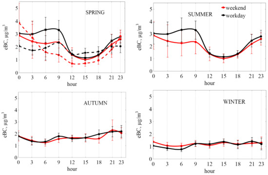
Figure 3.
Weekday and weekend diurnal variations of hourly black carbon concentrations during SPRING, SUMMER, AUTUMN, and WINTER periods. SPRING is separated on SPRING 1 (line) and SPRING 2 (stroke). Workdays and weekend are marked in black and red. Plotted points are average values for aggregated data from the subsequent three hours during each day of the study, standard deviation is show with error bars.
It is worth to consider the daily variations in CO concentrations, the most relevant to automobile emissions in Moscow. Due to the centralized heat supply of both residential and industrial sectors from large heat and power plants (HPP) using natural gas, the main source of CO in Moscow is automobile transport (approximately 85–90% of all emissions) [58]. CO daily variations measured during nine years at 49 stations in the Moscow megacity showed that on weekdays the CO concentrations reach daily maxima from 5:00 to 9:00 [58]. Such an increase is caused not only by heavy traffic but also their accumulations below the surface temperature inversion which is usually begins breaking up at 6:00–7:00 in summer. The similar diurnal trend we found for BC in SUMMER (Figure 3).
In AUTUMN and WINTER, the daily trend of BC concentrations is characterized by a smooth course and insignificant morning peak (Figure 3). The difference between maxima in morning times and minimum in daytime hardly approaches hundreds nanograms per m3. We note that in autumn and winter, the time of surface temperature inversion destroying is later, at 08:00–09:00. Such seasonal variation in temperature stratification may be responsible for absence of clear observed significant variation in diurnal trend in cold seasons.
In SPRING on weekends, the diurnal pattern is different considerably from that on weekdays (Figure 3). In SPRING 1 maximum values were measured in the morning. The biggest impact of weekend is observed in SPRING 2 (in the beginning of this period related to May holidays) by the prominent BC peak during morning rush hours in weekdays and almost its absent in weekend. We should note that Friday, Saturday, and Sunday are the most typical days for Moscow inhabitants to go out of the city for a weekend to their country houses and then back to a city. The raised nocturnal concentrations for weekend in SPRING 2 are caused by the numerous private cars travelling almost in evening and night hours. In SUMMER (a period of vacations), the differences between weekdays and weekend are not so prominent. We note that regular travels of inhabitants from Moscow city on weekends are typical for spring—summer seasons and less in autumn—winter. It is more specific and quite different from other European cites, for example, Helsinki, where high road traffic activity towards the suburbs of a city is observed during the whole year leading to the prominent weekend effect [16].
Weekly cycles of air quality are the characteristics of large cites related to the highest amount of pollutants emitted on working days. In SPRING, average BC of Tuesday, Wednesday and Thursday is much higher while in Friday its significant decrease is observed (Figure 4). Such a trend can be associated with the migration of the population from a city to the Moscovskaya Oblast for weekend. Moreover, SPRING 1, the period of central heating system operation, differs from SPRING2 by the more prominent morning peak that is related to higher emissions due to intensive energetic loading in the morning. The working activity in the middle of the week, in Thursday and Friday, is the most prominent in AUTUMN (Figure 4). In SUMMER and WINTER there is no strong difference between working days, always the minimum of BC relates to the weekend and Monday.
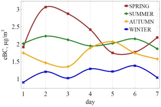
Figure 4.
Weekly trends of black carbon concentration during SPRING, SUMMER, AUTUMN, and WINTER periods.
During weekdays, a strong increase of traffic congestion, according Tom Tom system, well relates to a morning peak of BC while its decrease after 10:00 correlates with the BC drop (Figure 5). Correlation between BC and strong increase of traffic congestion is clearly observed after 15:00. High BC nocturnal level occurs mostly due to the shallow ABL resulting in the trapping of pollutants. Difference in population activity in a megacity is well demonstrated by the opposite correlation between traffic congestion and BC during weekend (Figure 5). Maximum transport activity happens at the middle of a day, contrary to a minimum of BC.

Figure 5.
Diurnal variations of hourly black carbon concentrations and Tom Tom traffic congestion during the whole period of study for weekdays (left) and weekend (right).
3.2. Relationships between BC and Meteorological Parameters
Wind roses for separated seasons of 2019 are shown in Figure S1. SPRING 1 is different from SPRING 2 by the eastern direction of prevailing winds. In SUMMER, the high frequency of northwestern (NW) winds are observed. AUTUMN and WINTER are similar by prevailing southwestern (SW) and western (W) winds.
The pollution roses show the variations of prevailed wind directions and BC concentrations from season to season (Figure 6). SPRING period is characterized by the most frequent NE and E wind directions with a repeatability frequency up to 18% and the highest BC concentrations from 6 to 12 μg/m3. During SUMMER, the maximum BC was observed from all wind directions with the highest frequency from the southwest. This finding confirms the observations of the SW prevailing wind direction in the air layer from 40 to 500 m at the MO MSU [59]. Pollution roses in AUTUMN and WINTER are similar with respect to the direction of the highest pollution concentrations. In WINTER, the NW direction with a repeatability frequency up to 35% occurs, the SW direction is observed more rarely while the maximum of BC approaches only 3 μg/m3.
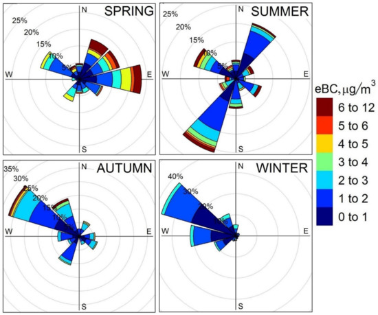
Figure 6.
Black carbon pollution roses during SPRING, SUMMER, AUTUMN, and WINTER periods.
Relationships among the source contribution, wind direction and speed are commonly derived from polar plots [60]. Figure 7 represents bivariate plots of BC concentrations in polar coordinates of wind speed and direction at the MO MSU, they indicate the origin of the main BC emission sources. Map in Figure 1 highlights the southwestern sector of Moscow city where the sampling site takes place. Industrial zones, thermal power stations (TPS), thermal stations (TS), and factories (of mechanical engineering, metallurgical, food production, reinforced concrete, chemical, and pharmaceutical) are shown, those ones which are located in the area around 10 km from the MO MSU. In WSW and N directions from the MO MSU the biggest industrial zones “Ochakovo” and “Fili” are located, respectively.
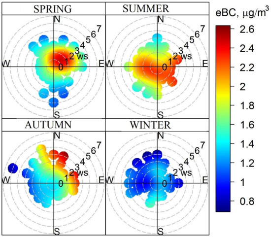
Figure 7.
Polar plots of BC concentrations for SPRING, SUMMER, AUTUMN, and WINTER periods (right). Wind speed (ws) is indicated in m/s.
In SPRING, the BC polar plot indicates the dominant influence of sources in the NE direction. Highest concentrations (above 2.2 µg/m3) occur at lowest wind speed during the days of windless weather, indicating the local emissions distributed around the MO MSU site. Such a picture is a typical feature of non-buoyant ground level sources as traffic. At wind speed ~2 m/s remote sources such as the industrial zone ”Fili”, a number of TPSs and TS, and factories could impact BC at the MO MSU when the site occurred downwind the emission stacks.
The SUMMER polar plot shows a similar picture such as the BC homogeneously distributed sources around the sampling site at all wind directions and wind speeds up to 2 m/s. It also identifies emissions from the NW and W direction of the industrial zone “Kunzevo’’ and “Ochakovo”, respectively. The biggest thermal power station in Moscow, TPS-25, is located in “Ochakovo”, its pollution dispersion area covers the territory of the MSU campus [61].
In AUTUMN, the situation is noticeably changed, its polar plot reveals the biggest impact from relatively remote sources in the NE at wind speeds higher than 2 m/s. A number of TPS takes place in this direction. The WINTER polar plot is characterized by the low BC concentrations (below 1.4 µg/m3) with homogeneous source distribution. Week (in comparison with other seasons) sources may be noted in the N and S directions.
Figure 8 shows BC pollution roses and polar plots separately for two spring periods, SPRING 1 and SPRING 2. The change of highest BC concentrations from the NE to NW, with a decrease of BC concentrations from the highest values (above 6 μg/m3) during the heating period to lower ones (below 4 μg/m3) after, is observed. On polar plots the highest BC concentrations during the heating period are observed at wind speed around 2 m/s, that indicates a source in the direction of the industrial zone “Fili” and a number of HPPs. The situation is noticeably changing after the end of the central heating system operation. BC concentrations decreased, and the origin of emission sources were changed to the NW, hardly identified at wind speeds above 2 m/s.
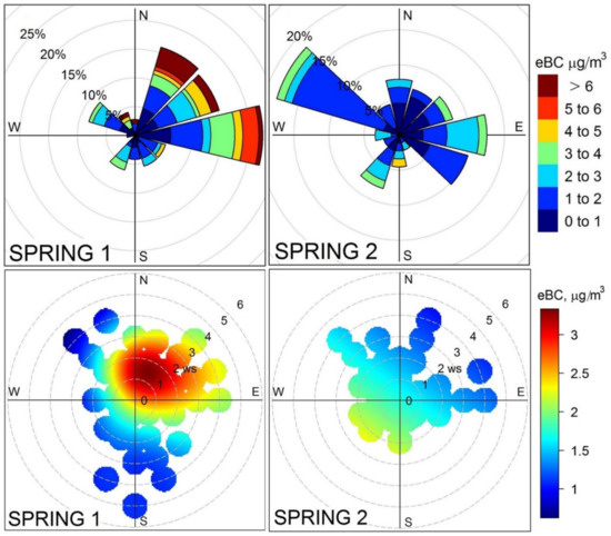
Figure 8.
Black carbon pollution roses (upper) and polar plots (bottom) for SPRING 1 and SPRING 2 periods.
3.3. Biomass Burning-Related Sources
Light absorption by particulates emitted from fossil fuel combustion sources exhibits a weak wavelength dependence with the Absorption Angstrom Exponent (AAE) close to 1.0 [2]. Wood smoke aerosols are distinguished by a strong wavelength dependency, showing AAE about 2.5. Large AAE near 4.0 indicates wood and debris burning in smoldering phase [62]. For ambient aerosols the study [43] recommended AAE values of 0.9 and 1.68 related to traffic and wood smoke, respectively, for specific wavelength pairs by comparing the BC source apportionment results using the Aethalometer model [25] with 14C measurements.
Observations in urban environment had related the AAE variation to biomass burning impact [54]. The increased AAE above 1.0 was suggested for identification of periods most affected by biomass burning [5], termed as “BB-affected”. Elevated light absorption with AAE up to 4.1 was observed in Moscow urban environment for days affected by peat burning plumes [32]. Parametrization of AAE relating to fossil fuel and biomass burning—affected values below 1.3 and high, above 1.3, values, respectively, has supported the contribution of traffic/industry and agriculture fires/residential biomass burning in Moscow urban background [34].
The spectral dependence of the aerosol light attenuation during a study period is well approximated by a power law equation (1), providing the estimate for AAE. Variation of AAE during SPRING 2018, and SUMMER 2019, AUTUMN 2019, and WINTER 2019–2020 exhibits the range from 0.6 to 1.9 (Figure 9). The seasonal maximum mean AAE is reached in WINTER 2019–2020 equal to 1.3 ± 0.2 (Table 2). Winter time is especially distinguished by the exceeding SPRING 2018, AUTUMN 2019, and SUMMER 2019 mean, max, and min values. New Year holidays (days of 01.01 and 02.01.2020), when fireworks use is very intensive, are clearly seen by AAE approaching 1.9. Frequency of observations with AAE > 1 is 98%, the highest one between other seasons.
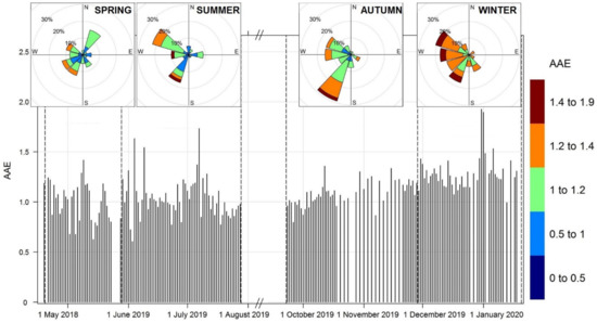
Figure 9.
Absorption Angstrom Exponent (AAE) during SPRING 2018, and SUMMER 2019, AUTUMN 2019 and WINTER 2019–2020. AAE roses for each period are presented.
Table 2.
Mean, maximum (max), and minimum (min) of Absorption Angstrom Exponent (AAE) during separated seasonal periods of 2019–2020 years and of SPRING 2018, standard deviations (S.T.D.), and frequency of observations for AAE > 1.
AUTUMN 2019 also demonstrates the high frequency of observations for AAE > 1, 78%. Together with WINTER 2019–2020, it reveals the biggest biomass burning impact in the cold seasons. At first sight, this finding looks surprising, considering that the local domestic heating using biomass burning is absent in Moscow megacity, in contrary from many other European cities, because the gas-fueled centralized heating supply continuously operates during the cold season. However, we should assume the strong influence of a huge residential area in the Moscovskaya Oblast located around the Moscow megacity.
In SPRING 2018 and SUMMER 2019, approximately the same mean AAE is obtained, 1.0 ± 0.2, with similar frequency of AAE > 1 observations, 58% and 50%, respectively. From 07 of May and during SUMMER periods the central heating system did not operate in Moscow. However, the warm period is traditionally related with the intensive weekend migration of population to the suburban area and also to vacation time when the elevated temperature stimulates the intensive residential activity around Moscow city such as garden cleaning, grass burning, and barbecue. Moreover, the spring season is traditional time for agriculture fires induced by grass burning on fields.
In a few days of study periods low AAE values were observed, even as low as 0.6 in SPRING 2018. Chemical evolution of aerosol mixing state, particle morphology, and size distribution after emissions and atmospheric aging can influence aerosol absorption, which can be noticed especially for the long-range transported air masses [63,64,65]. The AAE for the aged aerosols measured during a few periods as low as 0.6 could addressed mostly to the aerosol size distribution (large particles) and internally mixed BC particles [63]. As shown by modeling studies [66] pure BC particles coated by non-absorbing coating can have AAE in the range from <1 to 1.7, depending also on the morphology of the fractal aggregates [65].
Directions of the high AAE (above 1) indicated by AAE roses are SW, W, and NW in WINTER 2019 while only SW is dominant in AUTUMN 2018 (Figure 9). We should note that AAE roses do not show the similar direction as for BC concentrations for the same periods, see Figure 6 for comparison. This finding indicates that the biomass burning source does not impact much the BC concentrations in Moscow urban environment, having its own location distribution different from fossil fuel combustion. Moreover, the same directions but with lower AAE is observed in SPRING 2018 and SUMMER 2019.
3.4. Regional Sources of Black Carbon
Air masses arriving to a city may impact urban air quality, especially if the direction of their long-range transportation well correlates with fire-affected area. We use the CWT modeling to identify the origin of regional sources for observed high BC concentrations at the MO MSU site. Figure 10 shows CWT analyses for BC concentrations during four seasons of 2019–2020. In SPRING the source region of high concentrations (above 3 μg/m3) is extended far north and south, encompassing the large area of European part of Russia as a region of the BC origin. In SUMMER, the total area of high BC is reduced and localized into a dense area around Moscow megacity and stretched with a loop toward south. In AUTUMN and WINTER, sources for comparable high BC concentrations are no more observed, regions of lower (below 3 μg/m3) BC concentrations are rather homogeneous and large extended.
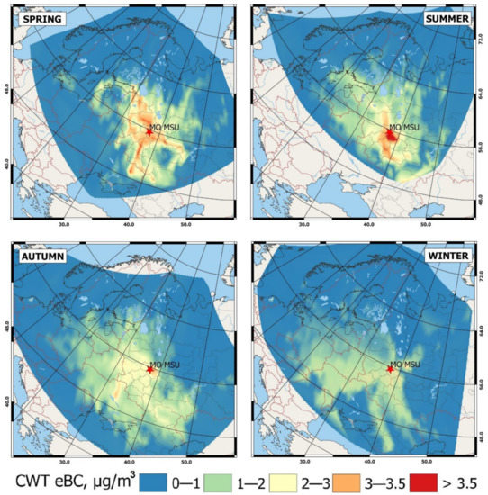
Figure 10.
Concentration weighted trajectory (CWT) analysis for black carbon during SPRING, SUMMER, AUTUM, and WINTER periods of 2019–2020 years. Color bars represent concentrations in μg/m3.
Fire activity is traditionally high in spring when temperature rises; agriculture practice with a purpose to remove the last year grass on the fields is widespread in this season. The majority of wildfire emissions occurs in the European part of Russia from March to late May [27]. In spring of 2018, the biggest number of open flaming fires occurred in the south-east direction from the Moscow area at the end of April [36]. Figure 11 shows backward trajectories of air mass transportation during days of increased AAE. Values above 1.3 were recorded at 8 May and 9 May in SPRING 2018 and at 1 June, 4 June, 6 June in SUMMER 2019, indicating the biggest biomass burning impact. The air mass transportation from areas with high fire activity is demonstrated: from northwest for 8 May and 1 June, from northeast for 9 May and 4 June, and from southwest for 6 July. Thus, AAE analyses in our study confirm that high atmospheric pollutions in Moscow could be mainly caused by the transport of biomass burning pollutions from the rural agricultural regions over a distance of hundred kilometers as well as from residential sector of Moscowskaya Oblact.
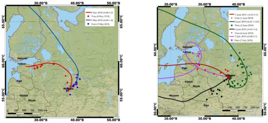
Figure 11.
Trajectories of air mass transportation during days of increased AAE above 1.3 in SPRING 2018 (left) and SUMMER 2019 (right), shown at 12:00 UTC. Fires near trajectory pathway at those days are indicated by the same color.
4. Conclusions
Moscow megacity is remaining to be low estimated densely populated source of potentially dangerous pollutants in the eastern part of Europe. A need to assess air quality in Moscow megacity led to the long real time BC measurements at the urban background site, on Aerosol Complex of MO MSU. Seasonal, weekly, and daily BC variations show the impact of urban sources, population activity, meteorology, and long-range transport over the site location. Level of BC in the range of seasonal variability similar to European cities indicates the comparable impacts of major urban sources such as traffic with intensive implementation of modern environmental requirements; heating power plants, producing and redistributing energy, gas, and water; and manufacturing industries. The specific source for Moscow megacity is the centralized heat supply for both residential and industrial sectors using natural gas.
Diurnal patterns in the spring and summer seasons shows the typical for large cities two peak structure during morning and evening hours when the atmospheric boundary layer (ABL) is shallow while traffic, heat, and energy supply are high. Seasonal variations in the ABL height and time of the surface temperature inversion smooth the diurnal trend in autumn and winter. BC has a weekly cycle with higher concentrations on weekdays relating to the largest combustion emissions on working days and a strong traffic congestion. Lower BC on Friday, Saturday, and Sunday is apparently related to the lower traffic rates and migration of the population from a city to the Moscovskaya Oblast for weekend.
Directions of the highest BC pollution concentrations are seasonally changed, as discovered by pollution roses. Polar plots indicate the origin of main BC emission sources nearby the MO MSU such as traffic, heating power plants, factories, and industrial zones in correlation with wind direction and wind speed. Parametrization of source-specific measure of spectral absorption, Angstrom Absorption Exponent (AAE), and its frequency of observations above 1 supports the seasonal source apportionment. The biggest impact of biomass burning occurs in the cold seasons (winter and autumn) that almost relates to the impact of a huge residential area around megacity while local domestic biomass burning is absent in Moscow. In the warm seasons of the elevated temperature, the weekend migration of population to the suburban area (particular activity of Moscow inhabitants) and vacation time stimulates the intensive residential BB activity around Moscow city. The transport of biomass burning aerosols from the rural agricultural fire-affected regions over a distance of hundred kilometers as well as from residential sector of peri-urban areas of Moscow can confirm high atmospheric BC pollutions in Moscow in spring and summer.
Supplementary Materials
The following supporting information can be downloaded at: https://www.mdpi.com/article/10.3390/atmos13040563/s1, Figure S1. Wind roses for SPRING 1, SPRING 2, SUMMER, AUTUMN, and WINTER periods. Wind rose for SPRING 2018 is shown in [36]; Table S1. Means of meteorological parameters: air temperature T(°C), water vapor pressure e (hPa), precipitation p (mm), and wind speed v (m/s) for separated seasonal periods of 2019 and SPRING 2018. Differences Δ with means in 1981–2010 years, according to Meteorological Obser-vatory MSU dataset.
Author Contributions
Conceptualization, original draft preparation and methodology, O.P.; data analyzing, software, and visualization, M.C., R.K. and E.Z.; supervision and editing, N.K. All authors have read and agreed to the published version of the manuscript.
Funding
This research: data collection and treatment was funded by Russian Science Foundation, grant number 19-77-300004. Methodology of aethalometer measurements and BC data analyses was implemented under a grant of the Ministry of Science and Higher Education of Russian Federation under the Agreement (075-15-2021-574).
Institutional Review Board Statement
Not applicable.
Informed Consent Statement
Not applicable.
Data Availability Statement
Not applicable.
Acknowledgments
This research was performed according to the Development program of the Interdisciplinary Scientific and Educational School of Lomonosov Moscow State University ⟪Future Planet and Global Environmental Change⟫, was carried out using the equipment of MSU Shared Research Equipment Center “Technologies for obtaining new nanostructured materials and their complex study” and purchased by MSU in the frame of the Equipment Renovation Program (National Project “Science”).
Conflicts of Interest
The authors declare no conflict of interest.
References
- Jacobson, M.Z. Short-term effects of controlling fossil-fuel soot, biofuel soot and gases, and methane on climate, Arctic ice, and air pollution health. J. Geophys. Res. Atmos. 2010, 115, D14209. [Google Scholar] [CrossRef]
- Kirchstetter, T.W.; Thatcher, T.L. Contribution of organic carbon to wood smoke particulate matter absorption of solar radiation. Atmos. Chem. Phys. 2012, 12, 6067–6072. [Google Scholar] [CrossRef]
- Mousavi, A.; Sowlat, M.H.; Hasheminassab, S.; Polidori, A.; Sioutas, C. Spatio-temporal trends and source apportionment of fossil fuel and biomass burning black carbon (BC) in the Los Angeles Basin. Sci. Total Environ. 2018, 640, 1231–1240. [Google Scholar] [CrossRef] [PubMed]
- Ramachandran, S.; Rajesh, T. Black carbon aerosol mass concentrations over Ahmedabad, an urban location in western India: Comparison with urban sites in Asia, Europe, Canada, and the United States. J. Geophys. Res. Atmos. 2007, 112, D06211. [Google Scholar] [CrossRef]
- Diapouli, E.; Kalogridis, A.-C.; Markantonaki, C.; Vratolis, S.; Fetfatzis, P.; Colombi, C.; Eleftheriadis, K. Annual Variability of Black Carbon Concentrations Originating from Biomass and Fossil Fuel Combustion for the Suburban Aerosol in Athens, Greece. Atmosphere 2017, 8, 234. [Google Scholar] [CrossRef]
- Janssen, N.A.H.; Hoek, G.; Simic-Lawson, M.; Fischer, P.; van Bree, L.; ten Brink, H.; Keuken, M.; Atkinson, R.W.; Anderson, H.R.; Brunekreef, B.; et al. Black Carbon as an Additional Indicator of the Adverse Health Effects of Airborne Particles Compared with PM(10) and PM(2.5). Environ. Health Perspect. 2011, 119, 1691–1699. [Google Scholar] [CrossRef] [PubMed]
- Popovicheva, O.B.; Kireeva, E.D.; Steiner, S.; Rothen-Rutishauser, B.; Persiantseva, N.M.; Timofeev, M.A.; Shonija, N.K.; Comte, P.; Czerwinski, J. Microstructure and chemical composition of diesel and biodiesel particle exhaust. Aerosol Air Qual. Res. 2014, 14, 1392–1401. [Google Scholar] [CrossRef]
- Popovicheva, O.B.; Kozlov, V.S.; Engling, G.; Diapouli, E.; Persiantseva, N.M.; Timofeev, M.; Fan, T.-S.; Saraga, D.; Eleftheriadis, K. Small-scale study of Siberian biomass burning: I. Smoke microstructure. Aerosol Air Qual. Res. 2015, 15, 117–128. [Google Scholar] [CrossRef]
- Maskey, S.; Chae, H.; Lee, K.; Dan, N.P.; Khoi, T.T.; Park, K. Morphological and elemental properties of urban aerosols among PM events and different traffic systems. J. Hazard. Mater. 2016, 317, 108–118. [Google Scholar] [CrossRef]
- Steiner, S.; Czerwinski, J.; Comte, P.; Popovicheva, O.; Kireeva, E.; Müller, L.; Heeb, N.; Mayer, A.; Fink, A.; Rothen-Rutishauser, B. Comparison of the toxicity of diesel exhaust produced by bio-and fossil diesel combustion in human lung cells in vitro. Atmos. Environ. 2013, 81, 380–388. [Google Scholar] [CrossRef]
- WHO. Health Effects of Black Carbon; WHO: Geneva, Switzerland, 2012. [Google Scholar]
- Chen, W.; Tian, H.; Qin, K. Black carbon aerosol in the industrial city of Xuzhou, China: Temporal characteristics and source appointment. Aerosol Air Qual. Res. 2019, 19, 794–811. [Google Scholar] [CrossRef]
- Chen, X.; Zhang, Z.; Engling, G.; Zhang, R.; Tao, J.; Lin, M.; Sang, X.; Chan, C.; Li, S.; Li, Y. Characterization of fine particulate black carbon in Guangzhou, a megacity of South China. Atmos. Pollut. Res. 2014, 5, 361–370. [Google Scholar] [CrossRef]
- Ramachandran, S.; Rajesh, T.; Cherian, R. Black carbon aerosols over source vs. background region: Atmospheric boundary layer influence, potential source regions, and model comparison. Atmos. Res. 2021, 256, 105573. [Google Scholar] [CrossRef]
- Kozlov, V.; Panchenko, M.; Yausheva, E. Diurnal variations of the submicron aerosol and black carbon in the near-ground layer. Atmos. Ocean. Opt. 2011, 24, 30–38. [Google Scholar] [CrossRef]
- Järvi, L.; Junninen, H.; Karppinen, A.; Hillamo, R.; Virkkula, A.; Mäkelä, T.; Pakkanen, T.; Kulmala, M. Temporal variations in black carbon concentrations with different time scales in Helsinki during 1996–2005. Atmos. Chem. Phys. 2008, 8, 1017–1027. [Google Scholar] [CrossRef]
- Tiwari, S.; Srivastava, A.K.; Bisht, D.S.; Parmita, P.; Srivastava, M.K.; Attri, S. Diurnal and seasonal variations of black carbon and PM2.5 over New Delhi, India: Influence of meteorology. Atmos. Res. 2013, 125, 50–62. [Google Scholar] [CrossRef]
- Bian, Q.; Alharbi, B.; Shareef, M.M.; Husain, T.; Pasha, M.J.; Atwood, S.A.; Kreidenweis, S.M. Sources of PM 2.5 carbonaceous aerosol in Riyadh, Saudi Arabia. Atmos. Chem. Phys. 2018, 18, 3969–3985. [Google Scholar] [CrossRef]
- Diapouli, E.; Popovicheva, O.; Kistler, M.; Vratolis, S.; Persiantseva, N.; Timofeev, M.; Kasper-Giebl, A.; Eleftheriadis, K. Physicochemical characterization of aged biomass burning aerosol after long-range transport to Greece from large scale wildfires in Russia and surrounding regions, Summer 2010. Atmos. Environ. 2014, 96, 393–404. [Google Scholar] [CrossRef]
- Sparks, T.L.; Wagner, J. Composition of particulate matter during a wildfire smoke episode in an urban area. Aerosol Sci. Technol. 2021, 55, 734–747. [Google Scholar] [CrossRef]
- Engling, G.; He, J.; Betha, R.; Balasubramanian, R. Assessing the regional impact of indonesian biomass burning emissions based on organic molecular tracers and chemical mass balance modeling. Atmos. Chem. Phys. 2014, 14, 8043–8054. [Google Scholar] [CrossRef]
- Ulevicius, V.; Byčenkienė, S.; Bozzetti, C.; Vlachou, A.; Plauškaitė, K.; Mordas, G.; Dudoitis, V.; Abbaszade, G.; Remeikis, V.; Garbaras, A.; et al. Fossil and non-fossil source contributions to atmospheric carbonaceous aerosols during extreme spring grassland fires in Eastern Europe. Atmos. Chem. Phys. 2016, 16, 5513–5529. [Google Scholar] [CrossRef]
- Liu, Y.; Yan, C.; Zheng, M. Source apportionment of black carbon during winter in Beijing. Sci. Total Environ. 2018, 618, 531–541. [Google Scholar] [CrossRef] [PubMed]
- Zhang, K.M.; Allen, G.; Yang, B.; Chen, G.; Gu, J.; Schwab, J.; Felton, D.; Rattigan, O. Joint measurements of PM 2. 5 and light-absorptive PM in woodsmoke-dominated ambient and plume environments. Atmos. Chem. Phys. 2017, 17, 11441–11452. [Google Scholar] [CrossRef]
- Sandradewi, J.; Prévôt, A.S.; Szidat, S.; Perron, N.; Alfarra, M.R.; Lanz, V.A.; Weingartner, E.; Baltensperger, U. Using aerosol light absorption measurements for the quantitative determination of wood burning and traffic emission contributions to particulate matter. Environ. Sci. Technol. 2008, 42, 3316–3323. [Google Scholar] [CrossRef] [PubMed]
- Massabò, D.; Caponi, L.; Bernardoni, V.; Bove, M.; Brotto, P.; Calzolai, G.; Cassola, F.; Chiari, M.; Fedi, M.; Fermo, P. Multi-wavelength optical determination of black and brown carbon in atmospheric aerosols. Atmos. Environ. 2015, 108, 1–12. [Google Scholar] [CrossRef]
- Huang, K.; Fu, J.S.; Prikhodko, V.Y.; Storey, J.M.; Romanov, A.; Hodson, E.L.; Cresko, J.; Morozova, I.; Ignatieva, Y.; Cabaniss, J. Russian anthropogenic black carbon: Emission reconstruction and Arctic black carbon simulation. J. Geophys. Res. Atmos. 2015, 120, 11306–11333. [Google Scholar] [CrossRef]
- Hao, W.M.; Petkov, A.; Nordgren, B.L.; Corley, R.E.; Silverstein, R.P.; Urbanski, S.P.; Evangeliou, N.; Balkanski, Y.; Kinder, B.L. Daily black carbon emissions from fires in northern Eurasia for 2002–2015. Geosci. Model Dev. 2016, 9, 4461–4474. [Google Scholar] [CrossRef]
- Cheng, Z.; Luo, L.; Wang, S.; Wang, Y.; Sharma, S.; Shimadera, H.; Wang, X.; Bressi, M.; de Miranda, R.M.; Jiang, J.; et al. Status and characteristics of ambient PM2.5 pollution in global megacities. Environ. Int. 2016, 89, 212–221. [Google Scholar] [CrossRef]
- Elansky, N.F.; Ponomarev, N.A.; Verevkin, Y.M. Air quality and pollutant emissions in the Moscow megacity in 2005–2014. Atmos. Environ. 2018, 175, 54–64. [Google Scholar] [CrossRef]
- Popovicheva, O.B.; Kistler, M.; Kireeva, E.; Persiantseva, N.; Timofeev, M.; Kopeikin, V.; Kasper-Giebl, A. Physicochemical characterization of smoke aerosol during large-scale wildfires: Extreme event of August 2010 in Moscow. Atmos. Environ. 2014, 96, 405–414. [Google Scholar] [CrossRef]
- Popovicheva, O.B.; Engling, G.; Ku, I.-T.; Timofeev, M.A.; Shonija, N.K. Aerosol Emissions from Long-lasting Smoldering of Boreal Peatlands: Chemical Composition, Markers, and Microstructure. Aerosol Air Qual. Res. 2019, 19, 484–503. [Google Scholar] [CrossRef]
- Popovicheva, O.; Padoan, S.; Schnelle-Kreis, J.; Nguyen, D.-L.; Adam, T.; Kistler, M.; Steinkogler, T.; Kasper-Giebl, A.; Zimmermann, R.; Chubarova, N. Spring Aerosol in the Urban Atmosphere of a Megacity: Analytical and Statistical Assessment for Source Impacts. Aerosol Air Qual. Res. 2020, 20, 702–719. [Google Scholar] [CrossRef]
- Popovicheva, O.; Ivanov, A.; Vojtisek, M. Functional Factors of Biomass Burning Contribution to Spring Aerosol Composition in a Megacity: Combined FTIR-PCA Analyses. Atmosphere 2020, 11, 319. [Google Scholar] [CrossRef]
- Golitsyn, G.S.; Grechko, E.I.; Wang, G.; Wang, P.; Dzhola, A.V.; Emilenko, A.S.; Kopeikin, V.M.; Rakitin, V.S.; Safronov, A.N.; Fokeeva, E.V. Studying the pollution of Moscow and Beijing atmospheres with carbon monoxide and aerosol. Izv. Atmos. Ocean. Phys. 2015, 51, 1–11. [Google Scholar] [CrossRef]
- Popovicheva, O.B.; Volpert, E.; Sitnikov, N.M.; Chichaeva, M.A.; Padoan, S. Black carbon in spring aerosols of Moscow urban background. Geogr. Environ. Sustain. 2020, 13, 233–243. [Google Scholar] [CrossRef]
- Kopeikin, V.; Emilenko, A.; Isakov, A.; Loskutova, O.; Ponomareva, T.Y. Variability of Soot and Fine Aerosol in the Moscow Region in 2014–2016. Atmos. Ocean. Opt. 2018, 31, 243–249. [Google Scholar] [CrossRef]
- Kopeikin, V.; Ponomareva, T.Y. Dependence of Variations in Black Carbon Content in the Atmosphere of Moscow on Air Mass Transport Direction. Atmos. Ocean. Opt. 2021, 34, 74–80. [Google Scholar] [CrossRef]
- Zhang, W.; Lu, Z.; Xu, Y.; Wang, C.; Gu, Y.; Xu, H.; Streets, D.G. Black carbon emissions from biomass and coal in rural China. Atmos. Environ. 2018, 176, 158–170. [Google Scholar] [CrossRef]
- Zhang, W.; Wang, J.; Xu, Y.; Wang, C.; Streets, D.G. Analyzing the spatio-temporal variation of the CO2 emissions from district heating systems with “Coal-to-Gas” transition: Evidence from GTWR model and satellite data in China. Sci. Total Environ. 2022, 803, 150083. [Google Scholar] [CrossRef]
- Briggs, N.L.; Long, C.M. Critical review of black carbon and elemental carbon source apportionment in Europe and the United States. Atmos. Environ. 2016, 144, 409–427. [Google Scholar] [CrossRef]
- Kalogridis, A.-C.; Vratolis, S.; Liakakou, E.; Gerasopoulos, E.; Mihalopoulos, N.; Eleftheriadis, K. Assessment of wood burning versus fossil fuel contribution to wintertime black carbon and carbon monoxide concentrations in Athens, Greece. Atmos. Chem. Phys. 2018, 18, 10219–10236. [Google Scholar] [CrossRef]
- Zotter, P.; Herich, H.; Gysel, M.; El-Haddad, I.; Zhang, Y.; Močnik, G.; Hüglin, C.; Baltensperger, U.; Szidat, S.; Prévôt, A.S. Evaluation of the absorption Ångström exponents for traffic and wood burning in the Aethalometer-based source apportionment using radiocarbon measurements of ambient aerosol. Atmos. Chem. Phys. 2017, 17, 4229–4249. [Google Scholar] [CrossRef]
- Pietrogrande, M.C.; Abbaszade, G.; Schnelle-Kreis, J.; Bacco, D.; Mercuriali, M.; Zimmermann, R. Seasonal variation and source estimation of organic compounds in urban aerosol of Augsburg, Germany. Environ. Pollut. 2011, 159, 1861–1868. [Google Scholar] [CrossRef] [PubMed]
- Cheng, Y.; Engling, G.; He, K.-B.; Duan, F.-K.; Ma, Y.-L.; Du, Z.-Y.; Liu, J.-M.; Zheng, M.; Weber, R.J. Biomass burning contribution to Beijing aerosol. Atmos. Chem. Phys. 2013, 13, 7765–7781. [Google Scholar] [CrossRef]
- Elansky, N.; Lavrova, O.; Rakin, A.; Skorokhod, A. Anthropogenic disturbances of the atmosphere in Moscow region. In Doklady Earth Sciences; Springer Nature: Berlin/Heidelberg, Germany, 2014; Volume 454, pp. 158–166. [Google Scholar]
- Chubarova, N.E.; Androsova, E.E.; Kirsanov, A.A.; Vogel, B.; Vogel, H.; Popovicheva, O.B.; Rivin, G.S. Aerosol and its radiative effects during the Aeroradcity 2018 Moscow experiment. Geogr. Environ. Sustain. 2019, 12, 114–131. [Google Scholar] [CrossRef][Green Version]
- Kuznetsova, I.; Konovalov, I.; Glazkova, A.; Nakhaev, M.; Zaripov, R.; Lezina, E.; Zvyagintsev, A.; Beekmann, M. Observed and calculated variability of the particulate matter concentration in Moscow and in Zelenograd. Russ. Meteorol. Hydrol. 2011, 36, 175–184. [Google Scholar] [CrossRef]
- Bityukova, V.R.; Mozgunov, N.A. Spatial features transformation of emission from motor vehicles in Moscow. Geogr. Environ. Sustain. 2019, 12, 57–73. [Google Scholar] [CrossRef]
- Bityukova, V.R.; Dehnich, V.S.; Petuhova, N.V. Impact of regional power plants on air pollution in Russian cities. Vestn. Mosk. Universiteta. Ser. 5 Geogr. 2021, 4, 38–50. [Google Scholar]
- Chubarova, N.; Smirnov, A.; Holben, B. Aerosol properties in Moscow according to 10 years of AERONET measurements at the Meteorological Observatory of Moscow State University. Geogr. Environ. Sustain. 2011, 4, 19–32. [Google Scholar] [CrossRef]
- Popovicheva, O.B.; Evangeliou, N.; Eleftheriadis, K.; Kalogridis, A.C.; Sitnikov, N.; Eckhardt, S.; Stohl, A. Black Carbon Sources Constrained by Observations in the Russian High Arctic. Environ. Sci. Technol. 2017, 51, 3871–3879. [Google Scholar] [CrossRef]
- Kirchstetter, T.W.; Novakov, T.; Hobbs, P.V. Evidence that the spectral dependence of light absorption by aerosols is affected by organic carbon. J. Geophys. Res. Atmos. 2004, 109, D21208. [Google Scholar] [CrossRef]
- Popovicheva, O.B.; Shonija, N.K.; Persiantseva, N.; Timofeev, M.; Diapouli, E.; Eleftheriadis, K.; Borgese, L.; Nguyen, X.A. Aerosol Pollutants during Agricultural Biomass Burning: A Case Study in Ba Vi Region in Hanoi, Vietnam. Aerosol Air Qual. Res. 2017, 17, 2762–2779. [Google Scholar] [CrossRef]
- Uria-Tellaetxe, I.; Carslaw, D.C. Conditional bivariate probability function for source identification. Environ. Model. Softw. 2014, 59, 1–9. [Google Scholar] [CrossRef]
- Carslaw, D.C.; Beevers, S.D. Characterising and understanding emission sources using bivariate polar plots and k-means clustering. Environ. Model. Softw. 2013, 40, 325–329. [Google Scholar] [CrossRef]
- Stein, A.; Draxler, R.; Rolph, G.; Stunder, B.; Cohen, M.; Ngan, F. NOAA’s HYSPLIT atmospheric transport and dispersion modeling system. Bull. Am. Meteorol. Soc. 2015, 96, 2059–2077. [Google Scholar] [CrossRef]
- Elansky, N.; Shilkin, A.; Ponomarev, N.; Semutnikova, E.; Zakharova, P. Weekly patterns and weekend effects of air pollution in the Moscow megacity. Atmos. Environ. 2020, 224, 117303. [Google Scholar] [CrossRef]
- Lokoshchenko, M. Wind direction in Moscow. Russ. Meteorol. Hydrol. 2015, 40, 639–646. [Google Scholar] [CrossRef]
- Saraga, D.; Maggos, T.; Degrendele, C.; Klánová, J.; Horvat, M.; Kocman, D.; Kanduč, T.; Dos Santos, S.G.; Franco, R.; Gómez, P.M. Multi-city comparative PM2.5 source apportionment for fifteen sites in Europe: The ICARUS project. Sci. Total Environ. 2021, 751, 141855. [Google Scholar] [CrossRef]
- Bityukova, V. Spatial structure of pollution areas from combined heat and power plant (CHP) in Moscow. Ecol. Ind. Russ. 2021, 25, 54–60. [Google Scholar] [CrossRef]
- Popovicheva, O.; Kozlov, V. Impact of combustion phase on scattering and spectral absorption of Siberian biomass burning: Studies in Large Aerosol Chamber. In Proceedings of the SPIE 11560, 26th International Symposium on Atmospheric and Ocean Optics, Atmospheric Physics, Moscow, Russia, 6–10 July 2020; p. 115604N. [Google Scholar]
- Cappa, C.D.; Kolesar, K.R.; Zhang, X.; Atkinson, D.B.; Pekour, M.S.; Zaveri, R.A.; Zelenyuk, A.; Zhang, Q. Understanding the optical properties of ambient sub- and supermicron particulate matter: Results from the CARES 2010 field study in northern California. Atmos. Chem. Phys. 2016, 16, 6511–6535. [Google Scholar] [CrossRef]
- Saleh, R.; Hennigan, C.; McMeeking, G.; Chuang, W.; Robinson, E.; Coe, H.; Donahue, N.; Robinson, A. Absorptivity of brown carbon in fresh and photo-chemically aged biomass-burning emissions. Atmos. Chem. Phys. 2013, 13, 7683–7693. [Google Scholar] [CrossRef]
- Romshoo, B.; Müller, T.; Pfeifer, S.; Saturno, J.; Nowak, A.; Ciupek, K.; Quincey, P.; Wiedensohler, A. Optical properties of coated black carbon aggregates: Numerical simulations, radiative forcing estimates, and size-resolved parameterization scheme. Atmos. Chem. Phys. 2021, 21, 12989–13010. [Google Scholar] [CrossRef]
- Virkkula, A. Modeled source apportionment of black carbon particles coated with a light-scattering shell. Atmos. Meas. Tech. 2021, 14, 3707–3719. [Google Scholar] [CrossRef]
Publisher’s Note: MDPI stays neutral with regard to jurisdictional claims in published maps and institutional affiliations. |
© 2022 by the authors. Licensee MDPI, Basel, Switzerland. This article is an open access article distributed under the terms and conditions of the Creative Commons Attribution (CC BY) license (https://creativecommons.org/licenses/by/4.0/).