Abstract
Urban air chemistry is characterized by measurements of gas and aerosol composition. These measurements are interpreted from a long history for laboratory and theoretical studies integrating chemical processes with reactant (or emissions) sources, meteorology and air surface interaction. The knowledge of these latter elements and their changes have enabled chemists to quantitatively account for the averages and variability of chemical indicators. To date, the changes are consistent with dominating energy-related emissions for more than 50 years of gas phase photochemistry and associated reactions forming and evolving aerosols. Future changes are expected to continue focusing on energy resources and transportation in most cities. Extreme meteorological conditions combined with urban surface exchange are also likely to become increasingly important factors affecting atmospheric composition, accounting for the past leads to projecting future conditions. The potential evolution of urban air chemistry can be followed with three approaches using observations and chemical transport modeling. The first approach projects future changes using long term indicator data compared with the emission estimates. The second approach applies advanced measurement analysis of the ambient data. Examples include statistical modeling or evaluation derived from chemical mechanisms. The third method, verified with observations, employs a comparison of the deterministic models of chemistry, emission futures, urban meteorology and urban infrastructure changes for future insight.
1. Introduction
Atmospheric chemistry began in the mid-18th century with Rutherford’s discovery of nitrogen dioxide (NO2) and Priestley’s discovery of oxygen in air. Air chemistry expanded after the 19th century with Smith’s [1] acid rain research in England, ozone formation [2] and airborne particles or nuclei [3,4]. Contemporary tropospheric chemistry began to expand with meteorology after the Second World War [5]. A special case focusing on urban conditions emerged driven by increasing concerns for adverse health effects associated with air pollution exposure.
As Roy Harrison [6] noted: “Studies of the chemistry of the urban atmosphere provide special challenges which arise from the high density of emissions, strong concentration gradients and relatively high pollutant concentrations. In contrast to the regional and global atmosphere, local dispersion processes (meteorology) play a much larger role in determining atmospheric concentrations and also have substantial effect on chemical transformations. On the other hand, residence times in the urban atmosphere are relatively short, hence limiting the range of chemical reaction processes which are significant. Some key species such as the hydroxyl radical have different predominant source processes in the urban and regional atmosphere. A case is made that the differences are so large that urban atmospheric chemistry needs to be given special treatment and cannot simply be considered as subtly different from regional and global atmosphere studies”.
Chemical species found in urban air have been identified with virtually every human activity. One group of chemicals are identified historically with air pollution from energy production and use, including the emission and combustion of fossil fuels. Urban air chemistry initially focused on well-known sulfurous by-products of fuel combustion. Widespread severe pollution events associated with sulfur oxides were recorded in fogs of London [5], and in Donora, Pennsylvania in 1948 [7]. In the 1950s, sunlight-induced smog was identified with oxidants in southern California [8]. As a result of regulatory pressure; e.g., the 1956 British Clean Air Act [5] and the U.S. Clean Air Acts [9,10], the study of urban air chemistry increased dramatically after the 1960s. As a result of such studies, it was widely recognized that indicators of urban chemistry were dependent not only on chemical mechanisms and reactants (emissions), but also on certain unique meteorological conditions.
In most early studies of urban air chemistry, characteristic meteorological conditions were specified, while the influence of gaseous or particle pollution emissions were varied to seek control strategies for air quality improvement. Since the 1950s, the chemical mechanisms of reactive gas oxidation have been characterized in great detail [11,12]. Early on, urban air chemistry recognized the importance of an airborne particle (aerosol) component. Aerosols drive both from primary sources and from the oxidation of gases that link with gas phase chemistry [13]. Mechanisms for aerosol formation were predicated for inorganic components by the 1980s. However, knowledge of the complexities of organic aerosols has expanded dramatically since the 1990s [14,15].
During the course of studies after the 1970s, estimates of the change in ambient composition using models combining emissions, meteorology and chemistry along with measurements were made to characterize the spatial and temporal distributions of gas and aerosol properties. These studies created a large data base for forecasting changes in the composition of the urban atmosphere mainly with changes in a relatively constrained “business-as-usual” range of pollutant emissions. Business-as-usual focused mainly on a carbon basis for energy production and for transportation. In contemporary studies, the notion of “change” has expanded to include not only apparent climate induced meteorological change, but also the potential influence of dramatic changes in energy resources resulting from decarbonization, with forms of transportation that do not rely on fossil fuels.
In addition to considering the results of major shifts in energy-related emissions for gases and aerosols, there continue to be contemporary issues for new knowledge. For gases, these include: (a) ozone chemistry in the VOC sensitive range, and (b) nocturnal and seasonal differences in photochemistry. For aerosols, example issues include: (a) characterization of organic species and chemistry for primary and secondary sources, (b) interaction with aqueous particles, and (c) characterizing surface properties of particles for the reactivity of heterogeneous processes.
In this paper, a framework is presented to account for the change in energy-related urban air chemistry that embodies meteorology, reactants and mechanisms. A response to such changes can be described using three modes of study. These include investigation, based on trends in gas and particle composition, the interpretation of mechanisms through atmospheric measurement campaigns, and the application of modeling with expanded hypothetical meteorological and emissions changes. The basic gas phase chemical mechanisms of interest are assumed to be principally unchanged. However, it is anticipated that aerosol source and formation mechanisms will continue to evolve with advancing knowledge.
2. A Menu for Urban Air Chemical Change
2.1. Urban Air Chemistry
Urban chemistry changes could involve a wide range of constituents, including community chemical reactants—pollutants, toxins, biological species and non-local contaminants. For the purposes of this study, we constrain the discussion to community pollutants mainly in the oxidant cycle and in aerosol composition by mass concentration. Example cities with different “significant air chemistry” (pollution) conditions as characterized by certain reactant-product indicators are listed in Table 1. The data in this table suggests a range of chemical indicator concentrations expected across the world. For the purposes of this study, we concentrate on U.S. domestic examples.
The chemicals of interest in tracking the results of change are listed in Table 1 (gas phase) and Table 2 (aerosol or particles). Most of species listed in Table 1 are associated primarily with the chemical mechanisms characterizing photochemical oxidant formation. For aerosols, the chemistry is complicated by the fact that particulate composition in cities depends not only on atmospheric reactions, but also the injection of a variety of particles from primary sources that enable the potential for heterogeneous reactions to take place. We noted that urban conditions cannot be considered in isolation. They are increasingly influenced by a so-called regional or continental background [16,17,18]. Among the key elements of regional background are not only downwind transport from cities, but also [19] the major dust storms in China [20] and widespread wildfires across Asia, Africa and the United States [21].
As a framework, it is useful to keep in mind the photochemically related chemistry prevalent in the troposphere, which includes the interaction of gas phase and aerosol products. A common textbook example showing these interactions in the photochemical cycle is shown in Figure 1. As noted above, this chemistry and its response to changes in nitrogen oxide (NOx [= NO + NO2]) and volatile organic compound (VOC) precursor emissions between the 1960s and today are likely indicators for future changes. The measurements of these constituents could be supplemented with additional research-oriented measurements, including hydoxyl radical (OH) and peroxides. Equally important for tracking change is the composition of VOC (Table 3), and the measures of their reactivity (such as OH reactivity) with an increasing reduction in these species with emission reductions [22].
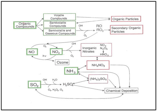
Figure 1.
Schematic diagram for gas phase and particle interactions in common chemical cycles relevant to the urban atmosphere, for example, the photochemically related cycle. Note the gas phase dominance to produce O3 and the aerosol linkages to SO2, NOx oxidation and OC production in the upper right. (From [22]; courtesy of Cambridge University Press).
Aerosol chemistry indicators include a variety of particles, including electric power generation, vehicle exhaust, industrial emissions, space heating, cooking smoke, wildfires and vehicle tire wear (Table 2). Well-known secondary sources of particles include the oxidized inorganic gas products, such as sulfate (SO4) and particle nitrate (NO3) identified primarily as ammonium salts, and condensed organic carbon (OC) species.
Regional or continental background chemistry is increasingly important to urban chemistry as initial conditions for local chemistry, and for setting baselines below which urban air composition is constrained. Background chemistry can include the species listed in Table 1, Table 2 and Table 3, but at lower concentrations than is found locally in cities.

Table 1.
Examples of gas phase components as key indicators of the chemical processes associated with urban pollution and background chemistry. Species in bold are routinely monitored.
Table 1.
Examples of gas phase components as key indicators of the chemical processes associated with urban pollution and background chemistry. Species in bold are routinely monitored.
| Gas | Chemistry | Sources | Hypothetical Change e |
|---|---|---|---|
| Carbon monoxide (CO) | Long lived slow reacting combustion tracer | Carbon fuel combustion | ↓ |
| Sulfur dioxide (SO2) | Sulfate reactant; oxidized in oxidant cycle | Fossil fuel contaminant | ↓ |
| Nitric oxide (NO) | Oxidant cycle | Fossil fuel combustion; power plants, vehicles; biomass burning | ↓ |
| Nitrogen dioxide (NO2) | Oxidant cycle; product of O3-NO reaction | Fossil fuel combustion; biomass burning | ↓ |
| Non-methane HC (NMHC) a | Part of VOC c; reactant for oxidant cycle | Incomplete combustion; industrial–commercial; vegetation | ↓ |
| Ozone (O3) | Oxidant photochemistry | Product of oxidant cycle | →? d |
| Nitric acid (HONO2) | Oxidant cycle | ↓ | |
| Organo-nitrates (e.g., PAN) | Oxidant cycle | Reactions of VOC and NOy | ↓? |
| Ammonia (NH3) | Cation for acid species | Agriculture; natural | ? |
| Formaldehyde and other aldehydes | Product of oxidant cycle | VOC oxidation; biomass burn | ↓? |
| Acetone | Product of oxidant cycle | VOC oxidation | ↓? |
| Acetylene | Combustion tracer | Auto exhaust | ↓ |
| H2O2 | Oxidant photochemistry | Product of oxidant cycle | →? |
| OH | Key product in oxidant cycle | Intermediate in O3 cycle | →? |
| RO2 b | Key product in oxidant cycle | Intermediate in O3 cycle | →? |
a Generic for large number of hydrocarbon species; many associated with motor vehicle exhaust. b Peroxides; R is the alkyl group. c Volatile organic compounds; includes NMHC. d Depends on the frequency of occurrence of extreme values vs. mean concentration. e Hypothetical change with contemporary reactant reductions, chemical mechanisms are the same as today, and continued dominance of natural gas for energy production, and gasoline or distillate fuel use as shown in [23] projections.
Table 2.
Particle measures potentially associated with urban chemistry, including representatives of primary and secondary sources. Species in bold are routinely monitored. Particle nitrate requires special measurement because of its volatility as NH4NO3.
Table 2.
Particle measures potentially associated with urban chemistry, including representatives of primary and secondary sources. Species in bold are routinely monitored. Particle nitrate requires special measurement because of its volatility as NH4NO3.
| PM2.5 Species | Chemistry | Sources | Hypothetical Change |
|---|---|---|---|
| PMx mass | |||
| Black carbon (BC) | Assumed inert but surface may be active | Incomplete combustion-fossil and biomass C | ↓? Affected by wildfires, reduced from improved combustion tech. |
| Organic carbon (OC) (Hydrocarbon rich; oxygen rich) | Primary species potentially oxidized; coupled to oxidant cycle VOC reactions | Incomplete combustion; vegetation emissions | ↓? Improved combustion tech., but natural VOC potentially important |
| Sulfate (SO4) | Product of sulfur gas oxidation by gas phase or heterogeneous reactions | Derived from SO2; gas from combustion of fossil fuel | ↓ |
| Nitrate (NO3) | Linked with oxidant cycle to form HNO3, NO3 and N2O5. | Traced to NOx from fuel combustion | ↓ |
| Ammonium (NH4) | Acid neutralization | Agriculture | → |
| Soil dust related species | Assumed inert, but potential for surface reactions | Road dust and blowing soil; cement production | ↑? |
| NaCl | Assumed inert, but may be a source of HCl | Sea salt | →? Affected by weather |
| Trace metals | Assumed inert; evidence of surface catalyst for SO2 oxidation | Ubiquitous from dust to industry | ↓? |
Table 3.
Example gaseous organic compounds as potential indicators for chemical change.
Table 3.
Example gaseous organic compounds as potential indicators for chemical change.
| Species | Chemistry | Reactivity a | Sources | Hypothetical Change |
|---|---|---|---|---|
| Methane | Oxidant chemistry; currently slow-non-reactive in urban air | Low | Natural gas; animal ruminations | ↑ |
| Ethane | Oxidant chemistry | Low | Natural gas; biomass burning | ↑ |
| Propane | Oxidant chemistry | Low | Petroleum gas; biomass burning | ↑ |
| i/n-Butane | Oxidant chemistry | Medium | Vehicle emissions; petroleum gas | →? |
| i/n-Pentane | Oxidant chemistry | Medium | Vehicle emissions; gas evaporation | ↑ |
| Ethene | Oxidant chemistry | High | Vehicle emissions | ↓ |
| Propene | Oxidant chemistry | High | Vehicle emissions | ↓ |
| Butene | Oxidant chemistry | High | Vehicle emissions | ↓ |
| Isoprene | Oxidant chemistry | High | Vegetation | ↑? b |
| Pentene | Oxidant chemistry | High | Vehicle emissions | ↓ |
| Ethanol | Oxidant chemistry | Medium | Vegetation; biofuel | ↑? |
| Benzene | Oxidant chemistry | Medium | Industrial, vehicle emissions; biomass burning | ↓ |
| Toluene | Oxidant chemistry | High | Solvents; vehicle emissions | ↓ |
| Xylenes | Oxidant chemistry | High | Solvents; vehicle emissions | ↓ |
| Pinenes | Oxidant chemistry | High | Vegetation | ↑? b |
| Oxygenates | Some primary sources; oxidant chemistry (Table 1) | High | Industrial, commercial operations | ? |
a See also Carter [24]. b Increase with temperature and solar radiation, compounds and ammonia. Natural emissions vary with temperature, underlying surface, sunlight and near surface air flow. Seasonal variation is important for species, such as ammonia or reduced sulfur-nitrogen oxides and VOC from vegetation, including isoprene and pinenes.
2.2. Influence of Reactants
The principal reactants of concern can be emanations of naturally occurring species and anthropogenic emissions. Natural constituents include soils, both as dust and gas releases, and vegetation exemplified by VOC, sulfur-nitrogen oxide
As noted above, historical and contemporary urban chemistry has depended strongly on anthropogenic emitted reactants, including gases, such as nitrogen oxides, (NOy [=NOx + NOz]), sulfur dioxide (SO2) and a range of VOC species. These emissions have been documented for international domestic conditions since the 1960s. Internationally, similar inventories by emission and reactant category were developed for most large cities (e.g., Table A1). The annual trends in the emissions were documented in multi-years to meet air pollution reduction requirements (e.g., annual by source category, [25]; motor vehicles [26]). Trends in emissions were compared with ambient concentrations to verify the hypothetical changes in the ambient conditions expected from chemistry, or to record the progress in improving air quality. In many cities emissions end to be strongly influenced by motor vehicle (Table A2). While the long-term trends are useful indicators of change over many years, they are limited for the application of short-term variations in ambient products characteristic of photochemical reactions. For these studies, short-term emissions estimates [27] are the most useful inputs for models integrating chemistry with meteorological variability, and surface–air interactions.
Anthropogenic emissions are reported in categories, such as stationary point sources, transportation, stationary area and fugitive sources. The first category includes power plants and industrial installations, such as smelters, cement production and industrial-chemical plants. Transportation includes light- and heavy-duty vehicles, or off-road equipment, railroad locomotives, shipping and aircraft. Area sources include commercial and residential entities, and fugitive sources include road and soil dust as well as VOCs and NOy. Accounting for the sources in these categories involves complex studies and calculations by experts to establish the common emission factors and process rates by individual operators [28].
Much of urban chemistry is a consequence of contemporary energy resources, which are largely fossil carbon based. A major element of change in urban chemistry is projected to be linked with energy demand and apportionment by fuel sources. For illustration, the projected U.S. energy consumption for 2050 is shown in Figure 2. Despite the increasing pressure to reduce the dependence on fossil fuels, energy consumption tends to grow, especially with natural gas and renewables displacing coal and petroleum. A similar pattern is projected for world energy use [29]; the growth in consumption follows the projected world population increase and industrialization. However, the projected reduction in fossil fuel use may be accelerated with international commitments derived from conferences, such as the COP-26 in Glasgow, Scotland.
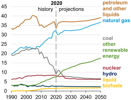
Figure 2.
Projected U.S. energy consumption showing a continued dependence on fossil fuel. Note the changes expected in the decline in coal use and rise in renewables—solar and wind, for example. (Source EIA [23]).
Two major sources of chemical reactants around cities continue to be electricity generation and transportation sectors. As the need for electricity grows to 2050, the distribution of fuels for its production is expected to change dramatically (Figure 3a). Projections for the U.S., for example, suggest coal will be supplanted more and more with natural gas and renewables.
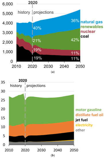
Figure 3.
Trends in fuel supply for U.S. electricity production (billion kwh) (a) and for fuels for transportation (quads) (b). Electrical generation will be dominated by natural gas through 2050; gasoline powered vehicles will continue to power most vehicles through 2050. (Source: EIA [23]).
The fuel use in the U.S. transportation sector is shown in Figure 3b. Carbon based fuel combustion is projected to continue to dominate through 2040. The contribution of electricity to this picture is expected to grow. However, it still represents a minor energy resource through 2050. The global transportation fuel resource is similar to that of the U.S. If these coarse projections remain viable today, one can estimate that for urban chemistry, energy growth relying on fossil fuels could continue to dominate reactant conditions.
2.3. Influence of Meteorology
Meteorological conditions in cities and their surroundings are widely variable on different time and space scales. Perhaps, most important to urban chemistry, are the boundary layer ambient temperature, humidity, ventilation (winds and mixing layer height) and actinometric components of solar radiation. It is known that meteorological measures vary widely daily or by season, around so-called normal (climatic) conditions. These features of weather are documented in the meteorological literature [30]. They also vary widely with geography; there are also an urban heat island and local wind flow modification (with buildings) that are well documented [31,32,33]. Example projections of urban climates were reported [34]. Long term, rapid climate changes are documented (e.g., Figure A1) A1likely to be important for urban air chemistry.
Similar to chemical processing, meteorological conditions have the potential for change over time and space ranging in scales from daily to many decades. One of the most compelling images of climate change include the long-term global temperature history shown in Figure A1. If this increase continues as an indicator of “rapid” year-by-year change, one might expect an intensification of meteorological extremes in the future. Recent research of the climate change community [35] created a hypothesis that extreme events of high temperature days and extended drought are likely to be prevalent in the future. Such changes combined with reduced humidity, cloud cover and precipitation could affect solar radiation intensity. The effect of these changes on urban air chemistry is uncertain.
Not only do meteorological constraints influence in situ chemistry, but they also affect loss or gain by air–surface exchange. Different releases or the deposition from the air surface layers modulate ambient concentrations of airborne species at rates that differ by the lability of species, surface wind, temperature and humidity [36,37,38].
The removal of chemicals from the air also involves gas and particle scavenging by precipitation. Clouds and precipitation obviously form primarily above the boundary layer, but may intermittently affect urban chemistry by the removal of species by washout or by modulating background levels [39].
3. Accounting for Chemical Change
Ambient concentrations represent a sum of in situ, ambient chemistry, air–surface chemistry, including reactants and meteorological conditions. Many of these changes have been in response to urban reactant emission reductions modified by regional conditions associated in part with the infrastructure growth of large sources outside the urban environment. Changes in the urban chemical composition have occurred since the 1950s, as measured with trends in [40,41,42,43,44]. Future change is likely to be complicated by the influence of climate change, especially on extreme events [35,45], as well as potentially radical changes in reactant emissions associated with major emission sources, e.g., energy production and use.
The inspection of the complexities of chemical interactions in the oxidant and secondary aerosol cycle (Figure 1) would suggest major uncertainties in urban conditions. Meteorological changes are expected to involve an increased frequency and intensity of temperature and humidity with drought in many locations. Solar radiation in extreme conditions of cloudiness, modulated by pollution haze, is also to be expected. Depending on the chemical species, deposition will be influenced not only by air flow and temperature, but by surface interface chemistry. Examples of such surface conditions would include the nitrogen oxides and ammonia exchange. Other cases include temperature and radiative influences on vegetation VOC emissions (e.g., isoprene, and pinenes or urban domestic vegetation species). Surface interactions with vegetation and building surfaces are likely to be a factor in chemical changes [46,47].
Perhaps most important to evolving urban chemistry will be the major changes in reactant emissions. Such changes are foreseen in source emissions, such as electricity production, which is accelerating towards major reductions in fossil fuel combustion in favor of renewables—solar and wind generation. Complementing these changes, transportation is shifting towards electric vehicles or non-fossil fuels, such as hydrogen. An example of such changes in energy production or use is shown in Figure 3. The Figure indicates that the emissions of carbon-based fuel use will decline in both electricity production and motor vehicle use, but will probably not decrease to zero in cities for the foreseeable future.
The projected changes of fossil fuel-related reactants in cities beyond these shown in the Figures could accelerate dramatically, if the current international concern for climate change results in major actions through 2050. One recent projection to cap the global temperature rise at ~1.5 °C indicated that most of the world’s fossil fuels should remain in the ground [48]. A political and technical response could move to 50% or greater solar or wind electricity in the U.S., for example. The fossil fuel reduction could also accelerate electric and other non-polluting vehicle displacements of gasoline- and diesel-fueled vehicles to >50% by 2040.
As decarbonization progresses in the energy sector, parallel emission reductions are expected in industrial emissions and in minor emissions of reactants; VOC will especially become more prevalent. These include foods for cooking and domestic use, such as cosmetic or personal use products [49]. Offsetting the reduction in anthropogenic carbon emissions is expected to major increase wildfires across the world, stimulated by extreme drought and high temperature conditions [50,51]. Wildfire smoke is observed not only locally but regionally, and continues to be a major air chemistry issue in western North America and East Asia. Wildfire emissions include not only smoke particles, but a number of indicator gases, such as NOy and O3 [52].
As noted above, workers could use at least three methods to estimate the changes in chemistry in different urban locations. These include the interpretation of historic chemical indicator trends, the interpretation of trends in terms of meteorological and emission variability, and deterministic estimates using integrated chemistry, emissions and meteorology modeling. A few examples of these approaches are discussed below.
3.1. Projecting Trends in Indicators
The long-term trends in ambient chemical indicators, such as the urban ozone, sulfur and nitrogen oxides, particle SO4 and NO3, and BC or OC, provide a chemistry baseline for projecting future conditions. The examples of ambient trends are shown in Figure 4 for the annual average concentrations of NOy, NOx, and O3 with emission trends (including VOC) for the states of Alabama, Georgia, Mississippi and northwest Florida. These data are obtained from the Southeastern Aerosol Research and Characterization Study (SEARCH) [40]. The declines include the cities of Atlanta and Birmingham. In the case shown in the Figure, there is a linear, approximately 1:1 proportional response of ambient concentrations to emission reductions, except for O3. This gas often shows a less than 1:1 proportionality to NOy, and an uncertain reduction relative to VOCs. This was observed in other locations, e.g., New York [53], as well. Across the United States, urban O3 vs. NOy trends also show proportionality [54]. In principle, the linear (or other) relationship for the ambient concentrations and reactant emissions can be adapted to project future conditions, if the emissions are the principal variation in the chemistry. Annual trends can be complemented with seasonal trends as well. For example, a shift in the seasonal O3 concentration maxima from summer towards the spring could suggest a change in chemistry.
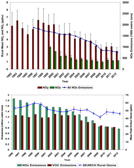
Figure 4.
Example of indicator species, NOx, NOy and the annual average O3 reductions accompanying emission reductions in southeastern U.S., including Atlanta, Georgia and Birmingham, Alabama [40].
Proportionality relationships are not necessarily forthcoming from trends between carbon sources, and OC or BC are ambiguous depending on the nature and variability of the emissions [40,55]. Analysis using forms of receptor modeling from ambient data with positive matrix factorization [56] or chemical mass balance [57] are viable alternatives, comparing apparent source groups for different years. For the complex sources of VOC and PMx, receptor modeling of the ambient data also applies. By using source identification from emission inventories, for example, ambient indicators can be associated with emissions. Blanchard et al. [55] reported such analyses for particle carbon in New York. Liu et al. [58] reviewed O3 concentration apportionment in China by analogous arguments.
The extrapolation of future conditions’ trends directly from changes in the ambient concentrations depends on the assumptions that meteorological conditions are constant on average, background concentrations have minimal variability and local source change is captured by emission inventories. These assumptions are quantitatively unlikely to be met fully in future urban conditions. Linearly proportional relationships are probably qualitatively reliable for projections in the absence of large changes in the background or spatial emission distributions.
3.2. Detailed Analysis of the Measurements
More advanced analyses of combined meteorological and ambient concentration data have the potential for the quantitative evaluation of the effects of change. Data suitable for such analyses is usually derived from specialized campaigns that generate collections well beyond air monitoring observations. These analyses come in at least two approaches. The first is an empirical study, some of which use statistical methods to associate multivariable characteristics (e.g., the application of the generalized additive model—GAM). The second derives from applicable chemical mechanisms to identify observational indexes that characterize the evolution of chemistry with ambient conditions and reactant changes in Figure 5. This analysis indicates that warming and declining RH accompany increasing O3 concentrations independent of the reactant changes.
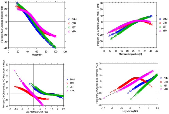
Figure 5.
Estimation of the chemistry meteorology interactions for ozone derived from the application of a generalized additive model on a large data set in southeastern U.S. BHM is Birmingham, Alabama; JST is Atlanta, Georgia; rural sites are CTR (Centreville, Alabama) and YRK (Yorkville, Georgia) [59]).
The GAM provides a means of separating inter-variable observational relationships from one another. In the case of O3 variability, one would expect both chemical and meteorological relationships for reactants, such as NOx or temperature, humidity, wind influence in the data. The sensitivity of O3 concentrations to such variables can be found in separating binary relationships from the observations, which hypothetically could be used to project future conditions with both meteorological and chemical changes.
NO concentrations tend to decrease O3. An example of a GAM analysis was reported by [59]. The authors used a large Southeastern Aerosol Research (SEARCH) data collection obtained in the southeastern U.S., including urban conditions in Atlanta, Georgia and Birmingham, Alabama. The meteorological relations with O3 were investigated using the temperature, humidity and air flow. For an indication of the independent reactant association, NOy and VOC relationships were determined. With the GAM, they were able to estimate different generalized reactant NOy to O3 and temperature humidity associations. An example of these relationships is shown in the concentrations consistent with the O3-NO titration reaction forming NO2. NO2 concentrations are associated with increasing O3 concentrations as a part of the oxidant cycle.
A second group of examples stems again from the photochemical mechanisms associated with O3 and its precursors, NOx and VOC. This series of chemical reactions to produce ozone is well known to be highly non-linear [12,60]. The non-linearity in the O3 chemistry was shown in an ambient (morning) VOC-NOx vs. O3 concentration isopleth plot emphasizing the significance of the VOC/NOx ratio in O3 production. Ozone in many cities was initially identified with a so-called VOC sensitive regime, but more recently most urban areas have shifted to a NOx sensitive regime for the chemistry. These “sensitivity” relationships for O3 change have been investigated extensively since the 1960s [11,12].
Another example of the second method concerns O3 and O3 production efficiency (OPE); the latter is the change in O3 with change in NOy or NOz. Theoretically, the OPE should increase with lower NOy concentrations, so that O3 concentration, decreased from NOx reductions, should be offset with the increase in O3 production [61]. The rise in OPE with declines in NOy or NOz was observed in the Southeast and in the New York area [62,63]. An example for the southeastern area of the U.S. is indicated in Figure 6.
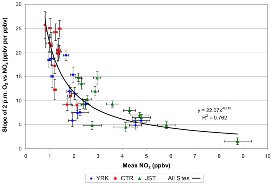
Figure 6.
Variation of a measure of O3 production efficiency with NOz. JST is an urban site in Atlanta, YRK is a suburban Atlanta site, and CTR (Centreville) is a rural remote site. Urban conditions reflect relatively low OPE, while rural cases show much higher OPE, tending to offset the effect of ozone concentrations with NOy. (From Blanchard and Hidy [62]).
The OPE results complement other projections that establish theoretically and observationally the relationship between O3 as a photochemical indicator and reactant concentrations of VOC and NOx. This implies that O3 response to NOx reductions from switching to non-fossil fuel vehicles will be offset by increasing OPE not only regionally, but within cities
3.3. Projections from Ambient Air Modeling
The third alternative for the exploration of urban chemistry with change uses air chemical transport modeling. This deterministic approach integrates chemistry, meteorology and emissions over a broad range of spatial and temporal scales [64,65]. Similar to all practical models of atmospheric phenomena, these models involve approximations for each of the major elements. The chemistry module involves an approximate mechanism based on extensive and detailed analyses for gas phase processes and less well-established mechanisms supported by laboratory experiments of kinetics and simulation chambers [66]. The emissions for urban areas are an approximation based on annual or short-term inventories spatially and temporally for gases and particles. In principle, the meteorological component can be estimated using a separate model that calculates winds, temperature, humidity and solar radiation [64,65,67]. The model results are “calibrated” for a given year or shorter interval using ambient data and meteorological observations.
The applications and sensitivity of the model predictions can be evaluated for chemistry, meteorology and emissions assuming changes in past conditions and expected in the future. Examples of such studies include (a) the intercomparison of truncated chemical reaction mechanisms [34,68,69]; (b) the investigation of “sudden” emission reduction (e.g., the COVID-19 experience [70,71]); (c) the influence on urban air chemistry considering the meteorology of “the street canyon effect” [72]; (d) the sensitivity to climate conditions [73]; and (e) projections of urban- or city-specific O3 trends to 2100 varying O3 background [74,75]. Each of these computer-based experiments add insight into gas phase and in some cases particle chemistry in the light of meteorological and emission-deposition conditions.
Chemical mechanisms can also be explored in detail using simpler models, such as a “traveling” box model. An example of this approach that extends a detailed gas phase model to heterogeneous reactions was reported [76].
4. Discussion and Conclusions
The end products of gas and condensed phase chemistry of urban atmospheres are the result of various ambient processes that include not only chemical mechanisms with reactants entering the air [77], but also reactant product losses at the ground and meteorological influences. The average ambient concentrations change in time and space. Through most of the 20th and early 21st centuries, these changes are seen within normal or forecasted meteorology, while focusing mainly on the gradual changes in reactant emissions. Ambient chemical processing has changed conceptually as new knowledge of oxidant photochemistry and aerosol formation has emerged from the 1950s and beyond.
In the future, urban chemistry is anticipated to continue changing in potentially more dramatic ways with major shifts in emissions, partly associated with reductions in the energy and transportation sectors taking place along with urban demography. Changes in emissions in part will depend significantly on the social and ecological impact of climate warming. Urban chemistry will also depend on the meteorological conditions [78] involving extreme events as well as average temperature and humidity changes, and the potential for the modulation of solar radiation by clouds and haze.
The evolution of urban air chemistry for future conditions can be inferred to an extent with response to forcing that has occurred in the past. Approaches to such inferences are suggested that range from the simple comparison of trends in ambient composition with reactant emissions to advanced deterministic modeling integrating chemical mechanisms with reactant input, meteorological conditions and deposition in cities. These methods have limitations, but in combination present an insight into the future with major demographic changes in cities. Across the world, urban environments are culturally and technologically distinct. However, in most cities, the common denominators for major reactant emissions are energy production and use, particularly in the transportation sector. These two sources of reactants are likely to dominate local gas phase and aerosol chemistry.
Given the projections of energy production and use for the next decades, exemplified in Figure 2 and Figure 3, in the aggregate it would seem that fossil fuels will continue to dominate the urban reactant emissions. Individual cities may have modified emissions from industry and commercial activity, but it is likely that the current picture of photochemistry-dominated air will prevail for some time. The same cannot be necessarily said for aerosols. Particle composition and chemistry in urban air will shift more towards the dominance of carbon species, with relatively large uncertainty in the production of known or unidentified species appearing. The hypothetical “guesses” about the change observed in gas and aerosol chemistry, in Table 1 and Table 2, are the expectations of indicator change based on the dominance of fossil fuels in cities. The listed indicators may be too coarse to observe the subtle changes in chemistry. Greater attention to species of a higher sensitivity to change will probably be needed to document future chemical processing.
Urban chemistry can also no longer be separated from regional activity, or even intra or intercontinental conditions. Accounting or local processes imbedded in a “background” of chemicals is especially important to aerosols, where urban conditions depend on a multiscale mix of primary and secondary particles from air transport, not in the least of which are wildfire smoke. Smoke and haze have been agents of change in urban carbon chemistry in the last few years, and are expected to continue to be the keys to urban chemistry in the future.
Funding
This research received no external funding.
Conflicts of Interest
The authors declare no conflict of interest.
Appendix A

Figure A1.
Change in the global mean temperature (1880–2020). Note that the graph emphasizes the rapid warming at the surface relative to the 1970s, suggesting a continued sharp increase in the near future. (Graph courtesy of NASA).
Table A1.
Reactant or product indicators for urban chemistry for major cities. H = High concentrations exceeding WHO regulatory air pollution guidelines by more than 2×; M = Moderate concentrations exceeding WHO guidelines by less than 2×; L = low WHO guidelines generally met; and -- Inadequate data. (Based on tabulations from Harrington and McConnell [79]).
| City | Population a | CO | SO2 | NOx | O3 | TSP b | Lead |
|---|---|---|---|---|---|---|---|
| Bangkok | 10.3 | L | L | L | L | H | M |
| Beijing | 11.5 | - | H | L | M | H | L |
| Buenos Aires | 13.0 | - | - | - | - | M | L |
| Cairo | 11.8 | M | - | - | - | H | H |
| Calcutta | 15.9 | - | L | L | - | H | L |
| Jakarta | 13.2 | M | L | L | M | H | M |
| London | 10.8 | M | L | L | L | L | L |
| Los Angeles | 10.9 | M | L | M | H | M | L |
| Manila | 11.5 | - | L | - | - | H | M |
| Mexico City | 24.4 | H | H | M | H | H | M |
| Moscow | 10.1 | M | - | M | -- | M | L |
| New York | 16.1 | M | L | L | M | L | L |
| Rio de Janeiro | 13.0 | L | M | - | - | M | L |
| Seoul | 13.0 | L | H | L | L | H | L |
| Shanghai | 14.7 | - | M | - | - | H | - |
| Tokyo | 21.3 | L | L | L | H | L | – |
a Estimated in 2000 (millions). b Total suspended particles, diameter < 35 μm. Source contributions from primary sources and atmospheric reactions of S, N and C.
Table A2.
Illustration of motor vehicle contribution (% of emissions) to reactants in cities. (Based on tabulations from [79]).
Table A2.
Illustration of motor vehicle contribution (% of emissions) to reactants in cities. (Based on tabulations from [79]).
| By Country | CO | SO2 | NOx | NMHC | TSP |
|---|---|---|---|---|---|
| United States | 66 | - | 43 | 48 a | - b |
| Germany | 74 | 6 | 65 | 53 a | - |
| United Kingdom | 86 | 2 | 49 | 32 a | - |
| By City | |||||
| Budapest | 81 | 12 | 57 | 75 | - |
| Cochin (India) | 70 | - | 77 | 95 | - |
| Delhi | 90 | 13 | 59 | 85 | 37 |
| Lagos | 91 | 27 | 62 | 20 | 69 |
| Mexico City | 97 | 22 | 75 | 53 | 35 |
| Santiago | 95 | 14 | 85 | 69 | 11 |
| Sao Paulo | 94 | 64 | 92 | 89 | 39 |
a Value is for VOC; NMHC is a portion of VOC. b PM2.5, a fraction of TSP is estimated for U.S. cities ~30% (mostly carbon, sulfate and nitrate).
References
- Smith, R.A. Air and Rain; Longmans, Green & Co., Ltd.: London, UK, 1872. [Google Scholar]
- Bojkov, R.D. Surface Ozone during the Second Half of the Nineteenth Century. J. Clim. Appl. Meteorol. 1986, 25, 343–352. [Google Scholar] [CrossRef]
- Aitken, J. Collection of Scientific Papers; Cambridge University Press: London, UK, 1923. [Google Scholar]
- Landsburg, H. Atmospheric Condensation Nuclei. Ergeb. Kosm. Phys. 1938, 3, 155–222. [Google Scholar]
- Brimblecombe, P. The Big Smoke; Methuen: London, UK, 1987. [Google Scholar]
- Harrison, R. Urban atmospheric chemistry: A very special case for study. NPJ Clim. Atmos. Sci. 2018, 1, 20175. [Google Scholar] [CrossRef]
- Schrenk, H.; Hieman, H.; Clayton, G.; Gafafer, W.; Wexler, H. Air Pollution in Donora, Pa; Bull. 306; U.S. Public Health Service: Washington, DC, USA, 1949.
- Haagen Smit, A.; Bradley, C.; Fox, M. Ozone Formation in Photochemical Oxidation of Organic Substances. Ind. Eng. Chem. 1953, 45, 2086–2089. [Google Scholar] [CrossRef]
- Stern, A. History of Air pollution Legislation in the United States. J. Air Poll. Contr. Assoc. 1982, 32, 44–61. [Google Scholar] [CrossRef] [PubMed]
- U.S. Congress. The Air Quality Act of 1967; U.S. Public Law 90–148; U.S. Government: Washington, DC, USA, 1967.
- Leighton, P. Photochemistry of Air Pollution; Academic Press: New York, NY, USA, 1961. [Google Scholar]
- Finlayson-Pitts, B.; Pitts, J., Jr. Chemistry of the Upper and Lower Atmosphere; Academic Press: New York, NY, USA, 2000. [Google Scholar]
- Seinfeld, J.; Pandis, S. Atmospheric Chemistry and Physics; John and Wiley and Sons: New York, NY, USA, 2006. [Google Scholar]
- Hallquist, M.; Wenger, J.C.; Baltensperger, U.; Rudich, Y.; Simpson, D.; Claeys, M.; Dommen, J.; Donahue, N.M.; George, C.; Goldstein, A.H.; et al. The formation, properties and impact of secondary organic aerosol: Current and emerging issues. Atmos. Chem. Phys. 2009, 9, 3555–3762. [Google Scholar] [CrossRef]
- Carlton, A.; Wiedinmyer, C.; Kroll, J. A review of Secondary Organic Aerosol (SOA) formation from isoprene. Atmos. Chem. Phys. 2009, 9, 4987–5005. [Google Scholar] [CrossRef]
- Hidy, G.; Blanchard, C. The North American background aerosol and global aerosol variation. J. Air Waste Manag. Assoc. 2005, 55, 1585–1599. [Google Scholar] [CrossRef]
- Congressional Research Service. Background Ozone: Challenges in Science and Policy. R45482. 2019. Available online: https://sgp.fas.org/crs/misc/R45482.pdf (accessed on 15 August 2021).
- Jamriska, M.; Dubois, T.; Skvortsov, A. Statistical characterization of bio-aerosol background in an urban environment. Atmos. Environ. 2012, 54, 439–448. [Google Scholar] [CrossRef]
- Roiger, A.; Huntreiser, H.; Schlager, H. Long range transport of air pollutants. In Atmospheric Physics; Schumann, U., Ed.; Springer: Berlin/Heidelberg, Germany, 2012. [Google Scholar] [CrossRef]
- Qian, W.; Quan, L.; Shi, S. Variations of the Dust Storms in China and its Climate Control. J. Clim. 2002, 15, 1216–1229. [Google Scholar] [CrossRef]
- Wikipedia. Wildfires in 2021. Available online: https://en.wikipedia.org/wiki/Wildfires_in_2021 (accessed on 15 December 2021).
- McMurry, P.; Shepherd, M.; Vickery, J. (Eds.) Particulate Matter Science for Policy Makers; Cambridge University Press: Cambridge, UK, 2004. [Google Scholar]
- U.S. Energy Information Administration. Annual Energy Outlook 2021. Available online: https://www.google.com.hk/url?sa=t&rct=j&q=&esrc=s&source=web&cd=&cad=rja&uact=8&ved=2ahUKEwjlsKPPo4H2AhX1slYBHcxnD6AQFnoECAkQAQ&url=https%3A%2F%2Fnangs.org%2Fanalytics%2Fdownload%2F6477_98746e3569d4350e2f00a2011814083d&usg=AOvVaw3xFY5ZKkRxzenKd8J3XKP6 (accessed on 30 September 2021).
- Carter, W. Development of ozone reactivity scales for volatile organic compounds. J. Air Waste Manag. Assoc. 1994, 44, 881–899. [Google Scholar] [CrossRef]
- U.S. Environmental Protection Agency. 2020 National Emissions Inventory (NEI). Available online: https://www.healthypeople.gov/2020/data-source/national-emissions-inventory (accessed on 2 September 2021).
- Henneman, L.; Shen, H.; Hogrefe, C.; Russell, A.; Zigler, M. Four decades of United States Mobile Source Pollutants: Spatial-Temporal Trends Assessed by Ground-Based Monitors, Air Quality Models, and Satellites. Environ. Sci. Technol. 2021, 55, 882–892. [Google Scholar] [CrossRef]
- U.S. Environmental Protection Agency. 2017 National Emission Inventory Based Photochemical Modeling for Sector Specific Air Quality Assessments; Office of Air Quality Planning and Standards: Research Triangle Park, NC, USA, 2017.
- Miller, C.A.; Hidy, G.; Hales, J.; Kolb, C.E.; Werner, A.S.; Haneke, B.; Parrish, D.; Frey, H.C.; Rojas-Bracho, L.; DesLauriers, M.; et al. Air emission inventories in North America: A Critical Assessment. J. Air Waste Manag. Assoc. 2006, 56, 1115–1129. [Google Scholar] [CrossRef]
- U.S. Energy Information Administration. International Energy Outlook 2021; Energy Information Administration: Washington, DC, USA, 2021. Available online: https://www.eia.gov/outlooks/ieo/ (accessed on 8 October 2021).
- Carlson, T. Mid-Latitude Weather Systems; American Meteorological Society: Boston, MA, USA, 1998. [Google Scholar]
- Hicks, B.; Novakovskia, E.; Dobosy, R.; Pendergrass, W., III. Temporal and spatial aspects of velocity variance in the urban surface roughness layer. J. Appl. Meteorol. Climatol. 2013, 52, 668–681. [Google Scholar] [CrossRef]
- U.S. Environmental Protection Agency. Heat Island Effect. Available online: https://www.epa.gov/heatislands (accessed on 2 September 2021).
- Barlow, J. Progress in observing and modeling the urban boundary layer. Urban Clim. 2014, 10, 216–240. [Google Scholar] [CrossRef]
- Zhao, L.; Oleson, K.; Bou-Zeid, E.; Krayenhoff, E.S.; Bray, A.; Zhu, Q.; Zheng, Z.; Chen, C.; Oppenheimer, M. Global multi-model projections of local urban climates. Nat. Clim. Chang. 2021, 11, 152–157. [Google Scholar] [CrossRef]
- National Academy of Sciences. Attribution of Extreme Weather Events in the Context of Climate Change; The National Academies Press: Washington, DC, USA, 2016. [Google Scholar]
- Wesley, M.; Hicks, B. A review of the current status of knowledge on dry deposition. Atmos. Environ. 2000, 34, 2260–2282. [Google Scholar] [CrossRef]
- Decina, S.; Hutyra, L.; Templer, P. Hotspots of nitrogen deposition in the world’s urban areas: A global data synthesis. Front. Ecol. Environ. 2020, 18, 92–100. [Google Scholar] [CrossRef]
- Lohse, K.; Hope, D.; Sponseller, R.; Allen, J.; Grimm, M. Atmospheric deposition of carbon and nutrients across an arid metropolitan area. Sci. Total Environ. 2008, 402, 95–105. [Google Scholar] [CrossRef]
- Irving, P. (Ed.) Acidic Deposition: State of Science and Technology. Precipitation Scavenging; U.S. National Acid Precipitation Program: Washington, DC, USA, 1991; Volume 1, pp. 109–168.
- Hidy, G.M.; Blanchard, C.L.; Baumann, K.; Edgerton, E.; Tanenbaum, S.; Shaw, S.; Knipping, E.; Tombach, I.; Jansen, J.; Walters, J. Chemical Climatology of the southeastern United States, 1999–2013. Atmos. Chem. Phys. 2014, 14, 11893–11914. [Google Scholar] [CrossRef]
- Yan, Y.; Pozzer, A.; Ojha, N.; Lin, J.; Lelieveld, J. Analysis of European ozone trends in the period 1995–2014. Atmos. Chem. Phys. 2018, 18, 5589–5605. [Google Scholar] [CrossRef]
- Xing, J.; Mathur, R.; Pleim, J.; Hogrefe, C.; Gan, C.M.; Wong, D.C.; Wei, C.; Wang, J. Air pollution and climate response to aerosol direct radiative effects: A modeling study of decadal trends across the northern hemisphere. J. Geophys. Res. Atmos. 2015, 120, 12–221. [Google Scholar] [CrossRef]
- Akiyoshi, I.; Wakamatsu, S.; Morikawa, T.; Kobayashi, S. 30 Years of Air Quality Trends in Japan. Atmosphere 2021, 12, 1072. [Google Scholar] [CrossRef]
- Mou, Y.; Song, Y.; Xu, Q.; He, Q.; Hu, A. Influence of Urban-Growth on Air Quality in China: A Study of 338 Cities. Int. J. Res. Public Health 2018, 15, 1805. [Google Scholar] [CrossRef] [PubMed]
- Hong, C.; Zhang, Q.; Zhang, Y.; Davis, S.J.; Tong, D.; Zheng, Y.; Liu, Z.; Guan, D.; He, K.; Schellnhuber, H.J. Impacts of climate change on future air quality and human health in China. Proc. Natl. Acad. Sci. USA 2019, 116, 17193–17200. [Google Scholar] [CrossRef] [PubMed]
- Nowak, D.; Civerolo, K.; Rao, S.; Sistla, G.; Ouley, C.; Crane, D.A. Modeling study of the impact of urban trees on ozone. Atmos. Environ. 2000, 34, 1601–1613. [Google Scholar] [CrossRef]
- Fitzky, A.C.; Sandén, H.; Karl, T.; Fares, S.; Calfapietra, C.; Grote, R.; Saunier, A.; Rewald, B. The Interplay between Ozone and Urban Vegetation—BVOC Emission, Ozone Deposition and Tree Ecophysiology. Front. For. Glob. Chang. 2019, 2, 50. [Google Scholar] [CrossRef]
- Welsby, D.; Price, J.; Ekins, P. Unextractable fossil fuels in a 1.5 °C world. Nature 2021, 597, 230–324. [Google Scholar] [CrossRef]
- Lewis, A. The changing face of urban air pollution: Volatile organic compounds in the U.S. urban air increasingly derive from consumer products. Science 2018, 359, 744–745. [Google Scholar] [CrossRef]
- Jaffe, D.A.; O’Neill, S.M.; Larkin, N.K.; Holder, A.L.; Peterson, D.L.; Halofsky, J.E.; Rappold, A.G. Wildfire and prescribed burning impacts on air quality in the United States. J. Air Waste Manag. Assoc. 2020, 70, 583–615. [Google Scholar] [CrossRef]
- Chen, J.; Li, C.; Ristovski, Z.; Milic, A.; Gu, Y.; Islam, M.S.; Wang, S.; Hao, J.; Zhang, H.; He, C.; et al. A review of biomass burning: Emissions and impacts on air quality and climate in China. Sci. Tot. Environ. 2017, 579, 1000–1034. [Google Scholar] [CrossRef]
- Urbanski, S.; Hap, W.; Baker, S. Chemical composition of wildland fire emissions. In Developments in Environmental Science; Bytneroweiz, A., Arbaugh, M., Andersen, C., Riebau, A., Eds.; Elsevier: London, UK, 2009; Volume 8, Chapter 4. [Google Scholar]
- Blanchard, C.; Shaw, S.; Edgerton, E.; Schwab, J. Emission influences on air pollutant concentrations in New York State: I. ozone. Atmos. Environ. 2019, 3, 100033. [Google Scholar] [CrossRef]
- Hidy, G.M.; Blanchard, C.L. Precursor reductions and ground-level ozone in the continental United States. J. Air Waste Manag. Assoc. 2015, 65, 1261–1282. [Google Scholar] [CrossRef]
- Blanchard, C.; Shaw, S.; Edgerton, E.; Schwab, J. Ambient PM2.5 organic and elemental carbon in New York City: Changing source contributions during a decade of large emission reductions. J. Air Waste Manag. Assoc. 2021, 71, 995–1012. [Google Scholar] [CrossRef]
- Hopke, P.; Dai, Q.; Li, L.; Feng, Y. Global review of recent source apportionments for airborne particulate matter. Sci. Tot. Environ. 2020, 740, 140091. [Google Scholar] [CrossRef]
- U.S. Environmental Protection Agency. Chemical Mass Balance Model. Available online: www.epa.gov/scram/chemical-mass-balance-cmb-model (accessed on 28 September 2021).
- Liu, H.; Zhang, M.; Ham, X. A review of surface ozone source apportionment in China. Atmos. Ocean. Sci. Let. 2020, 13, 470–484. [Google Scholar] [CrossRef]
- Blanchard, C.; Hidy, G. Ozone in the Southeastern United States: An Observationally-Based Model Using Measurements from the SEARCH Network. Atmos. Environ. 2014, 48, 192–200. [Google Scholar] [CrossRef]
- National Research Council. Rethinking the Ozone Problem in Urban and Regional Air Pollution; National Academy Press: Washington, DC, USA, 1991. [Google Scholar]
- Lin, X.; Trainer, M.; Liu, S.C. On the nonlinearity of the tropospheric ozone production. J. Geophys. Res. Atmos. 1988, 93, 15879–15888. [Google Scholar] [CrossRef]
- Blanchard, C.; Hidy, G. Ozone Response to Emission Reductions in the Southeastern United States. Atmos. Chem. Phys. 2018, 18, 8183–8202. [Google Scholar] [CrossRef]
- Ninneman, M.; Demerjian, K.; Schwab, J. Ozone Production Efficiencies at Rural New York State Locations: Relationship to Oxides of Nitrogen Concentrations. J. Geophy. Res. Atmos. 2019, 124, 2363–2376. [Google Scholar] [CrossRef]
- Kim, Y.; Wu, Y.; Seigneur, C.; Roustan, Y. Multi-scale modeling of urban air pollution: Development and application of a Street-in-Grid model (v1.0) by coupling MUNICH (v1.0) and Polair3D (v1.8.1). J. Geosci. Model Dev. 2018, 11, 611–629. [Google Scholar] [CrossRef]
- Mailler, S.; Menut, L.; Khvorostyanov, D.; Valari, M.; Couvidat, F.; Siour, G.; Turquety, S.; Briant, R.; Tuccella, P.; Bessagnet, B.; et al. CHIMERE_2017: From urban to hemispheric chemistry-transport modeling. J. Geosci. Model Dev. 2017, 10, 2397–24223. [Google Scholar] [CrossRef]
- Carter, W. Development of a Condensed SAPRAC-07 Chemical Mechanism. Atmos. Environ. 2010, 44, 5336–5345. [Google Scholar] [CrossRef]
- U.S. Environmental Protection Agency. The Community Multiscale Air Quality Modeling System. Available online: www.epa.gov/cmaq (accessed on 4 September 2021).
- Yu, S.; Sawar, G.; Kang, D.; Tong, D.; Pouliot, G.; Pleim, J.; Mathur, R. CMAQ air quality forecasts for O3 and related species using three different photochemical mechanisms (CBS, CB05, SAPRC-99): Comparison with measurements during the 2004 ICARTT study. Atmos. Chem. Phys. 2010, 10, 3001–3025. [Google Scholar] [CrossRef]
- Jiminez, P.; Baldasano, J.; Dabdub, D. Comparison of photochemical mechanisms for air quality modeling. Atmos. Environ. 2003, 37, 4179–4194. [Google Scholar] [CrossRef]
- Deroubaix, A.; Brasseur, G.; Gaubert, B.; Labuhn, I.; Menut, L.; Siour, G.; Tuccella, P. Response of surface ozone concentration to emission reduction and meteorology during the COVID-19 lockdown in Europe. Meteorol. Appl. 2021, 28, e1990. [Google Scholar] [CrossRef]
- Yang, J.; Wen, Y.; Wang, Y.; Zhang, S.; Pinto, J.P.; Pennington, E.A.; Wang, Z.; Wu, Y.; Sander, S.P.; Jiang, J.H.; et al. From COVID-19 to future electrification: Assessing traffic impacts on air quality by a machine-learning model. Proc. Natl. Acad. Sci. USA 2021, 118, e2102705118. [Google Scholar] [CrossRef]
- Kim, M.; Park, R.; Kim, J. Urban air quality modeling with full O3-NOx-VOC chemistry: Implications for O3 and PM air Quality in a street canyon. Atmos. Environ. 2012, 47, 330–340. [Google Scholar] [CrossRef]
- Dawson, J.; Adams, P.; Pandis, S. Sensitivity of ozone to summertime climate in the eastern USA: A modeling case study. Atmos. Environ. 2007, 41, 1494–1511. [Google Scholar] [CrossRef]
- Colette, A.; Granier, C.; Hodnebrog, O.; Jakobs, H.; Maurizi, A.; Nyiri, A.; Bessagnet, B.; D’Angiola, A.; D’Isidoro, M.; Gauss, M.; et al. Air Quality Trends in Europe over the Past Decade: A first Multi-Model Assessment. Atmos. Chem. Phys. 2012, 12, 11657–11678. [Google Scholar] [CrossRef]
- Royal Society. Ground-Level Ozone in the 21st Century: Future Trends, Impacts and Policy Implications; Report 15/08; Royal Society: London, UK, 2008. [Google Scholar]
- Springmann, M.; Knopf, D.; Riemer, N. Detailed heterogeneous chemistry in an urban plume box model: Reversible co-adsorption of O3, NO2 and H2O on soot coated with benzo[a]pyrene. Atmos. Chem. Phys. 2009, 9, 7461–7479. [Google Scholar] [CrossRef]
- Archibald, A.; Turnock, S.; Griffiths, P.; Cox, T.; Dent, R.; Kbnote, C.; Shin, M. On the changes in surface ozone over the 21st century: Sensitivity to changes in surface temperature and chemical mechanisms. Phil. Trans. R. Soc. A 2020, 378, 20190329. [Google Scholar] [CrossRef]
- Austin, E.; Zanobetti, A.; Coull, B.; Schwartz, J.; Gold, D.; Koutrakis, P. Ozone trends and their relationship to characteristic weather patterns. J. Expo. Sci. Environ. Epidemiol. 2015, 25, 532–542. [Google Scholar] [CrossRef]
- Harrington, W.; McConnell, V. Motor Vehicles and the Environment; Resources for the Future: Washington, DC, USA, 2003. [Google Scholar]
Publisher’s Note: MDPI stays neutral with regard to jurisdictional claims in published maps and institutional affiliations. |
© 2022 by the author. Licensee MDPI, Basel, Switzerland. This article is an open access article distributed under the terms and conditions of the Creative Commons Attribution (CC BY) license (https://creativecommons.org/licenses/by/4.0/).