Derivation of High-Resolution Meteorological Parameters for Use in Airport Wind Shear Now-Casting Applications

Abstract

Methods for now-casting adverse weather conditions with the potential to cause disruption to aircraft landings often make use of real-time measurements at high temporal resolution. This paper describes processing methodologies developed to derive meteorological parameters from such measurements recorded in the vicinity of Hong Kong International Airport, specifically a radiometer in King’s Park, a wind profiler and surface anemometer on Cheung Chau Island and weather buoys in the Pearl River estuary. These parameters are suitable for use as input to a now-casting application of the computationally efficient airflow model, FLOWSTAR, which has previously been shown to predict mountain waves generated by flow over Lantau Island to the southeast of the airport. Radiosonde data from King’s Park have been used to test the radiometer processing method; the novel approach of using minimum and maximum potential temperature deviations from a series of height-dependent linear profiles to derive radiometer inversion layer parameters generates data that compares well with values derived from corresponding radiosonde profiles. Mountain wave strength depends on the magnitude of wind speed in the inversion layer; wind profiler data can be used to estimate typical and maximum wind speeds and associated wind directions using estimates of inversion layer depth derived from the radiometer data. With estimates of surface sensible heat flux appropriate for the airport’s coastal location calculated using a marine boundary layer scheme, a dataset of meteorological parameters at 20-min resolution has been derived for input into the FLOWSTAR model. The combination of automated meteorological data processing methods and flow field modelling has the potential to form part of a now-casting system for determining strong wind shear conditions at the airport.

1. Introduction

Aircraft landing at airports located in the vicinity of significantly elevated terrain may experience less than ideal meteorological conditions due to the influence of mountains on air flow and turbulence. Aircraft landings at Hong Kong International Airport (HKIA) have been subject to episodes of significant wind shear and turbulence since opening in 1998 [1]; HKIA is located on reclaimed land to the northwest of Lantau Island, which has a maximum elevation of nearly 1000 m. There are many other airports which experience similar problems, such as the island of St Helena in the South Atlantic, where landings have been disrupted due to turbulence generated by the elevated terrain to the northeast of the airport [2], as well as Bodo (Norway), Punta Arenas (Chile), Comodoro Rivadavia (Argentina) and Dutch Harbor (Alaska).

If pilots have advance warning of adverse conditions, with the assistance of air traffic control personnel, appropriate action can be taken to avoid dangerous landings, for instance, use of alternative runways or airports [2]. Such warning systems can be developed through application of a variety of methods, such as deployment of instrumentation near the airport [3] or use of numerical weather prediction (NWP) models to calculate flow and turbulence fields [4]; systems may use a combination of both of these approaches [5]. Alternative solutions to similar complex, non-linear problems involving multiple variables may be found through the application of machine learning, for instance, using neural networks to optimize aerodynamic parameters in relation to unmanned aerial vehicles [6].

Some NWP models configured to represent current weather conditions at airports require real-time meteorological measurements as input. One accurate source of meteorological measurement data is radiosonde soundings, but these are only taken 6- or 12-hourly, so have insufficiently high temporal resolution for use as input to a now-casting system. Radiosonde data are, however, useful for assessing the accuracy of other higher temporal resolution datasets.

Multiple high-temporal resolution measurement instruments have been deployed by the Hong Kong Observatory in the vicinity of HKIA and on the mainland at King’s Park (Yau Tsim Mong) that can assist with identifying adverse weather conditions, specifically surface anemometers, wind profilers, weather buoys, a light detection and ranging (LiDAR) instrument and a microwave radiometer. Studies have been undertaken reviewing the measurement datasets recorded by these instruments and in some cases, additionally data from equipment onboard aircraft. Inter-comparisons of measurements taken using different equipment are presented in the literature, in addition to comparisons of measurements against numerical weather prediction (NWP) model data. A detailed description of HKIA weather buoy stations has been published [7], with the aim of using the data for wind shear estimation, and comparisons of LiDAR scans against meteorological measurements recorded by surface anemometers and weather buoys have been undertaken [8]. A particular wind shear episode has been investigated by looking at LiDAR, on-board records and NWP data [9], and vortex/wave shedding in the vicinity of HKIA during an event in 2014 has been studied, making use of surface anemometer and wind profiler measurements for evaluating NWP model performance [10]. LiDAR and weather buoy observations have been used to evaluate high-resolution NWP model performance for particular adverse conditions [4], and the same system was further evaluated for a two-year period by comparison with pilot wind shear reports in [11]. A methodology for the use of anemometer, LiDAR and microwave radar data in operational wind shear algorithms has been developed [3]. In addition to these literature studies, Hong Kong Observatory publishes accessible information on wind shear and turbulence for pilots and air navigators, including details of the Hong Kong aviation weather alerting service [12].

Mesoscale NWP models such as the Weather Research and Forecasting (WRF) model developed by the US National Centre for Atmospheric Research (NCAR) can be applied at a range of scales, from tens of meters to thousands of km. When run at fine resolution, the model can be used to capture terrain-disrupted airflow. Hong Kong Observatory (HKO) have developed a system incorporating WRF that resolves air flow at 200 m resolution in the vicinity of HKIA [4]; the system has been shown to capture complex air flow features that occur in this region, specifically foehn winds [13] and mountain waves [14].

The FLOWSTAR model [15] is a quasi-linear, steady state perturbation model which characterizes the atmosphere using up to three layers comprising a boundary layer, where, near the surface, account is taken of the impact of upwind shear and locally generated turbulence on the perturbations in mean flow; an elevated inversion layer; and a stable layer aloft where the terrain may generate both propagating and trapped internal gravity waves. By configuring FLOWSTAR with terrain and meteorological datasets corresponding to the topography and atmospheric conditions in the vicinity of HKIA, it has been possible to broadly reproduce the large-amplitude mountain waves generated by air masses passing over Lantau Island that can lead to wind shear conditions at the airport [16,17,18]. Specific meteorological conditions lead to mountain waves, namely, a combination of high wind speeds, a strong low-level elevated inversion with a large temperature jump and relatively low buoyancy frequency at the top of the inversion. In order for the FLOWSTAR model to form part of a wind shear now-casting system, real-time estimates of a number of inversion-layer parameters are required: height, wind speed (typical/maximum), wind direction and temperature jump. In addition, the model requires an estimate of the surface sensible heat flux, the buoyancy frequency above the inversion layer and a representative wind direction profile, the latter required because the core model only allows for one input wind direction. The purpose of this paper is twofold. Firstly, following identification of suitable measurement instruments, processing methodologies that allow generation of the required FLOWSTAR input parameters are presented. Secondly, the accuracy of the wind- and temperature-related, high-resolution datasets is evaluated using more precise radiosonde data; other evaluation techniques are presented for the surface sensible heat flux parameter.

The aim of the current work is not only to derive meteorological parameters suitable for use in a now-casting system but also to apply an initial filtering of the meteorological data into time periods that are more (or less) likely to lead to adverse conditions at HKIA. This is problematic because mountain waves are not the only cause of adverse weather conditions at the airport: strong wind veering and combinations of other wind/atmospheric conditions prevalent in mountainous regions may also generate sharp headwind changes [19]. For the current study, the meteorological data are filtered for cases where the FLOWSTAR model may predict mountain waves.

The methods section reviews meteorological measurement data availability in the vicinity of the airport. Meteorological processing methods are then presented, separately for the radiometer, wind profiler/anemometer and weather buoys. Key outcomes of the evaluation of the derived datasets are then given. The paper concludes with a discussion of the relative merits of the processing techniques developed, the evaluation results and recommendations for improvements to the current approach.

2. Methods

Meteorological measurement availability is presented in Section 2.1, and meteorological processing methods are described in Section 2.2. Where informative, data examples from the period January to April 2019 are presented; more comprehensive results from the processing of measurements for this period are presented in the results section.

2.1. Meteorological Measurement Availability

HKO has a network of instruments that record meteorological data over the Hong Kong Special Administrative Region (HKSAR). The majority of the instruments are automatic, recording meteorological parameters at high temporal resolution; details of the instrument type, location height and parameters measured are given in [20]. Figure 1 shows the domain over which the measurement instrumentation relevant to this study has been deployed. King’s Park (KP) in Kowloon is the site for the radiometer; wind profiler data and surface anemometer data are taken from Cheung Chau Island (CCH) to the southeast of Lantau Island; sea surface temperature and air temperature are taken from weather buoys 1 and 4 (WB1, WB4) close to the airport. In addition to the mountainous terrain, the marine environment also influences meteorological conditions at the airport; Figure 1 shows HKIA in relation to the Pearl River estuary, which is of relevance to the surface sensible heat flux calculations. The HKIA northern and southern runways are shown for reference.

A number of meteorological parameters are required as input to the FLOWSTAR model. Specifically, the strength of the temperature inversion, the wind speed in the inversion layer, the buoyancy frequency above the inversion layer and the inversion layer height are the dominating meteorological parameters that influence the generation of mountain waves at HKIA; atmospheric stability in the boundary layer is also important, and a wind direction vertical profile is required in order to re-combine multiple FLOWSTAR model outputs, as the core model only allows for one input wind direction. In previous work, these parameters were derived from archived meteorological datasets recorded in the vicinity of HKIA but for a now-casting application, real-time data model inputs are required.

Table 1. Summary of data sources for meteorological parameters required as input to the FLOWSTAR model: comparison of hindcasting and now-casting data.

Parameter	Previous Modelling (Hindcasting)	Current Calculation (Now-Casting)
Boundary layer height	Radiosonde temperature data	Real-time radiometer data
Potential temperature jump in the inversion layer
Buoyancy frequency at the top of the boundary layer
Wind speed and direction in the inversion layer	Radiosonde wind data and archived wind profiler data from CCH	Real-time wind profiler data
Wind direction vertical profile in the boundary layer	Radiosonde wind data	Real-time wind profiler data and surface anemometer data from CCH
Surface sensible heat flux	Assumed zero	Real-time sea temperature, air temperature and wind speed data from a weather buoy to the east of HKIA

compares the meteorological parameter data sources used for previous hindcasting applications [16,17,18] and for the current now-casting method. Specifically, the majority of hindcast meteorological data were derived from radiosonde soundings. Radiosonde data provide an accurate record of meteorological parameters within the boundary layer, at high vertical resolution. Temporal resolution of radiosonde measurements is, however, very low (six or twelve hourly); this low temporal resolution makes radiosonde data unsuitable for use in a now-casting system.

Real-time radiometer data provide temperature measurements at high temporal and vertical resolution. As for the radiosonde dataset, potential temperature profiles can be derived from radiometer temperature profiles. For a particular profile, a step-change in potential temperature indicates the presence of an inversion layer; where the inversion layer can be detected, the required associated parameters (inversion height, potential temperature jump and buoyancy frequency) can be derived.

Radar wind profiler data available from CCH have been used in earlier work (to estimate wind speed and direction in the inversion layer, [17]), and these data are available in real time. The wind profiler functions in two modes, each recording at two-minute intervals, at vertical resolutions of 200 and 60 m, with the latter datasets used for this study. The wind profiler precision is 1 m/s for wind speed and 10° for wind direction.

Table 2. Summary of measurement instruments providing meteorological data in real-time.

Measurement Instrument	Location	Temporal Resolution (min)	Vertical Resolution	Data Used in Modelling
Wind Profiler	Cheung Chau	10	Data typically at heights ranging from 213 to 1656 m, with 60 m resolution	Wind direction (degrees) and wind speed (m/s)
Meteorological station	Cheung Chau	60	Measurement at a height of 27 m	Wind direction (degrees) and wind speed (m/s)
Radiometer	King’s Park	20	Data at heights between 0 and 2000 m, spacing increases with height from 10 to 200 m	Temperature (K)
Weather Buoy	WB1/WB4, to the West/East of HKIA	1	n/a	Sea temperature (°C)
Weather Buoy	WB1/WB4, to the West/East of HKIA	60	Measurement at a height of 8.5 m	Air temperature (°C), wind direction (degrees) and wind speed (m/s)

provides details of the temporal and vertical resolutions at which this dataset is available; other real-time datasets are also summarized in Table 2. Of note here is that the lowest data record of wind by the profiler is approximately 200 m above ground level. As the current study focuses on aircraft landings within the lowest 400 m, further quantification of the near-surface boundary layer structure is required, which can be provided by the CCH surface wind station at hourly resolution.

Previous studies of FLOWSTAR applications at HKIA involved study of high wind speed conditions, for which an assumption of a neutral atmospheric boundary layer was justifiable. For the current work, a full range of atmospheric conditions must be considered because the now-cast is applied for all time periods. An estimate of surface sensible heat flux is therefore needed to define the boundary layer structure within the model; off-shore, this parameter can be approximated through application of a marine boundary layer scheme, which requires a quantification of the temperature difference between the sea surface and the air, as well as wind speed magnitude. Such data can be provided by the HKO weather buoys, which supplement land-based weather stations by providing weather information at sea, where meteorological recordings are sparse.

The third column of Table 2 states the temporal resolution of the datasets used to generate now-casting input for the FLOWSTAR model; the resolutions range between one and sixty minutes. All measurements must have the same temporal resolution and correspond to the same time period if they are to be used as now-casting model inputs. Time-averaging can be applied to fine resolution measurements to associate them with a longer time period, but averaging smooths out high frequency variations; conversely, interpolation methods can be used to approximate shorter time period parameters from low-resolution measurements, but the accuracy of the interpolated values reduces for shorter time periods because stochastic fluctuations are not accounted for. To achieve a balance between averaging and interpolation, a temporal resolution of twenty minutes was selected, coinciding with the radiometer times (5, 25 and 45 min past the hour).

The fourth column of Table 2 provides information relating to the vertical resolution of the datasets. In contrast to the temporal measurement frequency, it is not necessary for all datasets to use the same vertical resolution because they are processed independently. However, at the final stages, interpolation is applied to generate a regularly spaced wind direction profile.

The multiple meteorological processing methods applied to derive model input parameters from the available real-time datasets are described in the following sections. All reported times are in local time (Hong Kong Time, HKT).

2.2. Meteorological Processing Methods

The height of the inversion layer is required in order to calculate wind parameters in the inversion layer, and the inversion layer is identified through inspection of the processed potential temperature profiles which are derived from the radiometer measurements. Thus, in the following sections that describe the meteorological processing methods, the radiometer methodology is presented first. Subsequent derivation of wind parameters is then described, followed by the calculations of surface sensible heat flux.

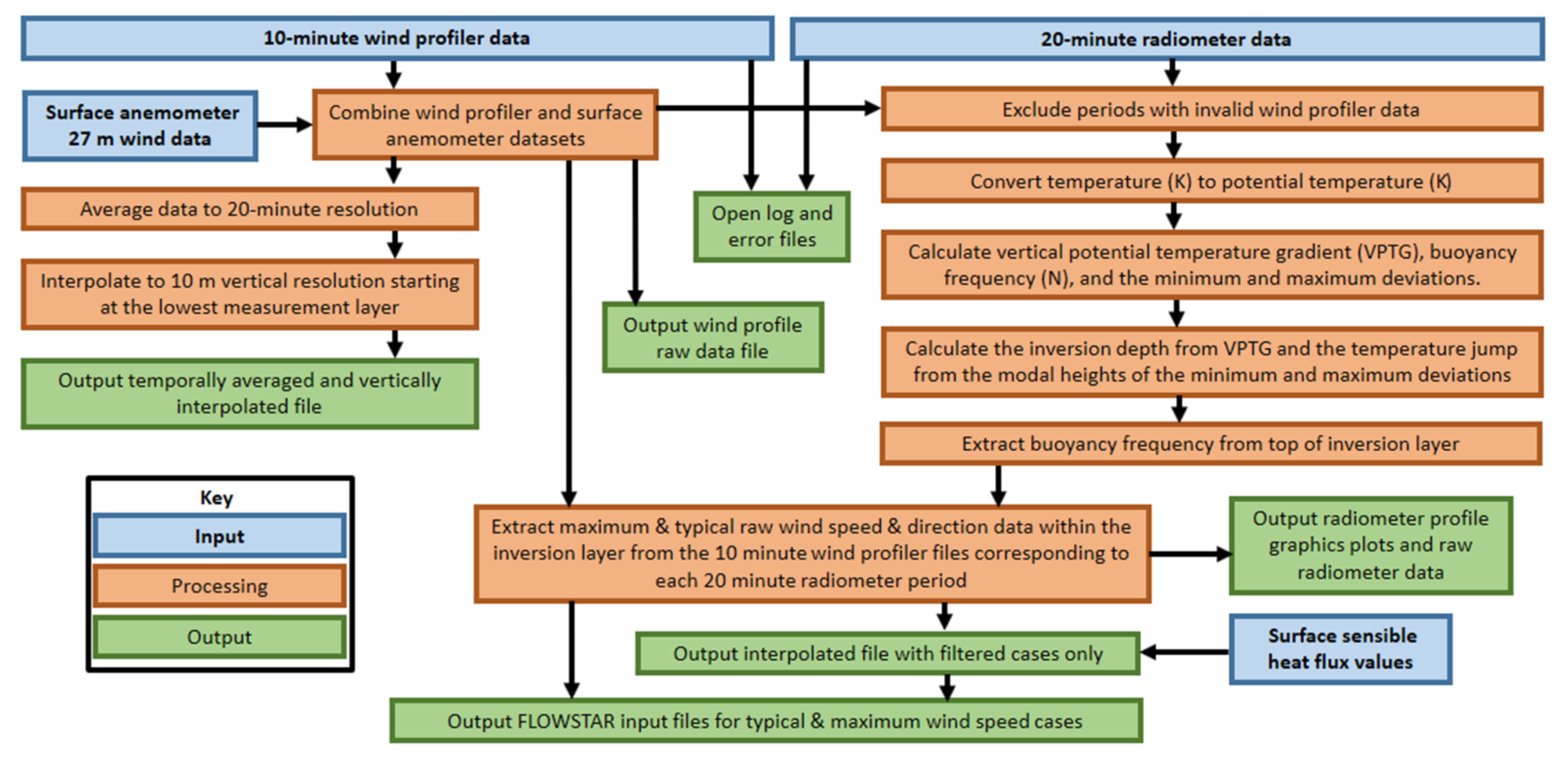
Figure 2 presents a flow chart that outlines key inputs, outputs and processing steps associated with the wind and temperature data processing. Processing details of the surface sensible heat flux calculations have been omitted from this flow chart because the marine boundary layer scheme calculations have been performed within an alternative model application, ADMS 5 [21] i.e., bespoke processing scripts were not required. ADMS 5 is an atmospheric dispersion modelling tool developed by Cambridge Environmental Research Consultants (UK), used extensively by commercial, research and regulatory organizations worldwide for the calculation of air quality impacts resulting from the release of atmospheric pollutant emissions from industrial installations. The model includes a meteorological pre-processing module that derives meteorological parameters used to describe the atmospheric boundary layer, such as surface sensible heat flux, from meteorological measurement datasets; this module has been used for the marine boundary layer calculations described here.

The methods described in the following sections describe the meteorological processing steps for valid data points; error handling to allow for invalid and missing data has been included in the processing, but full details have been omitted for brevity.

2.2.1. Radiometer Data Processing

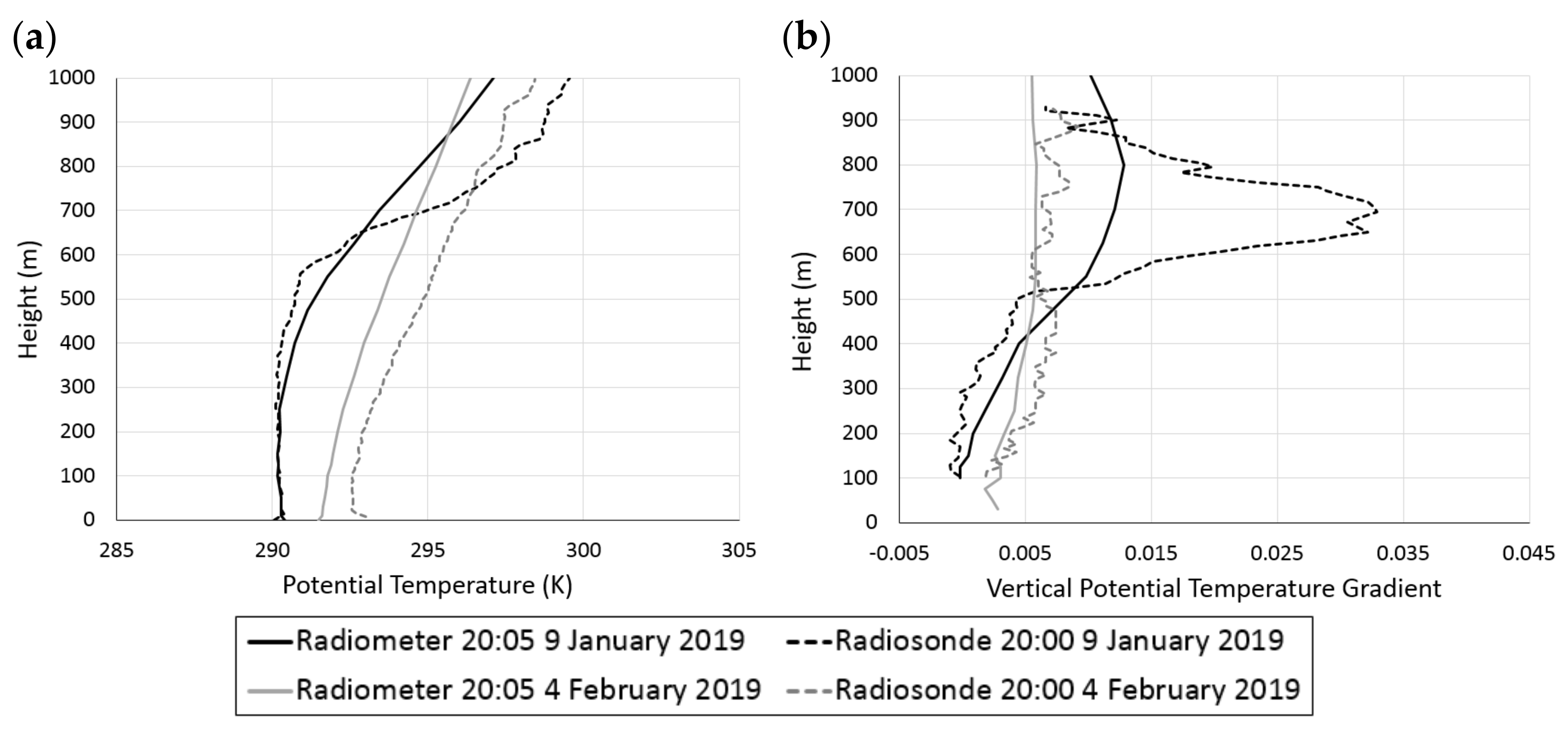
Inspection of radiometer data indicates that values compare well with the more reliable radiosonde temperature records in terms of overall values, but the gradient does not appear to detect elevated temperature inversions; this has been reported previously in the literature [22]. Figure 3a presents an example demonstrating this (20:00 9 January 2019), where the radiosonde clearly indicates a temperature inversion between approximately 550 and 850 m; the radiometer does not detect the changes in gradient with height shown by the radiosonde. Figure 3a also presents the same comparison for a different time (20:00 4 February 2019), when no clear inversion is detected by the radiosonde; the profiles compare well for the first few hundred metres, but accuracy decreases with height. However, despite the radiometer’s inability to precisely capture the potential temperature variations with height, the similarities between the profiles provide motivation for development of methods that extract the required information from the high temporal resolution radiometer data.

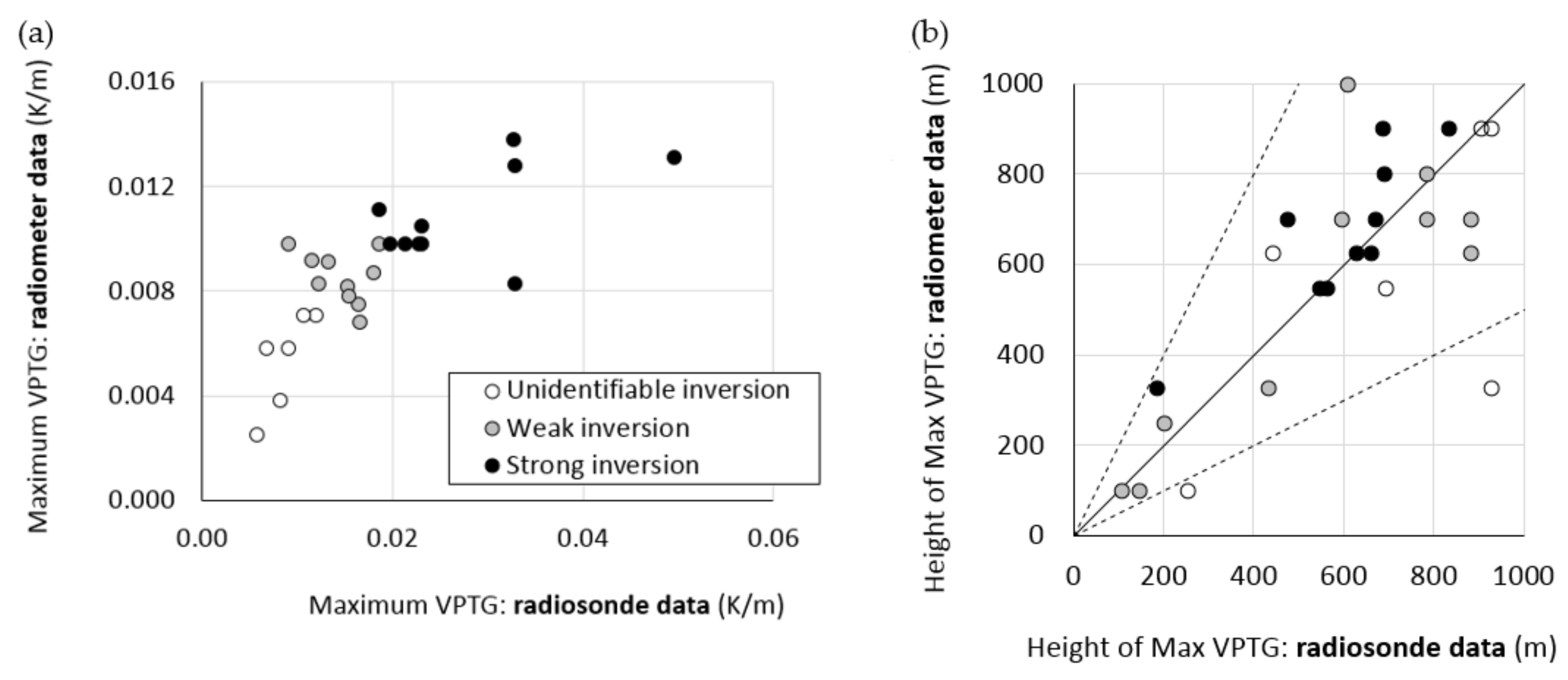
Estimates of boundary layer height, potential temperature jump in the inversion layer and the buoyancy frequency at the top of the inversion layer must be derived from the radiometer data (Table 1). The most straightforward way to derive an estimate of the boundary layer height for atmospheric conditions in which a temperature inversion is present is to calculate the maximum gradient with respect to height above ground of the potential temperature profile. Figure 3b compares example radiosonde and radiometer vertical potential temperature gradient (VPTG) profiles, where the VPTG is calculated using potential temperature values from immediately below and above the specified height. The strong inversion case (9 January) shows that whilst the magnitude of VPTG for the radiosonde is much greater than that for the radiometer, both temperature gradient profiles have clear maximum values in near-identical locations. Conversely, neither radiosonde nor radiometer VPTG values for the 4 February indicate a clear maximum value. Of note here is that there is much less ‘noise’ associated with the radiometer VPTG profiles compared to the corresponding radiosonde profiles, which simplifies the identification of the location of the maximum value, although there are some sharp changes in near-ground profiles.

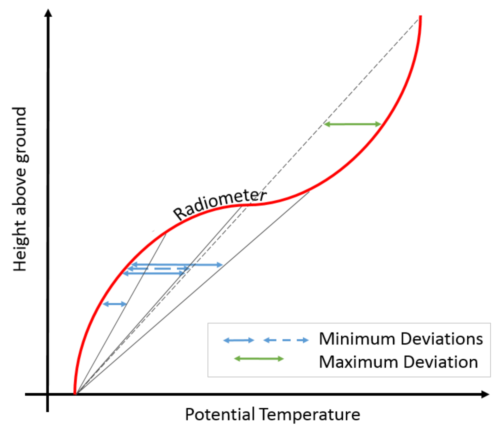
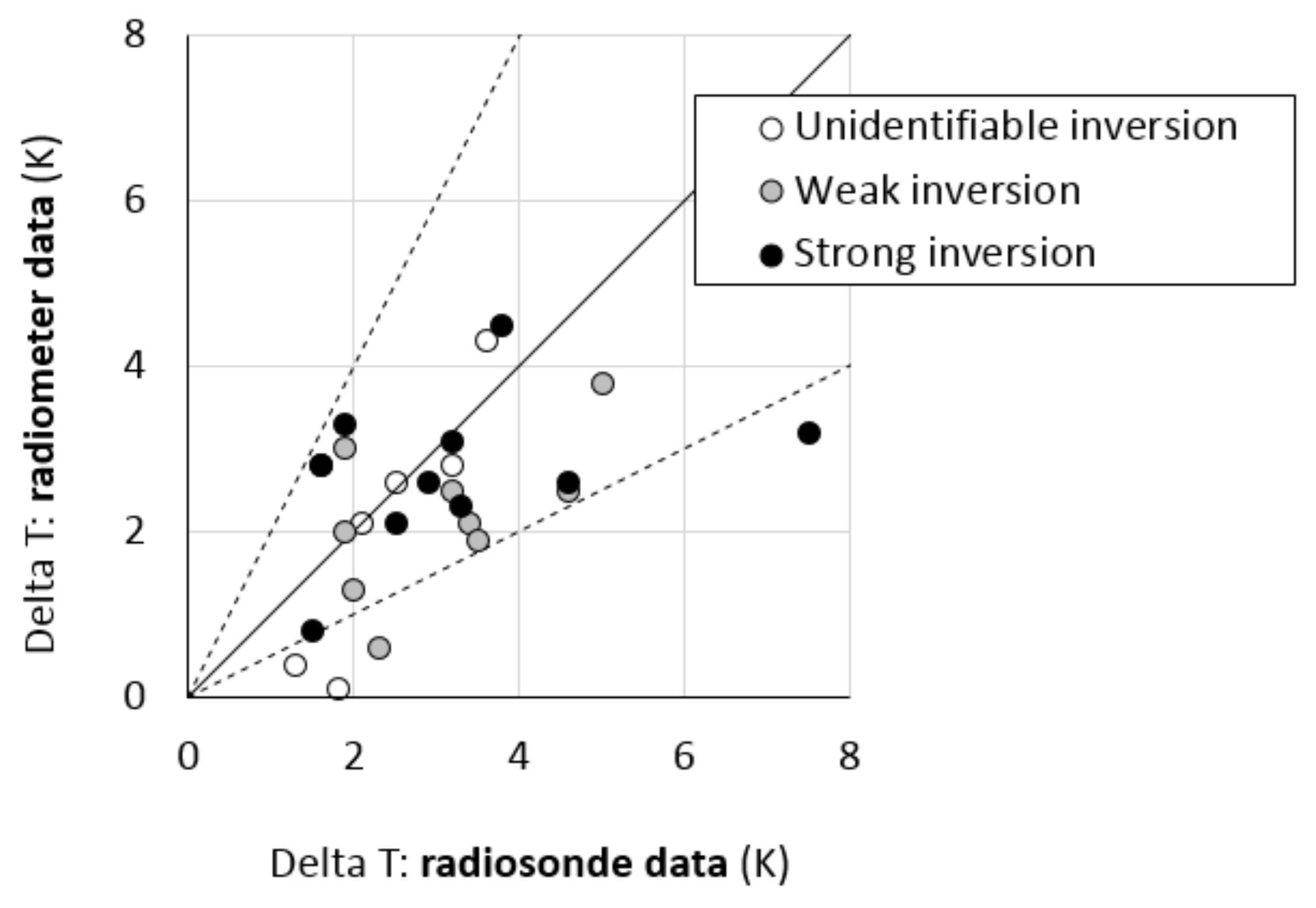
Following the identification of the temperature inversion height from the radiometer profile data, a novel approach has been developed to estimate the corresponding inversion strength, by amplification of the profile variation. Inspection of Figure 3a and multiple other potential temperature profiles leads to the conjecture that a profile with a strong inversion has a distinctly non-linear profile; conversely, where no inversion is present, the potential temperature increase is close to linear. Thus, if minimum and maximum deviations from linear increases in potential temperature profiles are calculated, then the magnitude of the temperature jump may be estimated. Figure 4 presents the variation of an idealized radiometer potential temperature profile with height. The concept of the calculation of deviations from a linear profile (i.e., straight line) starting at the ground and increasing with height at equally spaced intervals is shown. For each linear profile, a series of values corresponding to the temperature difference between the straight line and the radiometer profile are calculated, corresponding to each linear profile height value; these differences can be negative or positive. Then, for each linear profile, the ‘minimum deviation’ is set equal to the largest magnitude negative difference between the profiles (indicated by the blue arrows in Figure 4) and the ‘maximum deviation’ is set to the largest magnitude positive difference between the profiles (the green arrow on Figure 4). A series of minimum and maximum deviations are calculated (i.e., one for each height above the ground), and the corresponding height of the minimum/maximum deviation is recorded together with the associated potential temperature value. As can be seen by the schematic (Figure 4), heights corresponding to relatively sharp gradient changes are recorded repeatedly; this method allows the application of a ‘modal’ approach to identification of the location of the minimum/maximum deviation from a linear profile; the temperature jump is estimated by the difference between the potential temperature recorded at the height of the maximum deviation and the potential temperature at the height of the minimum deviation. When applying this calculation methodology to measured meteorological parameters, it is important to perform error checking, for instance, to ensure that the calculated height of the minimum deviation is below the height of the temperature inversion, which is also below the height of the maximum deviation.

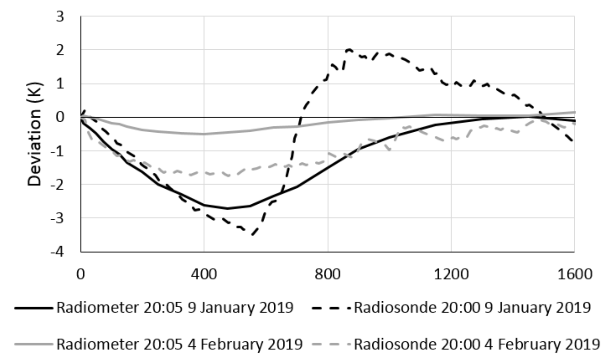
Example results of these deviation calculations are shown in Figure 5 as a comparison between radiometer and radiosonde deviations; the deviation calculations correspond to a linear profile extending to 1.5 km. For the strong temperature inversion example shown (9 January), the radiosonde profile deviates significantly from the linear profile; the corresponding radiometer calculation shows a similar trend for the minimum deviation, although no maximum deviation is identified. The weak inversion case (4 February) demonstrates much smaller deviations for both the radiosonde and the radiometer.

The remaining parameter required as input to the FLOWSTAR model is an estimate of the buoyancy frequency above the boundary layer. Buoyancy frequency is directly related to the derivative of the potential temperature gradient with respect to height. As can be seen from Figure 3b, the radiometer potential temperature gradient varies slowly above the inversion layer, making precise identification of the ‘top’ of the boundary layer difficult. A practical solution to the calculation of this parameter is therefore to associate the height of the maximum deviation with the top of the inversion layer and to use the associated buoyancy frequency.

2.2.2. Wind Profiler and Surface Anemometer Data Processing

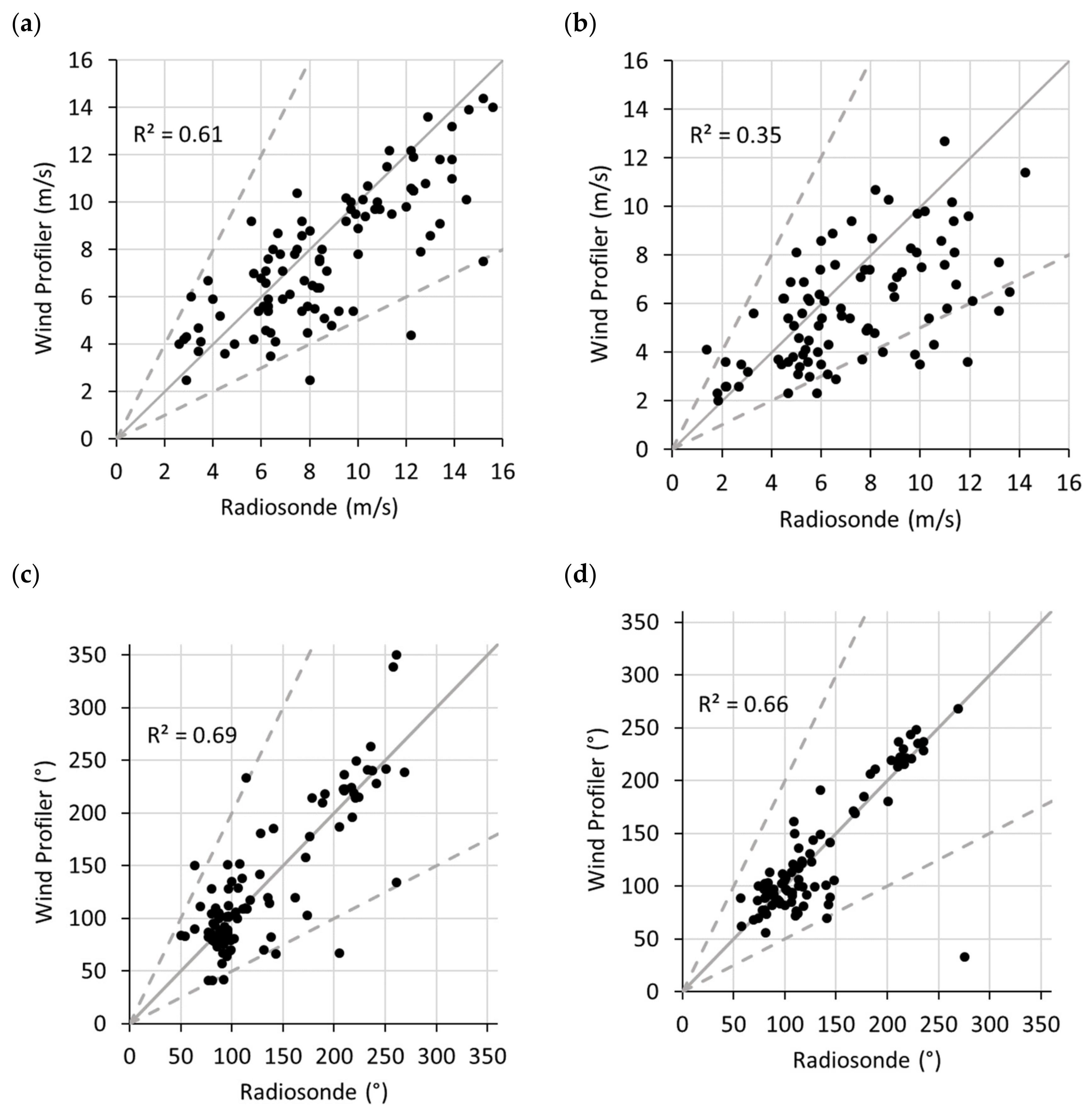
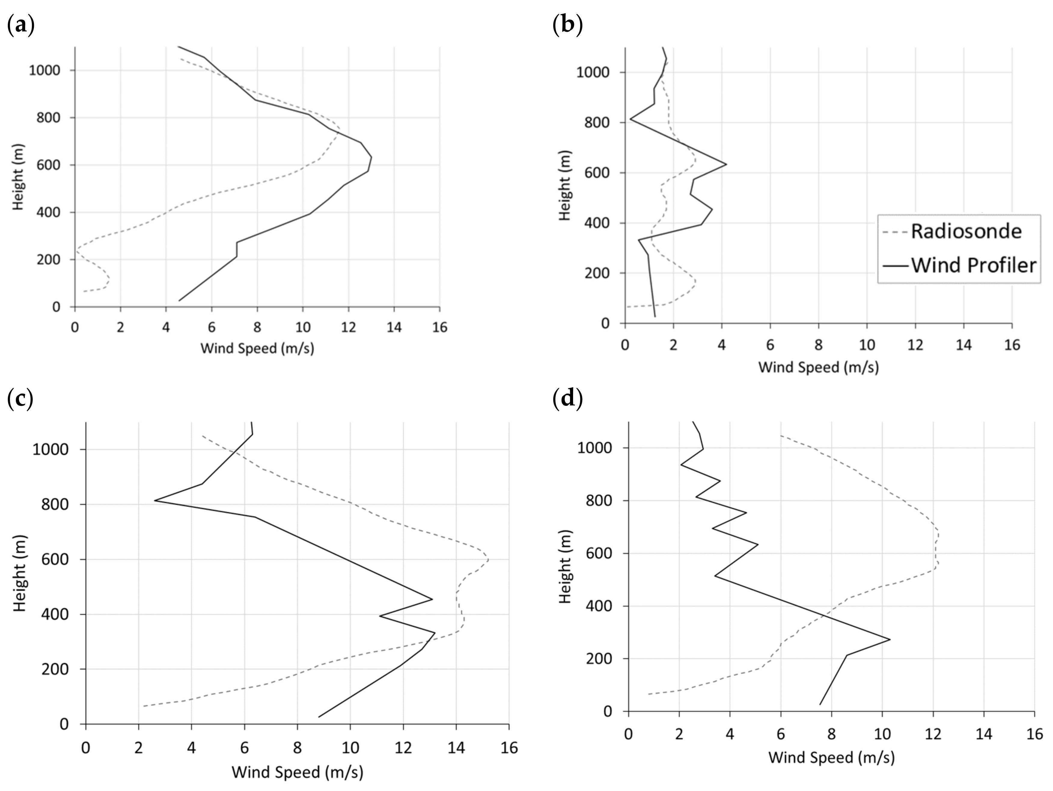
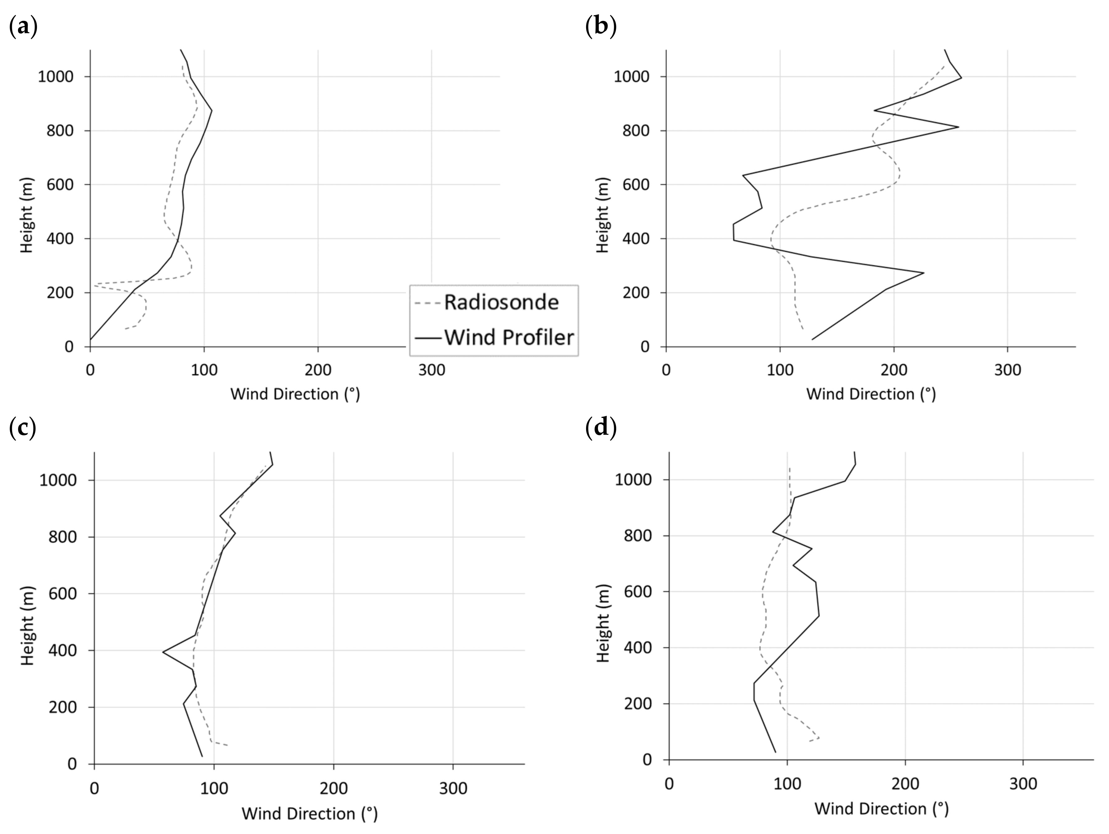
The instruments located at Cheung Chau (CCH), a small island upwind of Lantau Island, include a surface anemometer and a wind profiler; temporal resolutions of these measurements differ from the radiometer (Table 2) so temporal interpolation must be applied to hourly wind anemometer data to approximate wind values at 20-min resolution, with temporal averaging applied to derive 20-min vertical wind profiles from the 10-min data recorded by the profiler. The lack of wind data between approximately 27 m and 200 m above the surface is a limitation of the current methodology to describe in detail the near-surface flow structure, although the lack of resolution may not be crucial for the FLOWSTAR modelling approach, where the wind speed in the inversion layer governs the strength of the mountain waves influencing air flow at the airport. Due to the influence that the magnitude of the inversion layer wind has on model predictions, previous work [17,18] has considered both maximum and typical inversion layer wind speeds and directions. Consequently, two sets of parameters are calculated for the current study. The sparsity of wind profiler measurements also influences the accuracy of the wind flow calculations.

In addition to the temporal averaging described above, linear interpolation is used to estimate the wind profile in the height range from 27 m to approximately 200 m; this approach could be refined by applying a more representative logarithmic profile, which would require surface roughness estimates, for instance, as calculated during the marine boundary layer calculations described below.

Mountain waves are generated by the flow of air masses over Lantau Island to the southeast of HKIA for particular meteorological conditions; winds from other directions under similar atmospheric stability conditions are unlikely to generate sufficiently severe mountain waves to cause disruption. Therefore, the meteorological data were filtered to exclude cases when the wind direction in the inversion layer does not indicate flow over Lantau Island.

2.2.3. Weather Buoy Data Processing

Data from weather buoys WB1 and WB4 have been used to estimate a surface sensible heat flux suitable for representing atmospheric conditions in a near-marine environment. Sea surface temperature is recorded every minute, whereas the associated 8.5 m air temperature and wind data are available at hourly resolution. The sea surface data have therefore been averaged over each hour for use in processing alongside the remaining weather buoy measurements.

The weather buoy data processing methodology follows the marine boundary layer scheme implemented in the ADMS 5 atmospheric dispersion model. The method uses an estimate of the near-surface temperature gradient derived from the difference between sea surface and air temperature measurements and includes a wind speed-dependent sea surface roughness calculation. For surface roughness, the formula used by the European Centre for Medium range Weather Forecasts (ECMWF) is adopted:

$$z_0={\alpha }_m\frac{\mathsf{\nu }}{u_{*}}+{\alpha }_{Ch}\frac{u_{*}{}^2}{g}$$

(1)

ref. [23] where $u_{*}$ (m/s) is the friction velocity, ν (m²/s) is the kinematic viscosity of air, g (m/s²) is the acceleration due to gravity, α_m = 0.11, and α_Ch is the Charnock parameter, which has been set to 0.08 for this study.

The velocity profiles used are

$$\begin{array}{cc}U\left(z\right)=\frac{u_{*}}{\kappa }\left\{\ln \left(\frac{z+z_0}{z_0}\right)-\Psi \left(\frac{z+z_0}{L_{MO}},\frac{z_0}{L_{MO}}\right)\right\}& \hfill \mathrm{for}z\le h\\ U\left(z\right)=\frac{u_{*}}{\kappa }\left\{\ln \left(\frac{h+z_0}{z_0}\right)-\Psi \left(\frac{h+z_0}{L_{MO}},\frac{z_0}{L_{MO}}\right)\right\}& \hfill \mathrm{for}z>h\end{array}$$

(2)

where $\kappa$ is von Karman’s constant (0.4),$h$(m) is the boundary layer height and the Monin-Obukhov length $L_{MO}$(m) is given by

$$L_{MO}=-u_{*}^3\left(\frac{\rho c_p{T}_0}{\kappa g{F}_{{\theta }_0}}\right)$$

(3)

where c_p is the specific heat capacity of air (J/kg/K), ρ is the density of air (kg/m³),$F_{{\theta }_0}$ is the surface sensible heat flux (W/m²) and $T_0$ is the air temperature at the surface (K), and where under convective conditions ($h/L_{MO}<0)$ [24],

$$\begin{gathered} \Psi =\ln \left(\frac{{\left(1+x\right)}^2}{{\left(1+x_0\right)}^2}\frac{\left(1+x^2\right)}{\left(1+x_0^2\right)}\right)-2\left({\tan }^{-1}\left(x\right)-{\tan }^{-1}\left(x_0\right)\right) \\ x={\left(1-\frac{16\left(z+z_0\right)}{L_{MO}}\right)}^{1/4} \\ {x}_0={\left(1-\frac{16z_0}{L_{MO}}\right)}^{1/4} \end{gathered}$$

(4)

and in stable-neutral conditions ($h/L_{MO}\ge 0)$ [25],

$$\begin{gathered} \Psi =a\frac{z_0}{L_{MO}}+b\left(\frac{z_0}{L_{MO}}-\frac{c}{d}\right)e^{-d{z}_{\frac{0}{L_{MO}}}} \\ -\left\{a\frac{\left(z+z_0\right)}{L_{MO}}+b\left(\frac{\left(z+z_0\right)}{L_{MO}}-\frac{c}{d}\right)e^{-d\left(z+z_0\right)/L_{MO}}\right\} \end{gathered}$$

(5)

where the constants $a$ = 0.7, $b$ = 0.75, $c$ = 5.0 and $d$ = 0.35. The equations are solved by iteration.

Over sea, the surface roughness for sensible heat (z_0H) and moisture (z_0q) are given by [23]

$$z_{0H}={\alpha }_H\frac{\nu }{u_{*}}\mathrm{and}{z}_{0q}={\alpha }_q\frac{\nu }{u_{*}}$$

(6)

where α_H = 0.4 and α_q = 0.62. The sensible heat flux $F_{{\theta }_0}$ is then given by

$$F_{{\theta }_0}=\frac{-c_p\rho {\kappa }^2\left(\theta \left(z\right)-{\theta }_0\right)u\left(z\right)}{\left[\ln \left(\frac{z+z_{0H}}{z_{0H}}\right)-{\Psi }_H\left(\frac{z+z_{0H}}{L_{MO}}\right)\right]\left[\ln \left(\frac{z+z_0}{z_0}\right)-\Psi \left(\frac{z+z_0}{L_{MO}}\right)\right]}$$

(7)

where θ is potential temperature (K), and θ₀ is the potential temperature corresponding to the temperature of the sea surface [24].

For stable and neutral conditions, ψ_H = ψ, and for convective conditions, ψ_H is given by

$${\Psi }_H=\ln \left(\frac{{\left(1+y\right)}^2}{{\left(1+y_{surface}\right)}^2}\right)$$

(8)

where

$$y={\left(1-\frac{16\left(z+z_{0H}\right)}{L_{MO}}\right)}^{1/2}\mathrm{and}{y}_{surface}={\left(1-\frac{16z_{0H}}{L_{MO}}\right)}^{1/2}$$

(9)

The latent heat flux λE is given similarly by

$$\lambda E=\frac{-\lambda \rho {\kappa }^2\left(q\left(z\right)-q_{sat0}\right)u\left(z\right)}{\left[\ln \left(\frac{z+z_{0q}}{z_{0q}}\right)-{\Psi }_q\left(\frac{z+z_{0q}}{L_{MO}}\right)\right]\left[\ln \left(\frac{z+z_0}{z_0}\right)-\Psi \left(\frac{z+z_0}{L_{MO}}\right)\right]}$$

(10)

where λ is the specific latent heat of vaporization of water (J/kg), q is the specific humidity, q_sat0 is the saturation specific humidity at the sea surface and ψ_q = ψ_H. Again, the equations are solved by iteration [24].

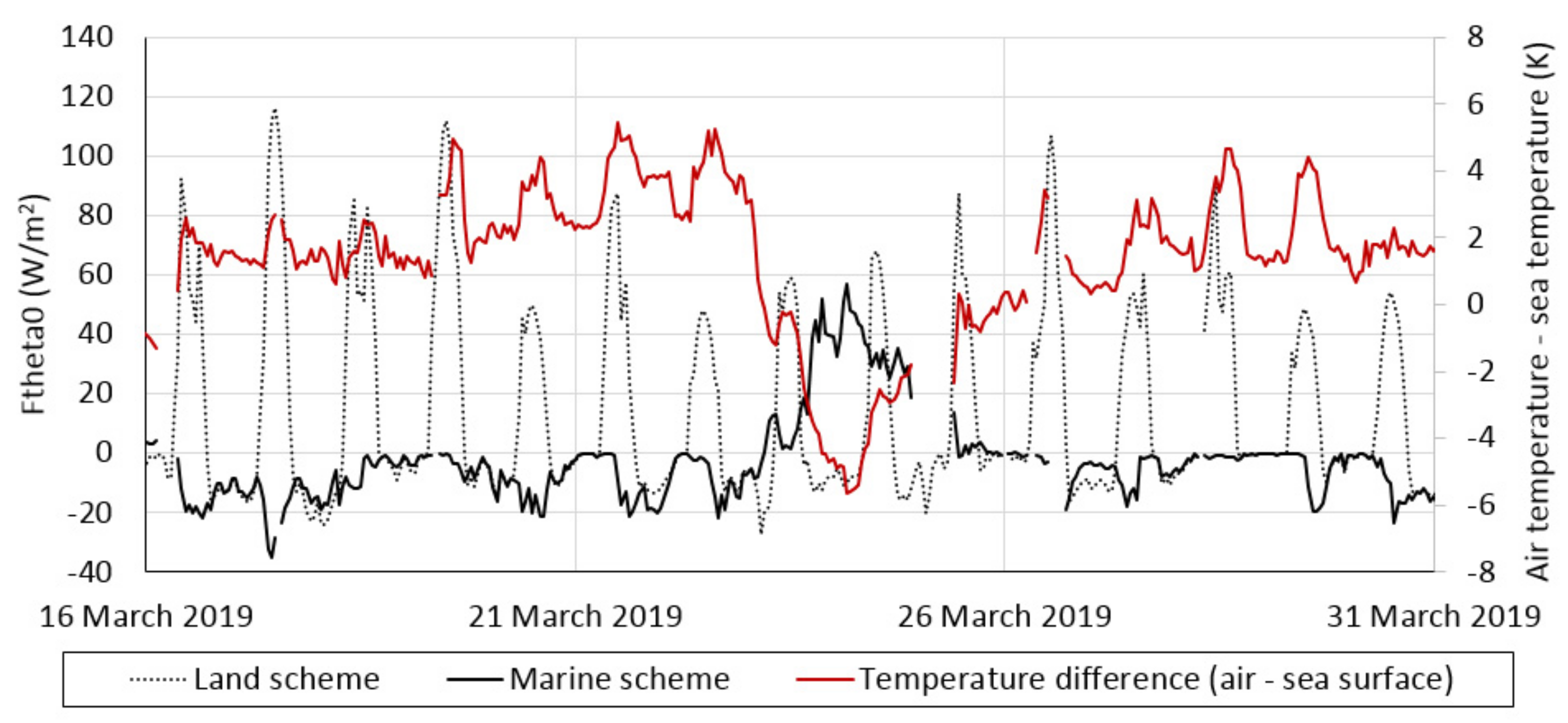
Marine heat flux parameter measurements are unavailable for direct comparison against calculated values. Instead, the evaluation method applied is to compare the calculated marine heat flux values to the corresponding estimates of the heat flux values from a land surface scheme [25], which uses cloud cover and surface air temperatures as input.

3. Results

The results presented in this section relate to the period January to April 2019. For temperature-related parameters, an inter-comparison of datasets derived from the radiometer and radiosonde has been undertaken for the subset of hours where radiosonde soundings are available (27 h); wind profiler measurements can similarly be compared to radiosonde soundings, and a comparison of hourly marine and land surface sensible heat flux values is presented.

3.1. Radiometer Data Processing Evaluation

The radiometer data processing outputs are estimates of the boundary layer height, temperature jump in the inversion layer and buoyancy frequency at the top of the boundary layer; in addition, the magnitude of the associated VPTG parameter provides an indication of the strength of the temperature inversion. Within the set of radiometer measurements made at times that coincide with radiosonde soundings, the purpose of this work is to identify a further subset of cases that corresponds to stronger inversions, which can be defined in terms of sharp changes in potential temperature profiles (i.e., high maximum VPTG) and large associated temperature jumps. It is clear from inspection of a series of radiometer and radiosonde profiles similar to Figure 2 (as part of this and earlier work) that any VPTG threshold criteria used to identify strong inversions will differ for the radiosonde and radiometer because the radiosonde identifies a much sharper temperature gradient compared to the radiosonde. For this study, only data points within the lowest 1000 m have been considered because strong, low inversions are the most likely to generate mountain waves.

The method applied to evaluate the derived maximum VPTG values is to compare the values directly (Figure 6a); this figure indicates that the radiometer values broadly correlate with the radiosonde values, but the radiosonde maxima are much higher, as expected. Critical to this evaluation is the identification of the strongest inversions, so subsets of cases have been defined in the following way:

• Strong inversions: all cases above the 66th percentile of maximum VPTG values for the radiosonde or radiometer (10 cases);
• Weak inversions: all cases above the 33rd percentile of maximum VPTG values for the radiosonde or radiometer, if not included in the strong inversions subset (10 cases); and
• Unidentifiable inversions: all other cases (six cases).

Figure 6a indicates that, in general, the radiometer strong inversion maximum VPTG values correlate with the corresponding values derived from the radiosonde, with one outlier. Maximum VPTG values for the weak inversions are grouped for the two approaches, although there is no clear correlation within this subset of values.

The next step is to compare the heights at which the maximum VPTG values have been identified, that is, the inversion heights. The boundary layer height can be set equal to, or derived from, this inversion height, for instance, by taking into account the inversion layer depth in some way. Figure 6b compares the heights of the maximum VPTG measured by the two instruments; the heights range from 100 m to the maximum depth considered (1000 m). There is good agreement between the heights derived using the two instruments, with 100% of the radiometer heights being within a factor of two of the radiosonde heights for the strong and weak inversions subsets. The heights associated with the strong inversion are in better agreement than those corresponding to the weak inversions. Whilst weak inversions are identified at all heights, the stronger inversions in general relate to 500–1000 m.

The final parameter derived from the vertical potential temperature profiles is the temperature jump; a comparison is shown in Figure 7. There is broad agreement between the two datasets, although the radiometer has a tendency to under-predict some of the higher temperature jumps derived from the radiosonde profiles; 90% of cases are within a factor of two for the strong inversion subset, with the remaining cases under-predicting the temperature jump. Agreement is similar for the moderate subset; again, 90% of cases are within a factor of two.

The aim of this work is to prescribe inversion layer parameter threshold criteria that will lead to the automatic identification of strong inversions; the maximum VPTG and temperature jump are the most suitable parameters for this purpose. This evaluation indicates that no clear threshold criteria can be specified that would lead to a direct correspondence between radiosonde and radiometer profiles because, for instance, there is no exact cut off distinguishing the strong from weak inversion cases in terms of maximum VPTG (Figure 6). However,

Table 3. Summary of criteria that could be used to classify strong and moderate inversions for radiometer and radiosonde datasets.

Inversion Classification	Maximum Vertical Potential Temperature Gradient (K/m)		Temperature Jump (K)
	Radiometer	Radiosonde	Radiometer	Radiosonde
Strong	0.009	0.002	2	2
Moderate	0.008	0.015

summarizes the threshold criteria that, if applied for the subset of cases evaluated here, would lead to identification of at least some of the cases; it is the temperature jump values that appear to correlate least well, and refinements of the derivation of this parameter from the points identified as the minimum and maximum deviations may be possible.

3.2. Land Wind Data Processing Evaluation

The radiosonde soundings were recorded approximately 19 km from the CCH measurements, so a difference in the measurement profiles is to be expected, particularly near the ground. Two sets of wind speed and direction parameters are compared: values corresponding to the typical (average) and values corresponding to the maximum wind speed in the inversion layer. Figure 8 presents scatter plots comparing wind speed and direction parameters. In general, the wind speed values recorded by the wind profiler are similar or slightly lower than the radiometer wind speeds (Figure 8a,b). Correlation between measured values is better for the maximum wind speed than for the typical values; the likely explanation for this is that typical (average) values are dependent on the vertical extent of the inversion layer, and this dimension is difficult to define precisely using the radiometer data due to the shallow vertical temperature gradients.

Wind directions compare better than the wind speeds, with good correlation and agreement corresponding to both the maximum and typical wind speed cases. The prevailing wind direction for the period considered can be identified from the wind direction scatter plots, that is, in the range 50 to 150 degrees; it is of note for the current study that these wind directions correspond to air advecting over Lantau island toward the airport. There is also a subset of wind directions corresponding to southwesterly winds.

The relative accuracy of wind profiles has been compared for a selected number of time periods. Figure A1 and Figure A2 in Appendix A show the wind speed and wind direction profiles respectively, for four time periods. Considering the distance between the measurement sites, both the wind speed and direction compare well for most cases, although the ground level wind speed is generally lower at King’s Park than on Cheung Chau island; this may be explained by the relatively remote and exposed CCH location. The one example of a low wind speed case (25th March) corresponds to a variable wind direction profile, for which both instruments are in broad agreement; of the remaining high wind speed cases, 15th April shows poor agreement for wind speed, but the wind directions compare well.

3.3. Marine Surface Sensble Heat Flux Data Processing Evaluation

Ideally, the weather buoy measurements used as input to the surface sensible heat flux calculations would be taken from the same buoy for the full period. Unfortunately, weather buoy data capture was relatively sparse for the period January to April 2019, necessitating the requirement to merge data from WB1 to the west of the airport with WB4 to the east (Figure 1); an averaging approach was taken for both temperature and wind speed measurements where data from both buoys were available. The combined dataset resulted in marine calculations for 70% of the time period and land calculations for 84% of the period.

Figure 9 presents a time series of marine and land surface sensible heat flux values for the period 16 to 31 March 2019; the difference between the land and sea surface temperatures is also presented. There was comprehensive data capture for both buoys for this period and good inter-buoy agreement of the relevant parameters. As expected in spring, the air temperature is typically warmer than the sea since the sea only warms slowly after the winter; this results in a stable marine boundary layer. Thus, in general, surface sensible heat flux values over the sea and land are similar at night since the land boundary layer is also stable with minimum heat fluxes of around –20 W/m². Conversely, during the day, the marine and land values diverge, since the land fluxes demonstrate a diurnal variation that correlates with solar intensity, with peak values around midday in the range 50 to 120 W/m². The daytime marine heat flux values remain predominantly stable, with a minimum value of close to –40 W/m²; the exception to this is the period 23–24 March where the day and night time marine values correspond to convective conditions, reaching a maximum of nearly 60 W/m². This episode of high marine surface sensible heat flux values correlates with a period when the sea surface temperature is greater than the air temperature, shown by the red line on Figure 9. HKO records state that a cold front moved across the coast of Guangdong during this period, bringing colder air to the region.

In order to better understand the meteorological conditions associated with the episodes when the marine surface sensible heat flux exceeds the land flux value, Figure 10 shows the variation of the difference between the parameters (land minus marine) with the wind speed and direction in the form of a polar plot; data for the four-month period are shown. This plot shows that stable flows are associated with milder winds from south west to east and convective flows with colder winds from the north and north-east.

4. Discussion

The motivation for this paper has been to identify measurement instrumentation that operates in real time and at high temporal resolution that is able to generate meteorological parameters suitable for input into the FLOWSTAR flow field model. The instrumentation identified for this purpose are: a microwave radiometer at King’s Park; a wind profiler and surface anemometer on Cheung Chau Island; and weather buoys located in the Pearl River estuary, deployed in close proximity to the airport. All datasets require processing in order to derive the subset of parameters required by the model, specifically: boundary layer height, wind speed and direction in the inversion layer, wind direction vertical profile in the boundary layer, surface sensible heat flux, potential temperature jump in the inversion layer and buoyancy frequency at the top of the inversion layer.

The novel approach to the identification of inversion layer quantities from radiometer profiles has been described and then evaluated using radiosonde measurements. The approach works well in terms of the identification of the height of the temperature inversion, although associated temperature jump estimates are less accurate. Wind data in the inversion layer derived from wind profiler data compare generally well with radiosonde measurements, with agreement for parameters corresponding to the maximum wind speed being more accurate than those related to ‘typical’ wind. Surface sensible heat flux measurements are unavailable in the vicinity of HKIA, so an inter-comparison of modelled marine and land fluxes has been presented. For the springtime period studied, the marine fluxes are comparable to the land values at night, but marine fluxes remain stable during the day whilst land fluxes follow a convective cycle that correlates with solar intensity. For particular meteorological conditions where cold winds advect from the north/north east of HKIA, the marine boundary layer becomes unstable for prolonged periods.

With the exception of the surface sensible heat calculation, the methodologies developed for this work have been automated in a series of R scripts [27]. These scripts facilitate the automatic processing of large datasets. For the work presented here, data for the period January to April 2019 have been processed, at 20-min resolution, generating more than eleven thousand meteorological inputs representing both ‘typical’ and ‘maximum’ wind speed conditions. The scripts are suitable for inclusion within a wind shear now-casting system.

There are many uncertainties associated with the accuracy of the meteorological parameters generated. Some uncertainties arise from the spatial separation of the measurements used as input to the system (Chek Lap Kok, King’s Park and Cheung Chau island), which may lead to inconsistencies between the datasets. An approach that allows for the time taken for an air mass to travel from Cheung Chau island to the airport may partially address this issue. The limitations of the radiometer dataset in terms of the lack of resolution of sharp temperature gradients contributes to uncertainty, and the wind profiler measurements can be sparse. It may be possible to deploy additional measurement equipment that samples at finer vertical resolution and is better able to characterize the atmospheric boundary layer, for instance, dropsondes released from aircraft [28]. The deployment of drone aircraft releasing dropsondes could form part of a nowcasting system, although it may be difficult to incorporate such equipment within an operational system due to the requirement of high temporal resolution datasets. If this methodology is included in an operational now-casting application, the generation of a data quality flag for each time period is recommended.

This study has focused on generation of meteorological data inputs for a FLOWSTAR model application able to identify mountain waves. However, other meteorological conditions give rise to wind shear at the airport, which are not identified by the current methodology, for instance, strong wind veering and backing upwind of the airport. This is a limitation of the current approach that would have to be addressed in an operational now-casting system because further work would be required to incorporate the automatic identification of other adverse meteorological conditions within the system.