Abstract
Identifying changes in ambient air pollution levels and establishing causation is a research area of strategic importance to assess the effectiveness of air quality interventions. A major challenge in pursuing these objectives is represented by the confounding effects of the meteorological conditions which easily mask or emphasize changes in pollutants concentrations. In this study, a methodological procedure to analyze changes in pollutants concentrations levels after accounting for changes in meteorology over time was developed. The procedure integrated several statistical tools, such as the change points detection and trend analysis that are applied to the pollutants concentrations meteorologically normalized using a machine learning model. Data of air pollutants and meteorological parameters, collected over the period 2013–2019 in a rural area affected by anthropic emissive sources, were used to test the procedure. The joint analysis of the obtained results with the available metadata allowed providing plausible explanations of the observed air pollutants behavior. Consequently, the procedure appears promising in elucidating those changes in the air pollutant levels not easily identifiable in the original data, supplying valuable information to identify an atmospheric response after an intervention or an unplanned event.
1. Introduction
Air pollution is one of the biggest environmental threats to human health, alongside climate change [1]. To safeguard people’s health, the design of effective and well-targeted strategies aimed at preventing or reducing health damages associated with the exposure to the atmospheric pollution [2], as well as the assessment of the effectiveness of air quality interventions [3], are required. Both these issues can profit by the development of tools that allow understanding the changes and behaviors of air pollutants over time and establishing whether a change can be attributed to a known cause [4]. However, assessing the variability of ambient air pollution or establishing causation can be highly challenging due, for example, to the known effects of meteorological conditions that strongly affect air pollutants levels over multiple scales in time and space [5,6,7]. The process of accounting for changes in meteorology over time in an air quality time series, which is referred to as the “meteorological normalization” process, can be carried out through several statistical techniques [8,9], ranging from models based on linear regression [10] to neural networks [11]. A new approach based on machine learning (ML) random forest (RF) predictive algorithms, having better performances than traditional statistical methods [12], has recently emerged [13,14,15] and open-source implementation of these algorithms in the R language is also available [16]. Once the confounding weather effects have been removed, more robust statistical evaluations can be carried out to understand the changes and behaviors in the resulting normalized time series because there is more certainty that the observed trends are due to changes in emissions rather than changes in meteorology. This is the case, for example, of the detection of change points (i.e., unexpected structural changes in time series data properties, such as the mean or variance [17]), and of the trend patterns analysis, (i.e., concentration changes over a period of time [18]). The change points detection and trend investigation in time series are of interest in many sectors ranging from genetic to finance [19]. In the environmental field they have a widespread applicability due to their significant implications for pollution control and for environmental decision-making [20,21,22,23]. In the context of the air pollution studies, change points can be representative of station relocation, changes of instrumentation and/or changes concerning the sources around the measurement station. The trend analysis instead examines if statistically significant changes occur in pollutant concentrations over time.
The aim of the work is to develop a methodological procedure to assess and explain the changes in pollutant concentrations levels once the confounding effects of weather have been accounted for. To this end, we developed a three-stage methodology. First, the effects of local weather in the air quality time series were disentangled using a technique of meteorological-normalization based on an RF-ML algorithm. Secondly, the tandem use of both the change points detection and trend analysis was adopted to investigate the normalized signal. Finally, a joint examination of the results obtained by the first two stages and the available metadata on the air pollution sources was carried out. The developed methodology was applied on a dataset comprising daily averaged data of air pollutants concentrations and meteorological parameters as well as temporal variables. Data were collected, over the 2013–2019 period, in a rural area of Southern Italy characterized by the proximity to populated areas of hydrocarbons extraction activities and pre-treatment. The current scientific evidence identifies the adverse impact of upstream oil extraction to air quality, although a low level of measured pollutant concentrations is also highlighted [24]. Knowledge gaps still exist regarding the impact on human health of the exposure to contaminants emitted by onshore hydrocarbon exploration and exploitation activities, especially regarding chronic exposures to low-levels of contaminants [25,26].
The procedure illustrated in the present work reveals promising in elucidating the changes in the air pollutant levels that are not easily identifiable in the original data and in identifying an atmospheric response after an intervention or an unplanned event [3]. Finally, it is expected that the proposed procedure can also be worthwhile applied to assess the atmospheric response to social and anthropic activities lockdown established in Italy in the first part of 2020 to fight the spreading of the coronavirus disease (COVID-19) [27,28].
2. Materials and Methods
2.1. Study Area
The area investigated in the present study is the Agri Valley, located in the South-West part of the Basilicata Region (Southern Italy), at approximately 600 m above sea level (Figure 1). The valley extends for approximately 1400 km2 in a NW-SE direction, bordered, on both sides, by the Apennines Mountains and is partially included in a National Park (Parco Nazionale dell’Appennino Lucano-Val d’Agri-Lagonegrese); it hosts a population of approximately 50,000 inhabitants distributed in several small hilltop towns surrounding the valley. The strong peculiarity and criticality of this area is determined starting from the 2000s, when the predominantly rural typology of the area, characterized by the presence of woods, agricultural and breeding zones, has been altered by the start of hydrocarbons extraction activities near inhabited centers. The valley, indeed, houses the largest on-shore western European reservoir of crude oil and gas and an oil pre-treatment plant (identified as Centro Olio Val d’Agri—hereafter COVA) in a populated area. More specifically, 24 oil wells are currently operating producing approximately 63% of the entire national oil production [29], making the COVA plant of strategic importance for the country. The plant produces conveyed and diffuse (included fugitive) emissions of gases and particulate, which can affect the air quality and potentially pose health risks for the population living in the area. Moreover, flaring and venting of petroleum-associated gas is another significant source of greenhouse gas emissions and airborne contaminants [30]. It is also worth mentioning that the industrial processes taking place in the plant involve dangerous substances for human health and the environment (toxics and flammables), exposing the plant to the risk of a major accident [31]. A moderate volume of light and heavy vehicular traffic along the main national road crossing the valley (SS598), together with domestic heating and farming activities, represent other contributors to the local atmospheric pollution. Finally, the geographical position in the center of the Mediterranean makes the area also subject to the transport of mineral dust from the Sahara desert [32].
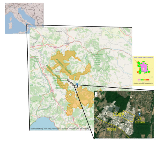
Figure 1.
Map of the study area and wind rose based on the hourly data at the VZI station over the study period (2013–2019).
The air quality control network operating in the area, managed by the Environmental Protection Agency of the Basilicata Region (ARPAB), consists of 5 monitoring stations. According to the requirements of the EU Air Quality Directive 2008/50/EC [33], ARPAB provides continuous concentration measurements of regulated pollutants (such as, among others, nitrogen oxides (NOX), sulfur dioxides (SO2), carbon monoxide (CO)), and of several pollutants specifically related to oil/gas extraction activities (such as hydrogen sulfide (H2S)). All monitoring stations are also equipped with instruments providing standard meteorological variables, such as temperature (T), atmospheric pressure (p), relative humidity (H), solar radiation (SR), wind direction (wd), and wind speed (ws). More details about the methods and the instrumentation used for the measurements can be found elsewhere [34], [35]. After the application of data quality procedures on the raw data, based on the data quality control process described in [36], ARPAB makes available to the public the hourly concentrations values of all measured parameters. For the purpose of this work data were obtained from the monitoring station closest to the COVA plant, named Viggiano (VZI, 40°18′50′′ N, 15°54′16′′ E, 603 m above sea level), categorized as an industrial station in a rural area. It is located at approximately 350 m from the industrial site and about 1 km from the national road SS598.
2.2. Observational Dataset
Four gaseous pollutants, which can be considered as proxies of the anthropic sources existing in the area, namely NOx, SO2, CO and H2S, were selected for the analysis. NOX, SO2 and CO represent the main component of the conveyed emission produced by the COVA plant [37]. For these pollutants, a strong evidence of respiratory and cardiovascular health effects is documented [38]. H2S is a toxic gas specifically related to oil/gas extraction activities carried out in the examined area and associated to diffuse (included fugitive) emissions [39]. Human exposure to the toxic effects of H2S is characteristically dose related and most notably involves the nervous, cardiovascular, and respiratory systems [40].
Hourly data of NOX, SO2, CO and H2S, together with several meteorological variables (respectively: T, p, H, wd and ws), were downloaded from the official website of ARPAB [36] and combined to form the whole dataset used for the RF models development consisting of more than 59,000 h of observations covering the 2013–2019 period. The daily average of data was used as an input to the model; this time resolution balances the need to preserve the pattern of data at a temporal scale consistent with the examined phenomena and the need to reduce the noisy data and the computational resource demand. Subsequently, a set of other time-based variables was added to create the final dataset. In particular, the day of the week (‘weekday’), the Julian day (number of days since 1 January, ‘jday’) and the date Unix of the observations (number of seconds since 1 January 1970, ‘trend’) were included in the model development. They represent the effects upon concentrations of air pollutants of the weekday/weekend day, seasonal cycles, and long-term variability, respectively. The day of the week, for example, explains emissions with a weekly cycle such as traffic sources, while jday will account for seasonal effects not accounted for by the other meteorological variables and any seasonal variation in emissions source strength such as domestic heating. Trend instead is important to know long-term changes in the source strength of emissions.
Overall, a dataset consisting of 13 variables (date, NOx, SO2, CO, H2S, T, p, H, wd, ws, weekday, jday and trend) was set up. This timeframe was defined selecting the most complete time series and the most updated available data. The time series of all predictors considered respected the required 75% proportion of valid data, as illustrated in Figure 2, summarizing main statistical aspects of analyzed data, among which the percentage of the data captured for every year. An analogous figure related to the meteorological parameters is presented in the Supplementary Materials as Figure S1.
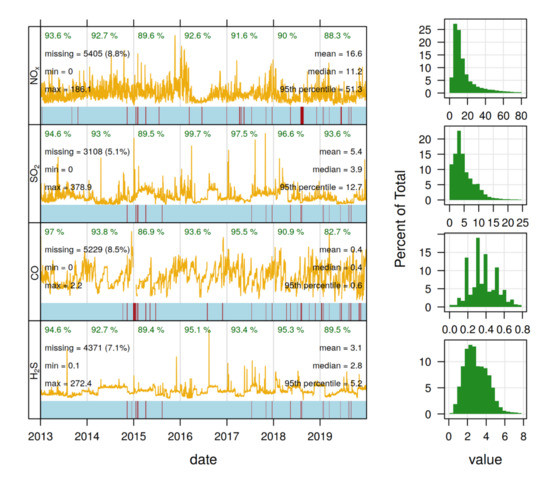
Figure 2.
Left panel: the time series data of hourly NOx, SO2, CO, H2S values (yellow lines,) and the availability and non-availability of the data (respectively the blue and red colors on the rectangular bar at the bottom of the plots). The minimum, maximum, number, and percent of missing data, mean, median and the 95th percentile for each variable plotted (in black). The percentage of the data captured for every year (in green) on the upper part of each year data plot. Right panel: the distribution of each species using a histogram plot over the selected periods.
2.3. Methodological Approach
The methodological approach to assess changes in pollutant concentrations levels, adopted in the present study, consists of 3 main steps. First, for each pollutant an RF model was built, validated, and then used to estimate the meteorologically normalized concentrations. Second, the estimation of the main change points time location in the meteorologically normalized signal and the trend analysis were performed. Third, combining the results of the previous stages with the available metadata, some hypothesis on the potential link between the step-changes in the meteorologically normalized time series and specific events were formulated.
2.3.1. RF Model Development and Meteorological Normalization Procedure
Random forest is an ML algorithm that consists of a large number of individual decision trees operating as an ensemble. Each decision tree is built on a randomly sampled subset of data and predictors and the final output of the ensemble is computed by averaging the outputs of each single tree. Deeper theoretical insight can be found in [41]. The choice of the RF algorithm in performing the meteorological normalization is due to its high accuracy in predictions, low over-fitting, reduced tuning requirements, ability to capture complex interactions and to handle highly nonlinear data [42]. In the development of the RF model, the pollutant included in the dataset represented the dependent variable (target) while meteorological and time-dependent features represented the explanatory variables (predictors). The 80% of the whole observed dataset randomly sampled (training dataset) was used to build up the prediction model. The remaining 20% (testing dataset) was used to test the prediction accuracy of the model. The performances of the RF model were assessed by comparing the observed pollutants concentrations values with those predicted by the selected model by means of a set of statistical indicators [43] evaluated on the testing dataset (cf. S1 e Table S1 in Supplementary Materials for further details). The tuning parameters of the RF model were the number of predictors randomly sampled to determine each split (mtry) and the minimum number of observations in a terminal node (min node size). The number of trees (n trees) was set at 1000. The best values of the parameters were selected minimizing the mean square error (MSE) of the difference between the predicted values and the observed ones. Moreover, the interpretability of the model was analyzed to ensure its reliability through the variable importance tool. The RF models have an inherent procedure producing the relative importance of predictors that is, the measure of the impact of each feature on the accuracy of the model. This allows identifying the most important predictors, showing their impacts on the observations, and justifying their inclusion in the model.
The meteorological normalization was carried out according to the work described in [16], as subsequently implemented in [44] and [45]. The basic idea mainly consists in developing an RF model to predict pollutant concentrations as a function of meteorological and other time variables. If the model explains an adequate amount of variance in the predicted air quality variable, it can be used to predict pollutant concentrations as a function of randomly sampled meteorological variables. The RF predictive algorithm is repeated several times (300) and the meteorologically normalized concentrations are obtained by averaging these predictions. The advantage of this procedure is that the normalization process involves only the weather conditions but not the seasonal or weekly variations, so that the resulting meteorologically normalized series is more closely related to emissions changes rather than changes due to meteorological effects.
2.3.2. Structural Change and Trend Analysis
After the meteorological normalization, a joint examination of both the change points and trend in the normalized signal was adopted. Indeed, it is worth noting that analyzing only the change points and overlooking the trend or vice versa could lead to misleading results: for example, the overall trend could mask an abrupt change in a time series of pollutant concentrations, while the trend computed between different change points could mask the overall trend [46].
In the context of the present study, the Wild Binary Segmentation (wbs) change points detection method [47] was adopted. This choice is motivated by the wbs’s ability to determine the number and potential locations of change points in the normalized concentrations time series without prior assumptions and without leading to a significant increase in computational complexity [48]. The wbs method basically uses the idea of computing cumulative sum (CUSUM) from randomly drawn intervals; the largest CUSUM is considered to be the first change points candidate to test against the stopping criteria, then this process is repeated for all the samples. More details of the theoretical aspects concerning these methods can be found in [47].
The goal of determining if there is a trend over time in the normalized concentrations was achieved using the Theil-Sen regression technique, which calculates the slopes of all possible pairs of pollutant concentrations and selects the median value [49]. The Theil-Sen method was chosen because it can be computed efficiently, it is insensitive to outliers, can be significantly more accurate than the simple linear regression method for non-normal distributed data and heteroscedasticity. In our calculations, the trends were based on monthly averages, and they were adjusted for seasonal variations, as these can have a significant effect on monthly data.
2.3.3. Metadata Analysis
Finally, in order to formulate some hypothesis on the potential link between the step-changes in the normalized time series and specific events, the available and appropriate metadata concerning plant operation, the timing of significant events related to the plant activities and the traffic flows in the Agri Valley were acquired. The former 2 were downloaded from the official website of the Italian company that manages the plant, i.e., Ente Nazionale Idrocarburi (ENI) [50], where a list of the news concerning their activity in the Basilicata Region can be consulted starting from 2016. From this list, it is possible to become aware of determinate events, such as the closing/restarting of the COVA plant, maintenance activities and gas flaring occurrences. Instead, the information on the traffic flows of the national road SS598, that is the average hourly trend and the average number of heavy and light vehicles per day, related to the years 2018–2021, were directly provided by ANAS SpA, the national company managing the Italian road and motorways network. The ANAS SpA also makes available on its official website the traffic data concerning the average daily traffic per year for heavy and light vehicles, respectively [51].
All data loading, processing, analysis, statistical modelling, and visualization were performed in the R version 4.1.0 (R Foundation for Statistical Computing, Vienna, Austria). It mainly used the Openair package for air quality and trend analysis [52], the rmweather package [53] for the meteorological normalisation, with the underlying ranger package [54] and tuneRanger package [55] for the development and tuning of the RF model, and the wbs package [56] for the change points analysis.
3. Results and Discussion
3.1. Preliminary Statistical Analysis
The descriptive statistics per year and pollutants are reported in Table 1.

Table 1.
Statistical summary of hourly concentrations of NOX, SO2, CO, H2S registered at the VZI monitoring station from January 2013 to December 2019. Mean concentration and, in rounded brackets, the min. and maximum values.
For regulated pollutants there is a general compliance with the limits set by the existing national [57] and European legislation [33]. It is worth noting that, for the sole Agri Valley, a regional law [58] identifies limit values more stringent than those in force at the national level for SO2 and H2S, since they are considered markers of the hydrocarbon emissive processes occurring in the area. This law sets at 280 μg/m3 and 100 μg/m3 the hourly and daily limit values for the protection of human health for SO2, and 32 μg/m3 the daily limit for H2S. The hourly limit value for SO2 rarely exceeded these limits and each time in different years. Overall, except for sporadic exceptions mainly related to ozone and particulate matter, the regulated pollutants showed a general compliance with the current legal limit values [59].
As far as the climate is concerned, the cold and rainy winters as well as cool summers with frequent rainfall [31], typically registered in the area, define an area at sub-continental climate. Based on the analysis of the wind data, the mean value of the ws was 1.8 ms−1, with the higher values generally measured during daytime. The wind rose on the map in Figure 1 showed a prevailing wind direction from the SW to NW sector, over the period ranging between January 2013 and December 2019. During the study period, the mean temperature was 13.78 °C, the mean relative humidity was 71.1%, while the pressure was rather static.
3.2. RF Models Development and Performances
The RF model, trained with the selection of the tuning parameters listed in Table 2, took the form shown by Equation (1) for each examined pollutant:
where rf is the function implementing the RF algorithm in the R software environment.
Table 2.
RF model tuning parameters for each of the selected pollutants.
The predictive performances and behavior of the RF models were evaluated through the statistical indicators listed in Supplementary Materials Table S1, whose resulting values were summarized in Table 3.
Table 3.
Statistical indicators of RF model performances for the testing dataset. Legend: R2 = coefficient of determination, MBE = mean bias error, MAE = mean absolute error, RMSE = root mean square error and IoA = index of agreement.
The error metrics imply that the predictions of the RF model were acceptable for all pollutants; in particular, the low MBE values indicated that there are no significant over/under estimations in the predictions. The R2 values showed that the RF models explain about 70% of the total NOx, CO and H2S variability. The low performance for SO2 (R2 values of 0.46) instead, indicated that meteorology and time variables may not be sufficient in explaining the most part of the variability in the observed SO2 data, and that there might be other variables significantly affecting SO2 concentrations.
The relative importance of the selected predictors for each of the pollutants examined is presented in Figure 3. The overall contribution of the top four predictors explained over 85% of the variance for NOX and SO2, and over 90% of the variance for CO and H2S. For SO2, CO and H2S, the temporal variables, i.e., trend and jday, were the most important predictors, indicating in the trend and seasonality the strongest driving features [60]. Since the trend captures long-term changes in the source of emissions while jday represents emissions that varies seasonally, their importance suggested that the SO2, CO and H2S variability is dominated by both the COVA plant emissions and local emissions varying over the course of the year.

Figure 3.
Relative importance of predictors for (a) NOx, (b) SO2, (c) CO and (d) H2S.
The most important contribution to the NOX varbiability, instead, was due to the wind direction, closely followed by trend, and to a lesser extent by ws and jday. Therefore, it is worth looking more closely to the dependence of NOX from wd. The bivariate polar plot (Figure 4a), showing how measured NOX hourly concentrations vary by wind speed and wind direction, depicted a strong directionality of NOX concentrations associated to winds from WSW, that is in the direction of both several of the COVA plant conveyed emissive sources and the SS598 national road. The hypothesis of a traffic contribution to NOX was supported by the analysis of the daily and weekly NOX pattern (Figure 4b,c). The former tends to be significantly bimodal (higher concentrations in the early morning and late afternoon coinciding with the commuting hour). The latter shows a clear decrease of NOX concentrations on Saturday and Sunday when traffic is usually lower. Both these patterns were also confirmed by the analysis of the metadata concerning the traffic flows of cars and heavy vehicles for the national road SS598 provided by ANAS (Figure 4d).
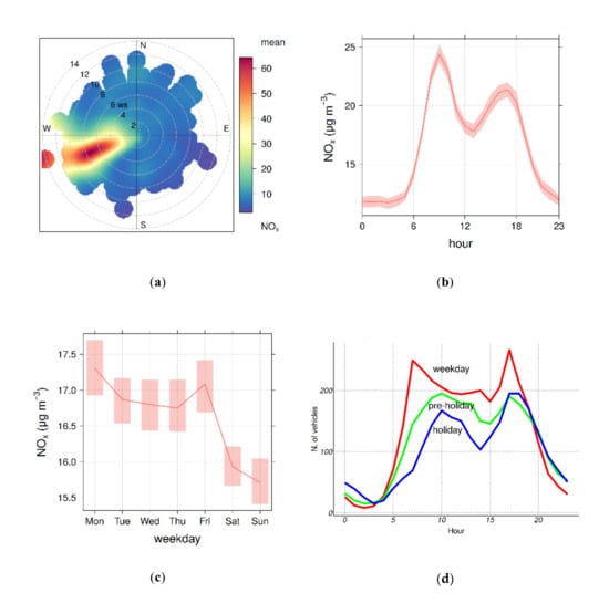
Figure 4.
Polar plot (a), daily (b) and weekly (c) profiles of hourly NOX concentrations over the 2013–2019 period. Also shown on the plots (b) and (c) is the 95% confidence interval in the mean. (d) Average hourly trend of traffic flows of the national road SS598 in 2019.
Moreover, although for SO2 and H2S, wd is of much less relative importance, the polar plots in Figure S2a,b of the Supplementary Materials showed approximately the same directionality from the W, S–W sector, confirming the common sources origin of these pollutants. More ambiguous, instead, is the contribution of wd to the CO levels (Figure S2c in the Supplementary Materials). This can be due to the presence of several different sources of CO in the area other than the COVA plant and traffic, such as combustion processes related to agricultural activities, as suggested in [35].
Overall, the above showed that, although the data-driven approach here adopted do not consider the physical and chemical processes underlying the air pollution variability, the model results were plausible and indirectly confirmed by others’ independent evidence.
3.3. Meteorological Normalization, Change Points and Trend Analysis
Daily concentrations of the observed and meteorologically normalized data for NOX, SO2, CO and H2S are shown in Figure 5 and Figure 6 (respectively red dots and green line). The blue solid line represents instead the line joining the main 14 change points detected using the wbs algorithm and summarized in Table S2 of the Supplementary Materials for each pollutant.
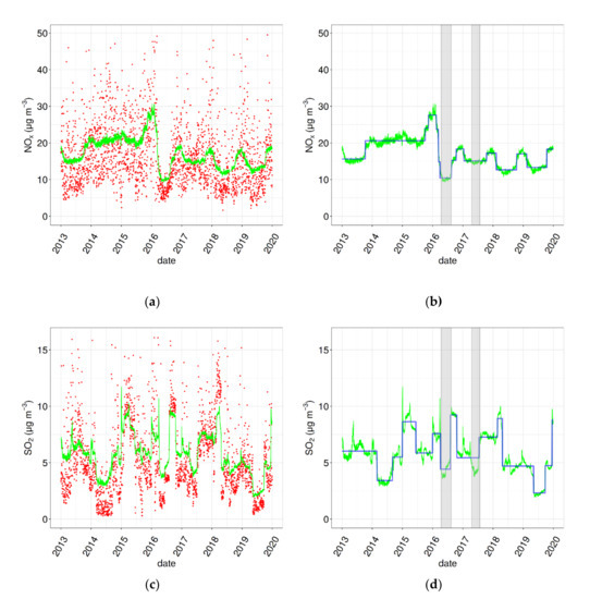
Figure 5.
(a,c): daily averages of observed (red dots) and meteorologically normalized (green lines) NOx and SO2 concentrations. (b,d) the wbs change points (blue lines) and the periods of COVA plant shutdowns (grey areas).
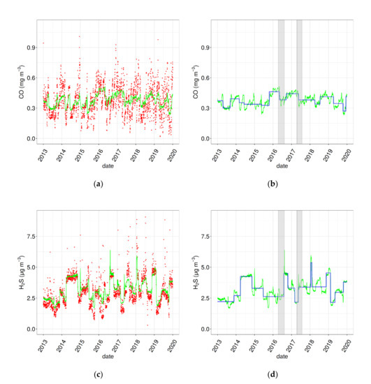
Figure 6.
(a,c) daily averages of observed (red dots) and meteorologically normalized (green lines) CO and H2S concentrations. (b,d) the wbs change points (blue lines) and the periods of COVA plant shutdowns (grey areas).
As result of the meteorological normalization process, clear differences can be seen between the observed and normalized concentrations with the latter being a much smoother data series, as illustrated in Figure 5a,c for NOX and SO2 and Figure 6a,c for CO and H2S. The normalized pollutants concentrations time series were less noisy compared to the observed values so allowing revealing the influence of changes in emissions to the pollution level measured at the examined site. Applying the wbs method on the normalized signal, number and location of change points were identified to highlight the main structural changes in the time series of pollutants concentrations. Once these structural changes were identified, it was possible to try to link them to known events through the available metadata. In this regard, it is worth dwelling on two specific events, corresponding to the periods represented by the grey areas in Figure 5b,d for NOX and SO2 and Figure 6b,d for CO and H2S, for which public metadata are available. Indeed, by means of the information obtainable through the ENI web site [45], it is known that the first period, from March to August 2016, corresponds to a COVA plant shutdown in the context of a judicial investigation on the disposal of liquid waste produced by the exploration and pre-treatment of hydrocarbon activities.
The second one, from April to July 2017, consists of another plant shutdown due to a major accident caused by the release of hydrocarbons from a storage unit. As far as the SO2 and CO signals are concerned, a decrease in concentrations corresponding to these periods can be observed in Figure 5d and Figure 6b. With respect to the NOX pollutant, a strong correspondence was found between the normalized concentrations trend and the event which occurred at the COVA plant in 2016, Figure 5b. The lack of correspondence with the event registered in 2017 may be due to other sources contributing to the observed NOX level. As shown in Figure 6d, H2S, instead, seems to be less affected by these closure periods, as expected, since this pollutant is representative of the diffuse emissions of the COVA plant, which plausibly persist even during periods of plant shutdown.
The examples above illustrated seem to confirm the goodness of the developed approach in identifying and explaining an atmospheric response in the observed data after an unplanned event or a change in emission sources. However, further and independent verification to confirm the various hypotheses are always desirable if not necessary, given the extreme complexity of the phenomena considered.
Finally, Table 4 summarizes the results of the Theil-Sen regression analysis. Both emissions and meteorological changes contribute to the observed trends of pollutant concentrations, while in the normalized trend the influence of meteorological changes is disentangled. For NOX, a statistically significant trend was found for both normalized and observed data (p < 0.001), while less statistically significant trends were found for H2S and CO (p < 0.05) and SO2 (p < 0.1). Overall, the comparison between the observed and normalized slopes for each pollutant showed a generally scarce influence of the weather conditions on the trend of the pollutants. On the other hand, the low relevance of the weather conditions is consistent with the information deduced from the results illustrated above, which indicate in the local anthropic NOX sources the main drivers of NOX variability.
Table 4.
Theil-Sen slope and 95% confidence intervals of the observed and meteorologically normalized pollutants concentrations. The symbols shown next to the square bracket relate to how statistically significant the trend estimate is: p < 0.001 = ***, p < 0.05 = * and p < 0.1 = +.
Given the statistically significant trend observed for the NOx signal, a deeper joined analysis of the Theil-Sen trend with the change points detection was carried out. To this end, the meteorological normalized NOX data were divided into two segments, based on the main change point as detected by the wbs method. Both segments were then analyzed for the presence of trend and compared with the trend predicted when the whole dataset is considered. According to the results shown in Figure 7a, a downward trend is observed when the whole dataset is analyzed. The other way around, when we divide the dataset into two segments and test them before and after the main change point, an increasing trend can be observed in the first part and no trend in the second part of the data (Figure 7b,c, respectively). In other words, assessing the overall trend on the whole dataset without taking into account the main change point, the sharp change in the data in March of 2016 is obscured. The same trend analysis carried out on the observed data gave similar results. However, it is worth mentioning that analyzing a signal from which the weather effect has been removed allows better highlighting of the other causes that determine the changes in the signal. This example shows how the proposed approach could help in the right attribution of changes in pollutant levels to specific events, and consequently in the assessment of the effectiveness of the air quality interventions.
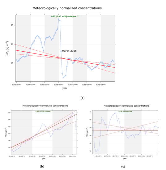
Figure 7.
Trend analysis for (a) the NOX complete normalized series, (b) before and (c) after the main change point. Plots show deseasonalized monthly mean concentrations of NOX. Solid red line shows trend estimate and dashed red shows 95% confidence intervals.
4. Conclusions
In the present paper a procedure combining change points, trend analysis and metadata has been illustrated to assess and explain the changes in pollutant concentrations levels once the confounding effects of weather have been accounted for with ML-RF models. The practical application of the procedure allowed linking the step-changes in the NOx pollutant concentrations to a specific event related to the existing anthropic sources.
However, since the meteorological normalization process adopted in the developed procedure is based on data-driven models, caution is required when generalizing the results obtained to different conditions and/or sites. Moreover, strong interaction with the local environmental and health authorities is desirable to widen the knowledge on the features and the criticalities of the examined area.
Overall, our results show that the adopted procedure can improve the assessment of observed air pollutants data and help in revealing shifts in pollutants levels that cannot be clearly seen in the original data, so providing significant information for the implementation of effective strategies to prevent the health impact of air pollution.
Supplementary Materials
The following supporting information can be downloaded at: https://www.mdpi.com/article/10.3390/atmos13010064/s1, Table S1 summarizes name and equation of the statistical indicators; Figure S1 summarizes main statistical aspects of the meteorological parameters; Figure S2 illustrates the polar plots for SO2, CO and H2S; Table S2 lists the main 14 change points detected for each examined pollutant.
Author Contributions
Conceptualization, R.V.G. and C.A.; methodology, R.V.G. and C.A.; software, R.V.G.and C.A.; validation, R.V.G. and C.A.; formal analysis, R.V.G. and C.A.; investigation, R.V.G. and C.A.; resources, R.V.G. and C.A.; data curation, R.V.G. and C.A.; writing—original draft preparation, R.V.G. and C.A.; writing—review and editing, R.V.G. and C.A.; visualization, R.V.G. and C.A. All authors have read and agreed to the published version of the manuscript.
Funding
This research received no external funding.
Data Availability Statement
Publicly available datasets were analyzed in this study. The measurements from the ARPA Basilicata air quality network can be found on the web page http://www.arpab.it/opendata/q_aria_serie.asp (accessed on 1 October 2019) Traffic data can be found on the web page https://www.stradeanas.it/it/le-strade/osservatorio-del-traffico/dati-traffico-medio-giornaliero-annuale accessed on (2 December 2019).
Acknowledgments
The authors are grateful to the Environmental Protection Agency of Basilicata Region and ANAS for providing the data used in this work.
Conflicts of Interest
The authors declare no conflict of interest.
References
- World Health Organization. WHO Global Air Quality Guidelines: Particulate Matter (PM2.5 and PM10), Ozone, Nitrogen Dioxide, Sulfur Dioxide and Carbon Monoxide; World Health Organization: Geneva, Switzerland, 2021; ISBN 978-92-4-003422-8. [Google Scholar]
- Public Health England. Review of Interventions to Improve Outdoor Air Quality and Public Health; PHE Publications: London, UK, 2019. [Google Scholar]
- Henneman, L.R.F.; Liu, C.; Mulholland, J.A.; Russell, A.G. Evaluating the Effectiveness of Air Quality Regulations: A Review of Accountability Studies and Frameworks. J. Air Waste Manag. Assoc. 2017, 67, 144–172. [Google Scholar] [CrossRef]
- Air Quality Expert Group. Assessing the Effectiveness of Interventions on Air Quality; Department for Environment, Food and Rural Affairs, Scottish Government, Welsh Government and Department of Agriculture, Environment and Rural Affairs in Northern Ireland, 2020. Available online: https://ukair.defra.gov.uk/assets/documents/reports/cat09/2006240803_Assessing_the_effectiveness_of_Interventions_on_AQ.pdf (accessed on 26 August 2021).
- Pérez, I.A.; García, M.Á.; Sánchez, M.L.; Pardo, N.; Fernández-Duque, B. Key Points in Air Pollution Meteorology. Int. J. Environ. Res. Public Health 2020, 17, 8349. [Google Scholar] [CrossRef]
- Henneman, L.R.F.; Holmes, H.A.; Mulholland, J.A.; Russell, A.G. Meteorological Detrending of Primary and Secondary Pollutant Concentrations: Method Application and Evaluation Using Long-Term (2000–2012) Data in Atlanta. Atmos. Environ. 2015, 119, 201–210. [Google Scholar] [CrossRef]
- Kinney, P.L. Climate Change, Air Quality, and Human Health. Am. J. Prev. Med. 2008, 35, 459–467. [Google Scholar] [CrossRef]
- Thompson, M.L.; Reynolds, J.; Cox, L.H.; Guttorp, P.; Sampson, P.D. A Review of Statistical Methods for the Meteorological Adjustment of Tropospheric Ozone. Atmos. Environ. 2001, 35, 617–630. [Google Scholar] [CrossRef]
- Wise, E.K.; Comrie, A.C. Extending the Kolmogorov–Zurbenko Filter: Application to Ozone, Particulate Matter, and Meteorological Trends. J. Air Waste Manag. Assoc. 2005, 55, 1208–1216. [Google Scholar] [CrossRef]
- Akpinar, E.; Akpinar, S.; Öztop, H. Statistical Analysis of Meteorological Factors and Air Pollution at Winter Months in Elaziğ, Turkey. J. Urban Environ. Eng. 2009, 3, 7–16. [Google Scholar] [CrossRef]
- Gardner, M.; Dorling, S. Artificial Neural Network-Derived Trends in Daily Maximum Surface Ozone Concentrations. J. Air Waste Manag. Assoc. 2001, 51, 1202–1210. [Google Scholar] [CrossRef]
- Doreswamy, K.S.H.; Km, Y.; Gad, I. Forecasting Air Pollution Particulate Matter (PM2.5) Using Machine Learning Regression Models. Procedia Comput. Sci. 2020, 171, 2057–2066. [Google Scholar] [CrossRef]
- Grange, S.K.; Carslaw, D.C.; Lewis, A.C.; Boleti, E.; Hueglin, C. Random Forest Meteorological Normalisation Models for Swiss PM10 Trend Analysis. Atmos. Chem. Phys. 2018, 18, 6223–6239. [Google Scholar] [CrossRef]
- Petetin, H.; Bowdalo, D.; Soret, A.; Guevara, M.; Jorba, O.; Serradell, K.; Pérez García-Pando, C. Meteorology-Normalized Impact of COVID-19 Lockdown upon NO2 Pollution in Spain. Atmos. Chem. Phys. 2020, 20, 11119–11141. [Google Scholar] [CrossRef]
- Gagliardi, R.V.; Andenna, C. Machine Learning Meteorological Normalization Models for Trend Analysis of Air Quality Time Series. Int. J. EI 2021, 4, 375–389. [Google Scholar] [CrossRef]
- Grange, S.K.; Carslaw, D.C. Using Meteorological Normalisation to Detect Interventions in Air Quality Time Series. Sci. Total Environ. 2019, 653, 578–588. [Google Scholar] [CrossRef] [PubMed]
- Xiong, L.; Guo, S. Trend Test and Change-Point Detection for the Annual Discharge Series of the Yangtze River at the Yichang Hydrological Station/Test de Tendance et Détection de Rupture Appliqués Aux Séries de Débit Annuel Du Fleuve Yangtze à La Station Hydrologique de Yichang. Hydrol. Sci. J. 2004, 49, 99–112. [Google Scholar] [CrossRef]
- Guerreiro, C.B.B.; Foltescu, V.; de Leeuw, F. Air Quality Status and Trends in Europe. Atmos. Environ. 2014, 98, 376–384. [Google Scholar] [CrossRef]
- Chen, J.; Gupta, A.K. Parametric Statistical Change Point Analysis; Birkhäuser: Boston, MA, USA, 2012; ISBN 978-0-8176-4800-8. [Google Scholar]
- Huang, H.; Wang, Z.; Xia, F.; Shang, X.; Liu, Y.; Zhang, M.; Dahlgren, R.A.; Mei, K. Water Quality Trend and Change-Point Analyses Using Integration of Locally Weighted Polynomial Regression and Segmented Regression. Environ. Sci. Pollut. Res. 2017, 24, 15827–15837. [Google Scholar] [CrossRef]
- Jaiswal, R.K.; Lohani, A.K.; Tiwari, H.L. Statistical Analysis for Change Detection and Trend Assessment in Climatological Parameters. Environ. Process. 2015, 2, 729–749. [Google Scholar] [CrossRef]
- Suhaila, J.; Yusop, Z. Trend Analysis and Change Point Detection of Annual and Seasonal Temperature Series in Peninsular Malaysia. Meteorol. Atmos. Phys. 2018, 130, 565–581. [Google Scholar] [CrossRef]
- Nguyen, K.N.; Quarello, A.; Bock, O.; Lebarbier, E. Sensitivity of Change-Point Detection and Trend Estimates to GNSS IWV Time Series Properties. Atmosphere 2021, 12, 1102. [Google Scholar] [CrossRef]
- Garcia-Gonzales, D.A.; Shonkoff, S.B.C.; Hays, J.; Jerrett, M. Hazardous Air Pollutants Associated with Upstream Oil and Natural Gas Development: A Critical Synthesis of Current Peer-Reviewed Literature. Annu. Rev. Public Health 2019, 40, 283–304. [Google Scholar] [CrossRef] [PubMed]
- European Commission, Directorate General for Health and Food Safety. Opinion on the Public Health Impacts and Risks Resulting from Onshore Oil and Gas Exploration and Exploitation in the EU; Publications Office: Luxembourg, 2018. [Google Scholar]
- Johnston, J.E.; Lim, E.; Roh, H. Impact of Upstream Oil Extraction and Environmental Public Health: A Review of the Evidence. Sci. Total Environ. 2019, 657, 187–199. [Google Scholar] [CrossRef]
- Granella, F.; Aleluia Reis, L.; Bosetti, V.; Tavoni, M. COVID-19 Lockdown Only Partially Alleviates Health Impacts of Air Pollution in Northern Italy. Environ. Res. Lett. 2021, 16, 035012. [Google Scholar] [CrossRef]
- Diémoz, H.; Magri, T.; Pession, G.; Tarricone, C.; Tombolato, I.K.F.; Fasano, G.; Zublena, M. Air Quality in the Italian Northwestern Alps during Year 2020: Assessment of the COVID-19 «Lockdown Effect» from Multi-Technique Observations and Models. Atmosphere 2021, 12, 1006. [Google Scholar] [CrossRef]
- ENI-In Val d’Agri Con Le Attività Upstream. Available online: https://www.eni.com/it-IT/attivita/italia-val-agri-attivita-upstream.html (accessed on 11 January 2021).
- Faruolo, M.; Coviello, I.; Filizzola, C.; Lacava, T.; Pergola, N.; Tramutoli, V. A Satellite-Based Analysis of the Val d’Agri Oil Center (Southern Italy) Gas Flaring Emissions. Nat. Hazards Earth Syst. Sci. 2014, 14, 2783–2793. [Google Scholar] [CrossRef]
- Prefettura Di Potenza-PEE Centro Olio Val d’Agri Di Viggiano-Edizione 2013. Available online: http://www.prefettura.it/potenza/contenuti/Pee_centro_olio_val_d_agri_di_viggiano_edizione_2013-64403.htm (accessed on 30 March 2021).
- Gobbi, G.P.; Barnaba, F.; Di Liberto, L.; Bolignano, A.; Lucarelli, F.; Nava, S.; Perrino, C.; Pietrodangelo, A.; Basart, S.; Costabile, F.; et al. An Inclusive View of Saharan Dust Advections to Italy and the Central Mediterranean. Atmos. Environ. 2019, 201, 242–256. [Google Scholar] [CrossRef]
- European Commission. DIRECTIVE 2008/50/EC on ambient air quality and cleaner air for Europe. Off. J. Eur. Union 2008, L152/1, 1–44. [Google Scholar]
- ARPAB-Inquinanti Monitorati. Available online: http://www.arpab.it/aria/inquinanti.asp (accessed on 5 March 2021).
- Calvello, M.; Esposito, F.; Trippetta, S. An Integrated Approach for the Evaluation of Technological Hazard Impacts on Air Quality: The Case of the Val d’Agri Oil/Gas Plant. Nat. Hazards Earth Syst. Sci. 2014, 14, 2133–2144. [Google Scholar] [CrossRef][Green Version]
- ARPAB-Gli Open Data- Qualità Dell’aria. Available online: www.arpab.it/opendata/q_aria_serie.asp (accessed on 11 January 2021).
- Regione Basilicata–Valutazione Ambientale. Available online: http://valutazioneambientale.regione.basilicata.it/valutazioneambie/home.jsp (accessed on 10 February 2021).
- WHO-Air Quality and Health. Available online: https://www.who.int/teams/environment-climate-change-and-health/air-quality-and-health/health-impacts (accessed on 11 January 2021).
- Mangia, C. Modeling Air Quality Impact of Pollutants Emitted by an Oil/Gas Plant in Complex Terrain in View of a Health Impact Assessment. Air Qual. Atmos. Health 2019, 12, 491–502. [Google Scholar] [CrossRef]
- Mousa, H.A.-L. Short-Term Effects of Subchronic Low-Level Hydrogen Sulfide Exposure on Oil Field Workers. Environ. Health Prev. Med. 2015, 20, 12–17. [Google Scholar] [CrossRef]
- Breiman, L. Statistical Modeling: The Two Cultures. Stat. Sci. 2001, 16, 199–215. [Google Scholar] [CrossRef]
- Ameer, S.; Shah, M.A.; Khan, A.; Song, H.; Maple, C.; Islam, S.U.; Asghar, M.N. Comparative Analysis of Machine Learning Techniques for Predicting Air Quality in Smart Cities. IEEE Access 2019, 7, 128325–128338. [Google Scholar] [CrossRef]
- Sayegh, A.S.; Munir, S.; Habeebullah, T.M. Comparing the Performance of Statistical Models for Predicting PM10 Concentrations. Aerosol Air Qual. Res. 2014, 14, 653–665. [Google Scholar] [CrossRef]
- Vu, T.V.; Shi, Z.; Cheng, J.; Zhang, Q.; He, K.; Wang, S.; Harrison, R.M. Assessing the Impact of Clean Air Action on Air Quality Trends in Beijing Using a Machine Learning Technique. Atmos. Chem. Phys. 2019, 19, 11303–11314. [Google Scholar] [CrossRef]
- Shi, Z.; Song, C.; Liu, B.; Lu, G.; Xu, J.; Van Vu, T.; Elliott, R.J.R.; Li, W.; Bloss, W.J.; Harrison, R.M. Abrupt but Smaller than Expected Changes in Surface Air Quality Attributable to COVID-19 Lockdowns. Sci. Adv. 2021, 7, eabd6696. [Google Scholar] [CrossRef] [PubMed]
- Sharma, S.; Swayne, D.A.; Obimbo, C. Trend Analysis and Change Point Techniques: A Survey. Energ. Ecol. Environ. 2016, 1, 123–130. [Google Scholar] [CrossRef]
- Fryzlewicz, P. Wild Binary Segmentation for Multiple Change-Point Detection. Ann. Statist. 2014, 42, 2243–2281. [Google Scholar] [CrossRef]
- Aminikhanghahi, S.; Cook, D.J. A Survey of Methods for Time Series Change Point Detection. Knowl. Inf. Syst. 2017, 51, 339–367. [Google Scholar] [CrossRef]
- Nunifu, T.K.; Fu, L. Methods and Procedures for Trend Analysis of Air Quality Data; Government of Alberta, Ministry of Environment and Parks: Alberta, Canada, 2019; Available online: https://open.alberta.ca/publications/9781460136379 (accessed on 15 January 2021)ISBN 9781460136379.
- ENI in Basilicata. Available online: https://www.eni.com/eni-basilicata/news/2021-elenco-news.page (accessed on 11 January 2021).
- ANAS-Le Strade. Available online: https://www.stradeanas.it/it/strade (accessed on 11 January 2021).
- Carslaw, D.; Ropkins, K. Openair-An R package for air quality data analysis. Environ. Model. Softw. 2012, 27, 52–61. [Google Scholar] [CrossRef]
- Grange, S.K.; Tools to Conduct Meteorological Normalisation on Air Quality Data. Tools to Conduct Meteorological Normalisation on Air Quality Data. Available online: https://github.com/skgrange/rmweather (accessed on 11 January 2021).
- Wright, M.N.; Ziegler, A. Ranger: A Fast Implementation of Random Forests for High Dimensional Data in C++ and R. J. Stat. Softw. 2017, 77. [Google Scholar] [CrossRef]
- Probst, P.; Wright, M.; Boulesteix, A.-L. Hyperparameters and Tuning Strategies for Random Forest. WIREs Data Min. Knowl. Discov. 2019, 9, e1301. [Google Scholar] [CrossRef]
- Baranowski, R.; Fryzlewicz, P.; Wbs: Wild Binary Segmentation for Multiple Change-Point Detection. R wbs Package Version 1.4. 2019. Available online: https://cran.r-project.org/web/packages/wbs/wbs.pdf (accessed on 5 November 2021).
- Decreto Legislativo n. 155/10, Attuazione della Direttiva 2008/50/CE relativa alla qualità dell’aria ambiente e per un’aria più pulita in Europa. Gazz. Uff. 2010, 216, 1–111.
- Norme Tecniche Ed Azioni per La Tutela Della Qualità Dell’aria Nei Comuni Di Viggiano e Grumento Nova. In Proceedings of the Delibera Giunta Regione Basilicata n. 983, Basilicata, Italy, 6 August 2013.
- ARPAB-Arpa Informa: Pubblicazioni. Rapporto Annuale dei Dati Ambientali 2019. Available online: www.arpab.it/pubblicazioni.asp (accessed on 10 January 2020).
- Falocchi, M.; Zardi, D.; Giovannini, L. Meteorological Normalization of NO2 Concentrations in the Province of Bolzano (Italian Alps). Atmos. Environ. 2021, 246, 118048. [Google Scholar] [CrossRef]


Publisher’s Note: MDPI stays neutral with regard to jurisdictional claims in published maps and institutional affiliations. |
© 2021 by the authors. Licensee MDPI, Basel, Switzerland. This article is an open access article distributed under the terms and conditions of the Creative Commons Attribution (CC BY) license (https://creativecommons.org/licenses/by/4.0/).