Abstract
In this study, National Centers for Environmental Prediction (NCEP) Final (FNL) operational global analysis data and meteorological observation data from 2013 to 2017 were used to evaluate the impact of seasonal changes and different circulation classifications on the dynamical downscaling simulation results of Weather Research and Forecasting (WRF) in the Pearl River Delta (PRD) region. The results show that the dynamical downscaling method can accurately simulate the time variation characteristics of the near-surface meteorological field and the hit rates of a 2-m temperature, 2-m relative humidity, 10-m wind speed, and 10-m wind direction are 92.66%, 93.98%, 26.78%, and 76.78%, respectively. The WRF model slightly underestimates the temperature and relative humidity, and overestimates the wind speed and precipitation. For precipitation, the WRF model can better simulate the variation characteristics of light rain and heavy rain, with the probability of detection are 0.59 and 0.69, respectively. For seasonal factors, the WRF model can conduct a perfect simulation in autumn and winter, followed by spring, while summer is vulnerable to extreme weather, so the result of the simulation is relatively poor. The circulation type is an important parameter of downscaling assessment. When the PRD is controlled by high pressure, the simulated results of WRF are good, and when the PRD is affected by low pressure or extreme weather, the simulation results are relatively poor.
1. Introduction
Global Climate Models (GCMs) may be sufficient for describing large-scale circulations and climate [1], but it is difficult for them to reproduce regional and local circulations and climate. When GCMs focus on the regional climate, they generally exhibit several problems, such as an output with a low spatial resolution, the inability to clearly describe the climate distribution difference in the basin region, and a limited ability to simulate extreme weather events. Moreover, these limitations are further amplified in areas with a complex topography, irregular coastline, and uneven soil cover, where the thermal and dynamic mechanical cycles are greatly affected by the heterogeneity of the surface.
High-resolution meteorological data are required for regional and local climate research, wind energy assessment, the hydrological and land surface model (LSM), and the land surface data assimilation system. The fifth Intergovernmental Panel on Climate Change (IPCC) report also highlighted the regional characteristics and differences of climate change, so the downscaling of regional climate data has become an urgent and promising topic [2]. Current downscaling approaches, which represent a bridge linking coarse-resolution meteorological data (e.g., reanalysis and GCMs data) and high-resolution meteorological data [3], include statistical downscaling of GCMs outputs and dynamical downscaling using RCMs (Regional Climate Models) nested with GCMs [4,5]. The basic principle of statistical downscaling is appropriate choice of transfer functions and predictor variable, determine the empirical relationship between large-scale climate elements and local climate elements, and then apply this empirical relationship to GCMs output. The advantage of statistical downscaling is less computation, which can facilitates the ensembles of climate realizations generation [6]. Dynamical downscaling based on RCMs has a clear physical basis and is unaffected by observational data. The global reanalysis data provide initial conditions and boundary conditions for RCMs. RCMs can preserve the large-scale characteristics of GCMs, and meanwhile integrate the local weather and the complex terrain information (such as mountains, coastlines, etc.) to improve the resolution of reanalysis data [1]. Dynamical downscaling needs more computer time than statistical downscaling. With the progress of computing speed, dynamic downscaling is easier to implement, and it has been widely used in the Pearl River Delta (PRD) region [7,8].
With more accurate information on land surface inhomogeneity, RCMs can reproduce the local circulation and climate well. The Weather Research and Forecasting (WRF) model includes a wide range of physical parameterizations, and various data (e.g., data from GCMs or weather prediction model and reanalysis data) can be employed as the driving field for WRF, making WRF one of the most widely used RCMs. Dynamical downscaling studies using WRF include the assessment of downscaling results, comparing results from different model resolutions, the impact of different physical parameterizations, the effect of initial conditions (e.g., sea surface and soil temperature) and large-scale circulations [9,10] on WRF simulations, ensemble methods with initial condition perturbing or different initial data to reduce the uncertainties in the initial conditions, and data assimilation research [11].
Guo et al. (2017) use a high-resolution RCMs ensemble to study the extreme precipitation in China, they found the downscaling method can better simulate the local variation characteristics of precipitation [12]. Qiu et al. (2017) use WRF to downscaling European Centre for Medium-Range Weather Forecasts Re-Analysis-Interim (ERA-interim) data, and they find the result of dynamical downscaling have overall comparable accuracy in temperature and precipitation to ERA-interim data, and are more accurate in extreme events [13]. However, the performance of dynamical downscaling displays differences in different regions and seasons [14]. Meteorological simulation faces more challenges in complex terrain regions [15,16]. The existing reanalysis data often have a low resolution, which cannot accurately reflect the changes of temperature and precipitation caused by the regional climate in areas with a complex terrain, and the description of the extreme climate state often exhibits large deviations. Therefore, the dynamical downscaling is a suitable method to obtain the characteristics of regional climate change with a higher resolution than reanalysis data.
The Pearl River Delta (PRD) is located in the south of China. With a complex terrain and distribution of land and sea, and a high degree of urbanization, local and regional circulations are complex. In this study, dynamical downscaling of the National Centers for Environmental Prediction (NCEP) Final (FNL) Operational Global Analysis data in PRD was carried out. The performance of WRF dynamical downscaling was evaluated by comparing the observation data of meteorological stations, including 2-m temperature (T2), 2-m relative humidity (RH2), 10-m wind speed (WS) and wind direction (WD), precipitation (PRE), and the extreme climate index. The impacts of season and weather conditions on WRF dynamical downscaling were investigated.
2. Data and Method
2.1. WRF Model Design
The WRF model is a next-generation mesoscale numerical weather model and has been increasingly used as RCM. The effort to develop WRF has been a collaborative partnership, principally among the National Center for Atmospheric Research (NCAR), the NCEP, and other research institutions and universities, it has two dynamical cores: Advanced Research WRF (ARW) and nonhydrostatic mesoscale model (NMM) [17]. WRF-ARW v3.8 was used in this study. Many studies discussed the impact of different physics parameterizations on dynamical downscaling [18,19]. It was difficult to determine an optimal combination of parameterization schemes [9]. The physical parameterizations used in this study were the WRF Single-Moment 6–class (WSM6) microphysics scheme, the Kain–Fritsch (KF) cumulus parameterization scheme, the Rapid Radiative Transfer Model (RRTM) longwave and Dudhia shortwave radiation parameterization scheme, the Yonsei University (YSU) planetary boundary layer parameterization scheme, and the Noah LSM parameterization scheme, which have been widely applied in PRD [20,21] and other regions [22,23].
WRF was configured so that it had two nested domains, in order to reduce the errors of boundary effects: An outer domain (D01) with a horizontal resolution of 25 km (140 × 100 grid points) covering southern China, most of the Indochina Peninsula, and the South China Sea, and an inner domain (D02) with a 5 km resolution (100 × 100 grid points) covering the Pearl River Delta (PRD) region and surrounding areas (Figure 1a). Vertically, there were a total of 35 full η levels extending to the model top at 50 hPa, with 16 levels below 2 km. The model integration covers five years from 2013 to 2017. The model simulation was re-initialized every month using a 24-h spin-up, with time-steps of 150 and 30 s for domains D01 and D02, respectively.
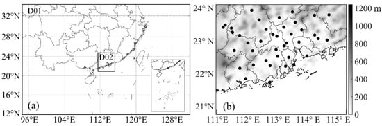
Figure 1.
Two nested domains of the Weather Research and Forecast (WRF) (a), and the terrain and 40 meteorological stations in the inner domain (b).
The WRF model relies on a driving field established by reanalysis, GCM data, and so on to provide initial lateral and surface boundary conditions for RCMs, and transmits the weather background information to RCMs. Nevertheless, for long-playing or large domain simulations, the result of the simulation by RCM may exhibit differences from the driving field. Previous studies show that there are many methods that can solve this problem, which involve frequent re-initialization, analysis nudging, spectral nudging, and scale-selective bias correction [24]. In this study, we used analysis nudging to reduce the deviation of the driving field, as some studies have pointed out that interior nudging can retain large-scale information from the driving filed and improve the model effect [10]. When the driving field is not significantly coarser than the model resolution, analysis nudging is sufficient for improving the performance of the numerical model [25].
2.2. Meteorological Data
NCEP FNL data, based on 1° × 1° available operationally every 6 h, were used as the driving filed for WRF with analysis nudging. They were obtained from the Global Data Assimilation System (GDAS), which collects observational data from the Global Telecommunications System (GTS), ground-based observations, aircraft, and satellite observations, and other sources, for many analyses.
Daily ground meteorological observation data, including T2, RH2, WS, WD, and PRE, were acquired from the National Meteorological Information Centre (NMIC) to evaluate the performance of WRF. The study area includes 40 meteorological stations. The distribution of meteorological stations is shown in Figure 1b.
Except for conventional meteorological elements, the performance of extreme weather and climate is an important indicator of successful dynamic downscaling. In the early 21st century, The World Meteorological Organization (WMO) and the World Climate Research Program (WCRP) jointly established the Climate Change Monitoring and Index Expert Group (ETCCDI), and they proposed a set of unified criteria for climate change monitoring, i.e., extreme climate indices. There are 27 extreme climate indices, including 16 extreme temperature indices and 11 extreme precipitation indices, which form the core of extreme climate indices [26]. In this study, five extreme temperature indices and five extreme precipitation indices (Table 1) were selected to further study the performance of WRF dynamic downscaling for regional extreme weather. The extreme climate indices observed were calculated based on hourly ground meteorological observation data.

Table 1.
Definitions of 10 extreme weather event indices.
2.3. Model Evaluation
Although previous studies revealed that dynamical downscaling have overall comparable accuracy in near-surface meteorological elements [13], the comparison between NCEP FNL data, WRF simulation results, and the observations is important to conclude the interest to perform downscaling with WRF. Thus, this paper simply compares the effect of WRF dynamical downscaling and NCEP FNL data.
Many dynamical downscaling studies have evaluated simulated results using gridded observations [9]. As most gridded observations have difficulty in describing the local and regional climate characteristics due to a low resolution [27], and lose some important local information when interpolated from site observations, site observations were used to evaluate the performance of WRF dynamical downscaling.
There are some uncertainties when directly comparing model outputs with observations as modeled variables represent the average in a model grid, while observations represent the state at a specific point. However, it is difficult to solve the problem at present. On the other hand, the dominant (e.g., land use and soil type) or average (e.g., topography and vegetation fraction) land surface properties are used in a model grid and land surface properties are smoothed by horizontal spatial discretization, so the nearest grid point may not be the most suitable one for representing the observations, resulting in “representativeness error” [28]. “Representativeness error” is not the focus of this paper, and the error was treated in a simple way in this study. We use Nearest Neighbor Interpolation to choose the nearest grid point to the observation stations was selected to evaluate the performance of WRF. A correction of the daily average temperature was made using a constant lapse rate of 6 K km−1 to compensate for the elevation differences between the observation site and the nearest model grid [29]. No corrections were applied to other meteorological elements due to the complex relationships between them and land surface properties.
Six standard statistical indices: the correlation coefficient (R), the root mean square error (RMSE), the hit rate (HR), the standard deviation (STD), the index of agreement (IA), and the mean bias (MB), were used for model evaluation [30]. The selection of HR is related to the standard value, and the criteria values of HR for T2, RH2, WS, and WD are 2 °C, 10%, 1 m s−1, and 30° [23]. For PRE, another three classified statistical indices, including the probability of detection (POD), the false alarm rate (FAR), and the Heidke skill score (HSS), are used to verify a forecast against an observation of a binary event (yes or no). POD and FAR values vary between 0 and 1, and HSS values vary between −1 and 1. The ideal POD, FRA, and HSS are 1, 0, and 1, respectively [31]. The formulae for these statistical parameters are shown in Table 2.
Table 2.
The formulae of standard statistical indices employed in this study.
However, there is no clear domestic or foreign criterion about how the size of these values indicates the reliability of the simulation results. Some researchers have pointed out in evaluations of simulation studies on ground elements that when IA is relatively large, RMSE < STDo and STDo is relatively close to STDf, and the mean simulation or prediction results are considered to be more reliable [32].
2.4. Circulation Classification
The impact of the circulation type on WRF dynamical downscaling is an important research object in this study. The circulation type can be classified by the grid data of the sea level pressure, potential height, or wind field. At present, there are five commonly used classification methods, which are correlation methods, cluster analysis, principal component analysis, the fuzzy method, and the nonlinear method [23], and this study is based on European Centre for Medium-Range Weather Forecasts (ECMWF) ERA-Interim sea level pressure re-analysis data collected at 08:00 Beijing time every day during 2013 to 2017. T-mode principal component analysis (PCA) combined with the K-means cluster approach was used to identify circulation types, and this method has been widely used in previous studies [33]. According to the criterion function, nine circulation types (CT1–CT9) were identified (Figure 2).
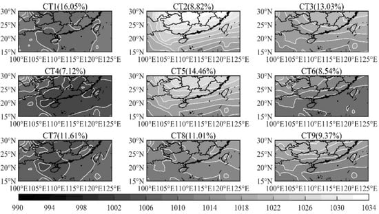
Figure 2.
The mean sea level pressure and frequency of different circulation types from 2013 to 2017 in Pearl River Delta.
Different circulation types correspond to different meteorological characteristics. With the occurrence frequency of 16.05%, CT1 mainly appears in spring and summer. The PRD lies behind the weak high pressure. For CT2, the occurrence frequency is 8.82%, and it mainly appears in winter. The PRD is controlled by cold anticyclone, and the prevailing wind direction (PWD) is east wind. CT3 accounts for 13.03%, and it mainly appears in spring and winter. The PRD is located at the edge of the cold anticyclone, and the PWD is northeasterly wind. CT4 mainly appears in summer. The PRD is affected by typhoons or tropical cyclones, and the PWD is southwesterly wind. CT5 mainly appears in autumn and winter. The PRD is located at the front of the cold anticyclone, and the PWD is northeasterly wind. CT6 accounts for 8.54% and mainly appears in autumn. The PRD is affected by typhoons or tropical cyclones, and the PWD is east wind. CT7 accounts for 11.61% and mainly appears in summer. The PRD is located at the north of the weak depression, and the PWD is southwesterly wind. CT8 was accounts for 11.01%, and mainly appears in spring. The PRD lies behind the weak anticyclone, the PWD is southeasterly wind. For CT9, the occurrence frequency is 9.37% and it mainly appears in autumn. The PRD is located at the northern anticyclone front edge, the PWD is northeasterly wind.
3. Results and Discussion
3.1. Overall Performance
Table 3 shows the standard statistical indices for WRF and FNL results comparing observed daily average meteorological elements. It should be pointed out that daily average values of WRF are calculated by hourly simulated values, while only four times (00:00, 06:00, 12:00, and 18:00 UTC) for FNL daily average values. To evaluate WRF and FNL data, observed daily average values are calculated by hourly values and 6-h interval values, respectively. As can be seen from the table, temporal variation of temperature in FNL data is similar with observed data, with the R of 0.81. However, the MB of T2 reaches −2.71 °C, and HR of T2 is only 64.23%. Compare with T2, the statistical indices of RH2, WS, and WD are more complex, and the WS is obviously overestimated with the MB of 1.82 m s−1. Previous studies have also proved that the surface wind speed of FNL data is 33% higher than the observed value [19]. For WRF results, the R values of T2 and RH2 are 0.98 and 0.88 (p < 0.05), respectively, and 0.99 and 0.94 for IA. The IA of T2 meets the statistical benchmark for the temperature (≥0.8) [34]. The performance of T2 and RH2 is better than that of WS and PRE. WRF slightly underestimates T2 and RH2, with the MB of −0.21 °C and −0.48%, respectively. The difference in the simulated and observed STDs of T2 and RH2 is neglectable, which implies that WRF can well-reproduce the dispersion degree of T2 and RH2. Compared to the temperature and humidity, the variation characteristics of the wind field are more complex, and the error is relatively large. The RMSEs of WS and WD reach 1.70 m s−1 and 69.79°, and the HRs are 26.78% and 76.78%, respectively. Though the IA of WS meets the statistical benchmark (≥0.6) suggested by previous study [34], WRF significantly overestimates WS based on variance analysis (p < 0.05), with MB is 1.50 m s−1. Moreover, the observed STD of WS is smaller than the simulated STD, indicating that WRF overestimates the fluctuation range of WS. With rapid urbanization, the default land use could not well depicture the urban areas, leading the underestimation of frictional weakening effect on WS [35]. On the other hand, the WRF model simulation of the low-level wind speed also displays a large system deviation. Both of them may lead to a certain overestimation of WS [36]. The mechanisms affecting precipitation are the most complex. Overall, WRF can simulate the variation characteristics of PRE, with an R of 0.54, which passes the significance test (p < 0.05). According to R and IA, the performance of the daily PRE is the worst in five meteorological elements. The RMSE of PRE reaches 18.81 mm, and the WRF significant overestimates PRE, with an MB of 5.26 mm. Table 4 shows the classified statistical indices of PRE, and we can see that the WRF model can distinguish no rain, light rain, and heavy rain well, with a POD of 0.59, 0.59, and 0.69, respectively. However, WRF does not well-reproduce moderate rain, with a low POD (0.27) and a high FAR (0.81). The HSS for the situation of no rain, light rain, and heavy rain or above is relatively high. All of these indicate that WRF model is good at simulating precipitation for below of light rain and above of heavy rain, but a worse performance for moderate rain. This is similar to previous studies [37]. Generally, the statistical indices of FNL data are inferior as compared to the WRF dynamical downscaling, which is similar to previous studies [38]. The WRF model can well-simulate the characteristics and average values of near-surface meteorological fields in the PRD region, especially for T2 and RH2.
Table 3.
Standard statistical indices of WRF and Final (FNL) results comparing observed daily averaged 2-m temperature (T2), 2-m relative humidity (RH2), wind speed (WS), wind direction (WD), and precipitation (PRE) during 2013–2017.
Table 4.
Classified statistical indices of PRE during 2013–2017.
The probability density function (PDF) is a better test of the model performance than the mean or standard deviation alone [30]. Figure 3 shows the PDF of simulated (FCT) and observed (OBS) T2, RH2, WS, and PRE. The maximum occurrence frequency of T2 focuses on 25–30 °C in the PRD region, with a value of more than 40%. WRF perfectly reproduces the occurrence frequency of T2 in different ranges. The maximum occurrence frequency of RH2 focuses on 80–85% in the PRD region, with a value of 25.6%. The PDF of simulated RH2 is basically the same as that of the observed RH2. However, WRF obviously overestimates the occurrence frequency of RH2 during 80–90%, and underestimates the occurrence frequency of RH2 during 70–80% and more than 90%. For WS, the PFDs act as a single peak value wave for both simulation and observation. However, some differences in PFDs between the simulation and observation can be detected. The maximum occurrence frequency of observed WS during 0–1 m s−1 reaches 45.07%, but only 8.00% for simulated WS. WRF underestimates (overestimates) the occurrence frequency of WS less (more) than 2 m s−1. For PRE, the WRF model can roughly simulate the characteristics of the precipitation frequency, the maximum occurrence frequency focuses on 0.1–9.9, and the observed value is 45.7%. The model simulation underestimates the precipitation for no and light rain (9.9), but overestimates the precipitation for above moderate rain ().
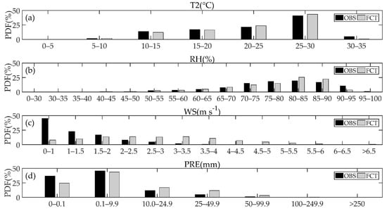
Figure 3.
The probability density function (PDF) of daily averaged values for T2 (a), RH (b), WS (c) and PRE (d). OBS is observed values and FCT is simulated values.
In order to test the extreme climate by a downscaling simulation, the simulated extreme weather indices were compared with the observed values, and the MB and percentage of MB between the simulated and observed values were calculated (Table 5). For an extreme temperature, the MB basically meets the criteria value of T2 in HR (<2.0 °C), indicating that WRF dynamical scaling at an extreme temperature is acceptable. The MB and its percentage error of DTR are 2.0 °C and 11.9%, respectively. The WRF model can well-reproduce the daily variation range in temperature in the PRD region. For five extreme temperatures, the MB of TNx is the smallest, while the MB of TNn is the largest. WRF can better reproduce an extreme high temperature than an extreme low temperature. This may be related to the following factors. Generally, a high temperature usually occurs in sunny weather, while a low temperature is usually accompanied by cold air and precipitation. The uncertainty of cloud and precipitation may result in temperature error. It is worth noting that simulated temperature extremes exhibit obvious cold deviation, especially for extremely low temperatures, and they are larger than the cold deviation of the average temperature (Table 5). Previous studies have proposed that this may be related to the lack of some physical processes, such as the urban canopy effect of anthropogenic heat [39]. Due to the obvious urbanization characteristics in the PRD region and the influence of the obvious urban heat island effect, the temperature at night is increased by anthropogenic heat. However, the influence of the urban canopy and anthropogenic heat ignored in this paper results in cold deviation of the simulated temperature. The smaller the temperature, the weaker the turbulent mixing, resulting in more obvious cold deviation for extremely low temperatures.
Table 5.
The comparison of extreme weather indices for simulation and observation data collected during 2013–2017 over Pearl River Delta.
For PRE, a relatively large error in extreme precipitation simulation can be detected. The percentage errors of R10 and R20 are 81.5% and 142.5%, respectively, which implies that WRF significantly overestimates extreme precipitation. The percentage error of R95t is only 22.9%. The observed average annual precipitation in the PRD region from 2013 to 2017 is 2003.0 mm, but the simulated average annual precipitation is 45.4% higher than the observed value. The SDIIs of observed and simulated values are 11.6 and 17.5 mm day−1, respectively. Previous studies also found the overestimation of extreme precipitation for WRF [40]. Overestimation of the shortwave radiation and relevant convective available potential energy in southeastern China may be one of the reasons for the precipitation overestimation [41]. Generally, the performance of extreme temperature and precipitation in the PRD region is comparable to previous studies [42].
3.2. The Performance in Different Seasons
Table 6 shows the statistical indices for simulated and observed daily average meteorological elements in different seasons. Overall, we can see that the WRF model has the best simulation effect on T2, followed by RH2, and a relatively large error for the wind and precipitation simulation.
Table 6.
Statistical indices for simulated and observed daily averaged T2, RH2, WS, WD, and PRE during different seasons.
For T2 and RH2, the STD differences in all seasons of the T2 and RH2 simulation and observation can be ignored, which indicates that the WRF simulation can better show the dispersion degree of temperature and humidity. Seasonally, the T2 simulation result slightly overestimates the observation value in spring, with the MB of 0.43 °C, and other seasons’ simulations underestimate the T2, but their numerical biases are small. This may be related to the complex spring rainfall period in PRD and it can be seen from Table 6 that the model has a poor simulation of spring precipitation, which may indirectly affect the model simulation result of T2. For the summer, it is also shown in Table 6 that the simulation result error in summer is relatively large for T2 and RH2, compared with other seasons, with R values of 0.74 and 0.77, respectively. Davis et al.’s (2002) studies indicate that this may be related to the systematic error of the cumulus parameterization scheme [43]. The PRD in summer is susceptible to the influence of the typhoon and tropical storm, and this kind of cumulus scale is generally small, while the energy spectrum gap between the scale and mesoscale of cumulus described in the scheme of cumulus convection parameterization used in the WRF model is larger than that of the real atmosphere, with larger errors, so it will have a certain influence on the simulation results. Furthermore, the particularly strong moisture transport of PRD in the summer is also one of the factors that caused the MB overestimation of RH2.
For wind, most of the correlation coefficients (except spring) meet R > 0.8, which indicates that the WRF model can accurately simulate the seasonal variation characteristics of the wind speed. In terms of individual seasons, the R and IA in spring and summer are lower than in autumn and winter, but the HR (RMSE) is higher (lower) than in autumn and winter. One of the reasons for this result may be that extreme weather frequently occurs in spring and summer, and the weather situation is unstable and wind frequency is higher when the number of samples is larger. In autumn and winter, the weather situation is stable, the wind frequency is lower, and the sample number is smaller than in spring and summer, which may cause certain random error, making the HR relatively poor. The results of Analysis of Variance (ANOVA) show that the simulation values of WRF are significantly overestimated all year. This is similar to previous studies [44]. There are many reasons for the simulation overestimation of WS. The YSU parameterization scheme selected in this study has a better simulation effect on WRF than other schemes, but it also leads to strong mixing of the simulated turbulence, which leads to overestimation of the surface wind speed in the model [45]. On the other hand, some studies have also proved that the surface wind speed of FNL data is 33% higher than the observed value, so the higher wind speed of FNL data as a driving field may also lead to the simulation overestimation of wind speed in the WRF model [19].
It can be seen from Table 6 that the WRF model can roughly simulate the seasonal characteristics of precipitation by comparing the observed values, and the simulated STD displays a large deviation from the observed values, which indicates that the WRF model overestimates the fluctuation range of precipitation. From the perspective of the season, the WRF model seriously overestimates the precipitation of the whole year, and the deviation of spring is large. This may be related to the fact that, in spring, the PRD is in the pre-flood season in southern China, and the subtropical high moves northward, making the cold and warm air flow converge in south China. This superimposes the influence of the low-altitude southwest jet over south China, resulting in the complexity of rainfall, which leads to the simulation deviation. In summer, although the simulation effect is relatively good, R and IA are 0.77 and 0.86, respectively, but MB also reaches 12.08 mm, which seriously overestimates the precipitation in summer. As mentioned in the above section, the PRD is very vulnerable to typhoons and tropical storms in the summer, and most of the summer is rainstorm and above. This also indirectly explains why the simulation effect in winter is relatively good, because there is less rainfall and a lower rainfall intensity in winter.
Based on the above research on the progress of the simulation value and observation value of the daily average variation of each meteorological element in the four seasons, the WRF model can preferably simulate the characteristics of various meteorological elements in different seasons. The simulation results of autumn and winter are the best, followed by spring, and in summer, the PRD is vulnerable to extreme weather, such as typhoons and tropical storms, so the simulation effect is relatively poor.
3.3. The Performance in Different Circulation Types
Table 7 shows the statistical indices for simulated and observed daily average meteorological elements in different circulation types.
Table 7.
Statistical indices for simulated and observed daily averaged T2, RH2, WS, WD, and PRE for different circulation types.
For T2 and RH2, the simulations of nine circulation types all meet the statistical benchmark (IA > 0.8) [34], and their MBs have small values, indicating that the WRF model could basically simulate the temperature and relative humidity characteristics of different circulation types. However, relative to other types of circulation, the simulation results under CT1, CT4, and CT7 are relatively poor. CT1 mainly appears in the spring and summer, during the pre-flood period in south China. The confrontation of warm and cold air flow in the pre-flood period leads to small-scale weather, such as cold fronts, shear lines, and so on, which easily leads to temperature fluctuation and a range of extreme precipitation. Previous studies show that the error of the WRF model for the simulation of this kind of weather system is relative large [46]. CT4 and CT7 mainly appear in the summer. The PRD is mainly affected by typhoons or tropical cyclones under CT4, and affected by weak low pressure under CT7. Generally, WRF dynamical downscaling has relatively poor performance under weather conversion (CT1) or cloudy and rainy weather (CT4 and CT7) due to the dynamic or physical process defects of the model itself [47]. The large error of FNL data in such weather also passes to downscaling simulations.
The WS simulation of WRF for different circulation types is more complicated. According to the MB in Table 7, WRF overestimates the wind speed of all circulation types, and the simulation values of all STDs are larger than the observed values, indicating that WRF overestimates the wind speed and fluctuation range under all circulation types. Previous studies also reported that WRF overestimates near-surface wind speed, which maybe relate to the error of physical parameterization schemes [16]. Another may be due to the high level of urbanization distribution in the PRD, but the urban canopy parameters are not considered in this paper, which makes the WRF model underestimate the friction weakening effect of the city on WS [45]. In different circulation types, WRF model can better reproduce the wind field variation characteristics under CT2, CT4, CT5, CT6, and CT9, with R exceeding 0.80. For CT2, CT5, and CT9, the isobar is relatively dense (Figure 2) which results in large pressure gradient and wind speed. The CT4 and CT6 are mainly controlled by typhoons or tropical cyclones, the wind speed is also large. In large background wind, mesoscale model can well reproduce time variation characteristics of wind speed (high R), while brings large RMSE and MB, and vice versa [48]. CT3 (CT7) is located at the rear of anticyclone (cyclone), and easy to produce small-scale motion which leading wind field to complex. CT1 and CT8 appears in spring, which is affected by the pre-flood period in south China, there are a lot of wind shear lines which cause the wind field more complex. Above of that make the simulation results of CT1 and CT8 are relatively poor. Generally, WRF model overestimates the WS in all circulation types. When the pressure gradient in the PRD is large (CT2, CT5, CT9) or controlled by typhoon (CT4, 6), the wind speed is relatively large, WRF can well reproduce time variation characteristics, but brings large absolute error. When PRD located at the rear of anticyclone (CT3), cyclone (CT7) or controlled by pre-flood period (CT1, CT8), the weather situation becomes complex, the performance of WRF is affected [47].
For PRE, when the circulation types are CT2, CT3, CT5, and CT9, the PRE simulation meets the statistical benchmark (IA > 0.6) [34]. CT2, CT5, and CT9 is control by high-pressure and CT3 locate at edge of high-pressure (Figure 2), and the deviation of MB is relatively small which indicates that the model can better simulate PRE under these types. For CT1, CT4, CT6, CT7, and CT8, their MB plus deviations are large, which indicates that the model seriously overestimates the PRE under there five circulation types. The PRD is affected by pre-flood season of south China (CT1 and CT8), controlled by typhoons or tropical cyclones (CT4 and CT6) or rear of weak depression (CT7), resulting in frequent severe convective weather, and increased extreme precipitation. WRF model has poor simulation on this kind of precipitation [37,47]. Above of those leads to the deviation of those circulation types simulation result. The simulated STD of the four circulation types displays a large deviation from the observed values, which indicates that the WRF model overestimates the fluctuation range of precipitation. Vuillaume and Hearth (2018) pointed out that there are variations of different circulation types, an optimized physical parameterization schemes maybe change with different weather types [49]. Overall, compared with other meteorological factors, the simulated precipitation are relatively poor for all circulation types, and there is a large deviation of MB when PRD affected by pre-flood period in south China (CT1 and CT8) or control by low-pressure (CT4, CT6, and CT7), but the deviation of MB when PRD is control by high-pressure (CT2, CT3, CT5, and CT9) is relatively small, and the effect of R and IA is relatively good.
According to the movement of the subtropical anticyclone, the evolution of the weather situation in the PRD can be divided into four steps. In spring, the cold southward air converges with the subtropical anticyclone in the PRD. The cold and warm current are equally strong, forming strong wind easily. This circulation leads to temperature reduction and heavy rain, affecting the simulation effect of WRF (CT1 and CT8). At the end of spring, the subtropical anticyclone rises to the north, the PRD main at the rear of weak high (CT3) or weak depression (CT7). WRF can well reproduce the meteorological fields (T2, RH2, PRE) in these weather situations. However, for wind field, the northward movement of the subtropical high produces a lot of wind shear lines, which makes the result of WS simulation more complicated. In summer, the South China Sea monsoon begins to break out. The monsoon’s northward movement is affected by land uplift and other factors, which brings a large continuous rainfall in the PRD. In this period, the PRD is affected typhoons or tropical cyclones easily, and WRF is prone to producing a large error due to uncertainty of cloud microphysical simulation (CT4 and CT6). In autumn and winter, the subtropical anticyclone begins to move southward. The PRD is mainly controlled by high pressure (CT2, CT5, and CT9), the weather situation tends to be stable. WRF can well reproduce stable weather.
Generally, when the PRD is located at the center or rear of the high pressure, the atmospheric junction is relatively stable, and the WRF simulation effect is better. When the PRD is controlled by low pressure or affected by typhoons and other factors, the pressure gradient is large, and the atmospheric junction is unstable, so the simulation effect is relatively poor.
4. Conclusions
In this study, NCEP FNL operational global analysis data were used as the driving field of the regional climate model WRF to carry out numerical experiments of dynamic downscaling in the Pearl River Delta region during the five years of 2013–2017. The simulation results and observation data were compared and analyzed, and the simulation ability of the WRF model for the regional climate was evaluated. The main conclusions are as follows:
1. Overall, the WRF model can very well simulate the change characteristics of 2-m temperature and 2-m relatively humidity, with HR (hit rate) values of 92.66% and 93.98%, respectively. The results of variance analysis show that the 10-m wind speed simulated by the WRF model was significantly overestimated. The precipitation simulation is relatively poor, WRF overestimates the annual precipitation, and it can be seen from the statistical indicators that WRF has a good simulation effect for light rain and below, while the simulation for moderate rain exhibits a large deviation.
2. For extreme weather, the WRF model can well-reproduce the characteristics of temperature variation. For five extreme temperature indices, the MB (Mean Bias) of TNX (monthly maximum value of daily minimum temperature) is smallest, while the TNn (monthly minimum value of daily minimum temperature) is the largest, which indicate WRF model can better reproduce extreme high temperature than extreme low temperature. The result of precipitation simulation is relatively poor and WRF seriously overestimates the extreme rainfall.
3. The simulation performance of the WRF model has obvious seasonal differences. Overall, the WRF model produces the best simulation results in autumn and winter, followed by spring, while the summer results are relatively poor. The simulation of different meteorological factors shows that the WRF model can better reproduce the variation characteristics of 2-m temperature and 2-m relatively humidity in different seasons. For 10-m wind speed and precipitation, the WRF model overestimates the wind speed and rainfall in each season. The autumn and winter have a relatively good simulation effect, which is due to the stable weather pattern. However, in spring, WRF can well-reproduce the characteristics of 2-m temperature and 2-m relatively humidity, for 10-m wind and precipitation, the Pearl River Delta is affected by the flood season in southern China, the result of simulation is relatively poor. In summer, due to the influence of extreme weather, the deviation of all meteorological factor simulation is large.
4. The circulation type is an important parameter of downscaling assessment. When the Pearl River Delta region is located at the center or rear of the high pressure, the WRF simulation effect is better. When the Pearl River Delta region is under the control of low pressure or extreme weather, the atmospheric pressure gradient is large, and the atmospheric junction is unstable, so the simulation effect is relatively poor.
In general, the dynamical downscaling method can certain extent improve the resolution and accuracy of meteorological elements in the Pearl River Delta region. This paper analyzes the influence of different extreme weather and different seasons on dynamical downscaling. At the same time, there is less researches focusing on the impact of weather classification on dynamic downscaling in the Pearl River Delta region, which is studied in this paper. Limited by computing resources, this paper only studies the impact of meteorological conditions, but lacks the research on the impact of model errors on dynamical downscaling. In the future, it is still necessary to study the impact of other factors on dynamical downscaling, such as the influence of different reanalysis data and using more detailed parameterization scheme.
Author Contributions
Writing—original draft preparation, C.Z. and J.H.; writing—review and editing, C.Z. and J.H.; visualization, Y.L. and C.Z.; supervision, J.H., X.L., H.C. and S.G.; funding acquisition, J.H. and S.G. All authors have read and agreed to the published version of the manuscript.
Funding
This work was supported by the National Natural Science Foundation of China (No. 41975131, 41705080), the CAMS Basis Research (No. 2017Y001, 2019Z009), Key Laboratory of South China Sea Meteorological Disaster Prevention and Mitigation of Hainan Province fund (SCSF201802), and the CMA Innovation Team for Haze-fog Observation and Forecasts.
Institutional Review Board Statement
Not applicable.
Informed Consent Statement
Not applicable.
Data Availability Statement
The data presented in this study are available on request from the corresponding author. The data are not publicly available due to the size of the simulation archive.
Conflicts of Interest
The authors declare no conflict of interest.
References
- Feng, K. Characteristics and Comparison of Different Downscaling Methods in Global Climate Model. Meteorol. Environ. Res. 2020, 11, 44–48. [Google Scholar] [CrossRef]
- Wang, J.; Zhi, X.F.; Chen, Y.W. Probabilistic Multimodel Ensemble Prediction of Decadal Variability of East Asian Surface Air Temperature Based on IPCC-AR5 Near-term Climate Simulations. Adv. Atmos. Sci. 2013, 30, 1129–1142. [Google Scholar] [CrossRef]
- Wilby, R.L.; Dawson, C.W.; Barrow, E.M. SDSM-A decision support tool for the assessment of regional climate change impacts. Environ. Model. Softw. 2002, 17, 145–157. [Google Scholar] [CrossRef]
- Liu, Y.; Fan, K.; Chen, L.J.; Ren, H.L. An operational statistical downscaling prediction model of the winter monthly temperature over China based on a multi-model ensemble. Atmos. Res. 2021, 249, 105262. [Google Scholar] [CrossRef]
- Kumar, B.; Chattopadhyay, R.; Singh, M.; Chaudhari, N.; Kodari, K.; Barve, A. Deep learning–based downscaling of summer monsoon rainfall data over Indian region. Theor. Appl. Climatol. 2021, 143, 1–12. [Google Scholar] [CrossRef]
- Pan, X.D.; Li, X.; Shi, X.K.; Han, J.N.; Luo, L.H.; Wang, L.X. Dynamic downscaling of near-surface air temperature at the basin scale using WRF-a case study in the Heihe River Basin, China. Front. Earth Sci. 2012, 6, 314–323. [Google Scholar] [CrossRef]
- Tong, C.H.; Yim, S.H.; Rothenberg, D.; Wang, C.; Lin, C.Y.; Chen, Y.D.; Lau, N.C. Assessing the impacts of seasonal and vertical atmospheric conditions on air quality over the Pearl River Delta region. Atmos. Environ. 2018, 180, 69–78. [Google Scholar] [CrossRef]
- You, C.; Fung, C.H. Characteristics of Sea-breeze Circulation in the Pearl River Delta Region and Its Dynamical Diagnosis. J. Appl. Meteorol. Climatol. 2019, 58, 741–755. [Google Scholar] [CrossRef]
- Mooney, P.A.; Mulligan, F.J.; Fealy, R. Evaluation of the sensitivity of the weather research and forecasting model to parameterization schemes for regional climates of Europe over the period 1990-95. J. Clim. 2013, 26, 1002–1017. [Google Scholar] [CrossRef]
- Otte, T.L.; Nolte, C.G.; Otte, M.J.; Bowden, J.H. Does Nudging Squelch the Extremes in Regional Climate Modeling? J. Clim. 2012, 25, 7046–7066. [Google Scholar] [CrossRef]
- Wang, B.; Yang, H.W. Hydrological issues in lateral boundary conditions for regional climate modeling: Simulation of east asian summer monsoon in 1998. Clim. Dyn. 2008, 31, 477–490. [Google Scholar] [CrossRef]
- Guo, J.; Huang, G.; Wang, X.; Li, Y.; Lin, Q. Investigating future precipitation changes over China through a high-resolution regional climate model ensemble. Earth Future 2017, 5, 285–303. [Google Scholar] [CrossRef]
- Qiu, Y.; Hu, Q.; Zhang, C. WRF simulation and downscaling of local climate in Central Asia. Int. J. Climatol. 2017, 37, 513–528. [Google Scholar] [CrossRef]
- Gao, X.J.; Zhao, Z.C.; Ding, Y.H.; Huang, R.H.; Giorgi, F. Climate change due to greenhouse effects in China as simulated by a regional climate model. Acta Meteorol. Sin. 2003, 17, 417–427. [Google Scholar] [CrossRef]
- Jiménez, P.A.; González-Rouco, J.F.; García-Bustamante, E. Surface Wind Regionalization over Complex Terrain: Evaluation and Analysis of a High-Resolution WRF Simulation. J. Appl. Meteorol. Climatol. 2008, 49, 268–287. [Google Scholar] [CrossRef]
- He, J.J.; Yu, Y.; Liu, N.; Zhao, S.P. Impact of land surface information on WRFs performance in complex terrain area. Chin. J. Atmos. Sci. 2014, 38, 484–498. [Google Scholar] [CrossRef]
- Skamarock, W.C.; Klemp, J.B.; Dudhia, J.; Gill, D.O.; Powers, J.G. A Description of the Advanced Research WRF Version 3. Univ. Corp. Atmos. Res. 2008. [Google Scholar] [CrossRef]
- Pérez, J.C.; Díaz, J.P.; González, A.; Expósito, J.; Taima, D. Evaluation of WRF Parameterizations for Dynamical Downscaling in the Canary Islands. J. Clim. 2013, 27, 5611–5631. [Google Scholar] [CrossRef]
- Yu, L.J.; Yin, C.M.; Lin, Y.C.; He, J.J. Study of Dynamical Downscaling on Near Surface Wind Speed over China. J. Arid Meteorol. 2017, 35, 23–28. [Google Scholar] [CrossRef]
- Lopes, D.; Ferreira, J.; Hoi, K.I.; Miranda, A.I.; Yuen, K.V.; Mok, K.M. Weather research and forecasting model simulations over the Pearl River Delta Region. Air Qual. Atmos. Health 2019, 12, 115–125. [Google Scholar] [CrossRef]
- Wen, J.; Chen, J.; Lin, W.; Jiang, B.; Xu, S.; Lan, J. Impacts of Anthropogenic Heat Flux and Urban Land-Use Change on Frontal Rainfall near Coastal Regions: A Case Study of a Rainstorm over the Pearl River Delta, South China. J. Appl. Meteorol. Climatol. 2020, 59, 363–379. [Google Scholar] [CrossRef]
- Wang, E.T.; Sun, H.J.; Jian, Q. A Quick Report on a Dynamical Downscaling Simulation over China Using the Nested Model. Atmos. Ocean. Sci. Lett. 2010, 3, 325–329. [Google Scholar] [CrossRef]
- Zhang, B.H.; Liu, S.H.; Liu, H.P.; Ma, Y.J. The effect of MYJ and YSU schemes on the simulation of boundary layer meteorological factors of WRF. Chin. J. Geophys 2012, 55, 2239–2248. [Google Scholar] [CrossRef]
- Bowden, J.H.; Nolte, C.G.; Otte, T.L. Simulating the impact of the large-scale circulation on the 2-m temperature and precipitation climatology. Clim. Dyn. 2013, 40, 1903–1920. [Google Scholar] [CrossRef]
- Stauffer, D.R.; Seaman, N.L. Multiscale Four-Dimensional Data Assimilation. J. Appl. Meteorol. 1994, 33, 416–434. [Google Scholar] [CrossRef]
- Kim, Y.H.; Min, S.K.; Zhang, X.; Zwiers, F.; Alexander, L.V.; Donat, M.G.; Tung, Y.S. Attribution of extreme temperature changes during 1951–2010. Clim. Dyn. 2016, 46, 1769–1782. [Google Scholar] [CrossRef]
- Xie, P.P.; Yatagai, A.; Chen, M.Y.; Hayasaka, T.; Fukushima, Y.; Liu, C.M.; Yang, S. A Gauge-Based Analysis of Daily Precipitation over East Asia. J. Hydrometeor. 2007, 8, 607. [Google Scholar] [CrossRef]
- Jiménez, P.A.; Dudhia, J. Improving the Representation of Resolved and Unresolved Topographic Effects on Surface Wind in the WRF Model. J. Appl. Meteorol. Climatol. 2012, 51, 300–316. [Google Scholar] [CrossRef]
- Soares, P.M.M.; Cardoso, R.M.; Miranda, P.M.A.; de Medeiros, J.; Belo-Pereira, M.; Espirito-Santo, F. WRF high resolution dynamical downscaling of ERA-Interim for Portugal. Clim. Dyn. 2012, 39, 2497–2522. [Google Scholar] [CrossRef]
- Perkins, S.E.; Pitman, J.A.; Holbrook, N.J.; Mcaneney, J. Evaluation of the AR4 Climate Models’ Simulated Daily Maximum Temperature, Minimum Temperature, and Precipitation over Australia Using Probability Density Functions. J. Clim. 2007, 20, 4356–4376. [Google Scholar] [CrossRef]
- Conner, M.; Petty, G. Validation and Intercomparison of SSM/I Rain-Rate Retrieval Methods over the Continental United States. J. Appl. Meteorol. 1998, 37, 679–700. [Google Scholar] [CrossRef]
- Willmott, C.J.; Ackleson, S.G.; Davis, R.E.; Feddema, J.J.; Klink, K.M.; Legates, D.R.; O’Donnell, J.; Rowe, C.M. Statistics for the evaluation and comparison of models. J. Geophys. Res. Ocean. 1985, 90, 8995–9005. [Google Scholar] [CrossRef]
- He, J.; Gong, S.; Zhou, C.; Lu, S.; Wu, L.; Chen, Y.; Yu, Y.; Zhao, S.; Yu, L.; Yin, C. Analyses of winter circulation types and their impacts on haze pollution in Beijing. Atmos. Environ. 2018, 192, 94–103. [Google Scholar] [CrossRef]
- Porras, I.; Arasa, R.; Ángeles, M.; Jésica, G.; Bernat, P. Defining a Standard Methodology to Obtain Optimum WRF Configuration for Operational Forecast: Application over the Port of Huelva (Southern Spain). Atmos. Clim. Sci. 2016, 6, 329–350. [Google Scholar] [CrossRef]
- Jiang, P.; Liu, X.R.; Zhu, H.N.; Zhu, Y.; Zeng, W.X. Idealized Numerical Simulation of Local Mountain-Valley Winds over Complex Topography. Plateau Meteorol. 2019, 38, 1272–1282. [Google Scholar] [CrossRef]
- Shimada, S.; Ohsawa, T.; Chikaoka, S.; Kozai, K. Accuracy of the Wind Speed Profile in the Lower PBL as Simulated by the WRF Model. Entific Online Lett. Atmos. SOLA 2011, 7, 109–112. [Google Scholar] [CrossRef]
- Mei, Q.; Zhi, X.F.; Wang, J. Verification and consensus experiments of rainstorm forecasting using different cloud parameterization schemes in WRF model. Trans. Atmos. Sci. 2018, 41, 731–742. [Google Scholar] [CrossRef]
- Huang, D.L.; Gao, S.B. Impact of different reanalysis data on WRF dynamical downscaling over China. Atmos. Res. 2018, 200, 25–35. [Google Scholar] [CrossRef]
- Zhang, D.L.; Shou, Y.X.; Dickerson, R.R. Upstream urbanization exacerbates urban heat island effects. Geophys. Res. Lett. 2009, 36, 88–113. [Google Scholar] [CrossRef]
- Gao, Y.; Xue, Y.; Peng, W.; Kang, H.-S. Assessment of dynamic downscaling of the extreme rainfall over East Asia using a regional climate model. Adv. Atmos. Sci. 2011, 28, 1077–1098. [Google Scholar] [CrossRef]
- Zhao, S.P.; Yu, Y.; Qin, D.H.; Yin, D.Y.; He, J.J. Assessment of long-term and large-scale even-odd license plate controlled plan effects on urban air quality and its implication. Atmos. Environ. 2017, 170, 82–95. [Google Scholar] [CrossRef]
- Zhang, J.; Wu, L.; Dong, W. Land-atmosphere coupling and summer climate variability over East Asia. J. Geophys. Res. Atmos. 2011, 116, D05117. [Google Scholar] [CrossRef]
- Davis, C.; Bosart, L.F. Numerical Simulations of the Genesis of Hurricane Diana (1984). Part II: Sensitivity of Track and Intensity Prediction. Mon. Weather. Rev. 2002, 130, 1100–1124. [Google Scholar] [CrossRef]
- Zhao, C.L.; Zhang, T.J.; Wang, W.; Liu, Y.P.; Zeng, D.W.; Li, Y.H. Impacts of Land-use Data on the Simulation of 10 m Wind Speed in Northwest China. J. Arid Meteorol. 2018, 36, 397–404. [Google Scholar] [CrossRef]
- Zhang, J.P.; Zhu, T.; Zhang, Q.H.; Li, C.C.; Shu, H.L.; Ying, Y.; Dai, Z.P.; Wang, X.; Liu, X.Y.; Liang, A.M. The impact of circulation patterns on regional transport pathways and air quality over Beijing and its surroundings. Atmos. Chem. Phys. 2012, 11, 33465–33509. [Google Scholar] [CrossRef]
- Hon, K.K. Tropical cyclone track prediction using a large-area WRF model at the Hong Kong Observatory. Trop. Cyclone Res. Rev. 2020, 9, 64–74. [Google Scholar] [CrossRef]
- Ojrzyska, H.; Kryza, M.; Waaszek, K.; Szymanowski, M.; Werner, M.; Dore, A.J. High-Resolution Dynamical Downscaling of ERA-Interim Using the WRF Regional Climate Model for the Area of Poland. Part 2: Model Performance with Respect to Automatically Derived Circulation Types. Pure Appl. Geophys. 2017, 174, 527–550. [Google Scholar] [CrossRef]
- Miao, S.; Chen, F.; Lemone, M.A.; Tewari, M.; Wang, Y. An Observational and Modeling Study of Characteristics of Urban Heat Island and Boundary Layer Structures in Beijing. J. Appl. Meteorol. Climatol. 2009, 48, 484–501. [Google Scholar] [CrossRef]
- Vuillaume, J.F.; Hearth, S. Dynamic downscaling based on weather types classification: An application to extreme rainfall in south-east Japan. J. Flood Risk Manag. 2018, 11, e12340. [Google Scholar] [CrossRef]
Publisher’s Note: MDPI stays neutral with regard to jurisdictional claims in published maps and institutional affiliations. |
© 2021 by the authors. Licensee MDPI, Basel, Switzerland. This article is an open access article distributed under the terms and conditions of the Creative Commons Attribution (CC BY) license (http://creativecommons.org/licenses/by/4.0/).