
Gap Filling and Quality Control Applied to Meteorological Variables Measured in the Northeast Region of Brazil

 , ,
, ,  ,
,  , and
, and 
Abstract
1. Introduction
2. Materials and Methods
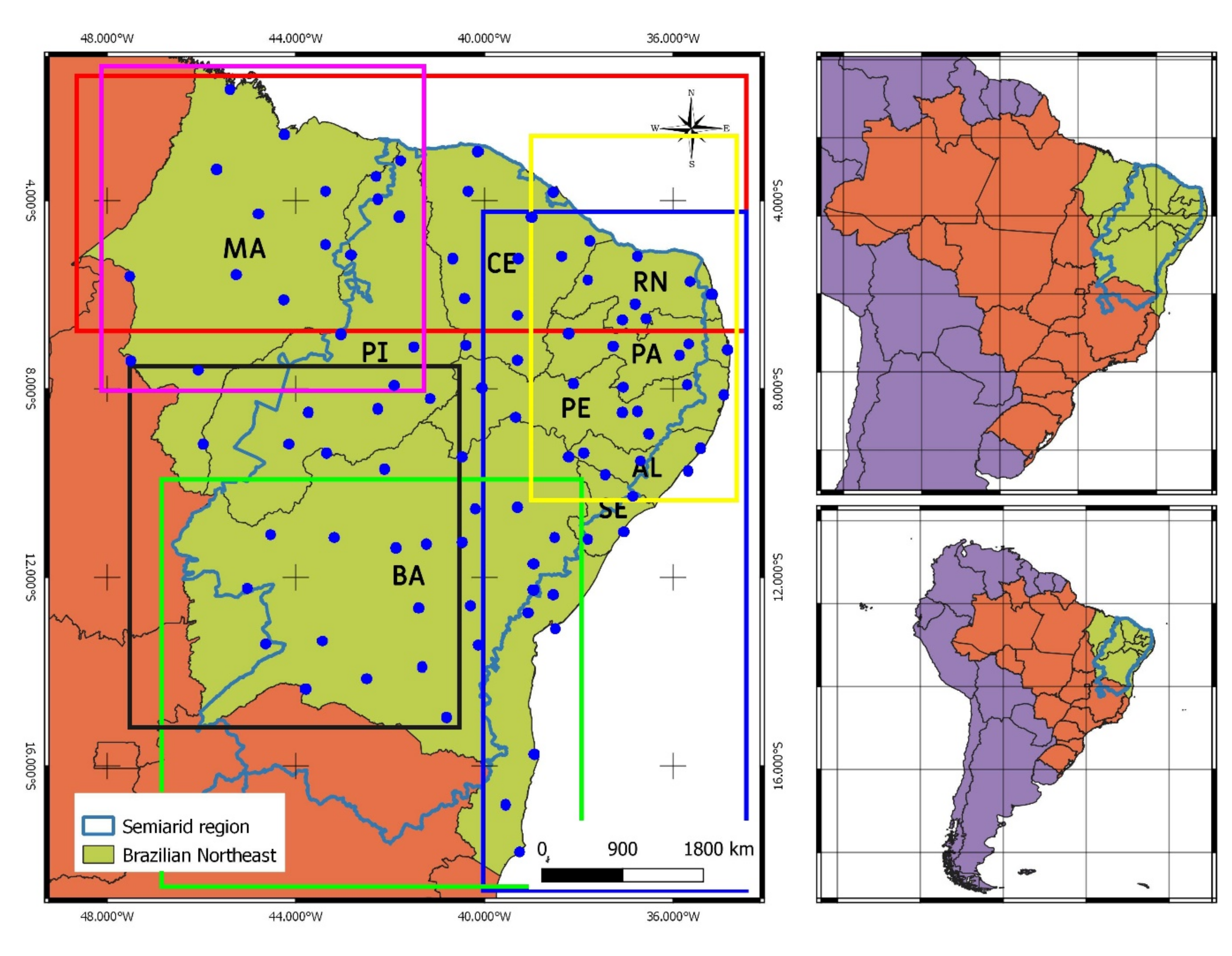
2.1. Area of Study and Data
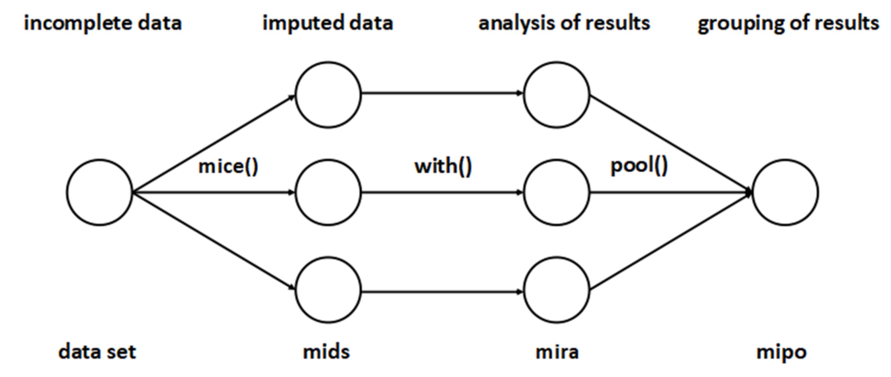
2.2. Filling in Missing Data
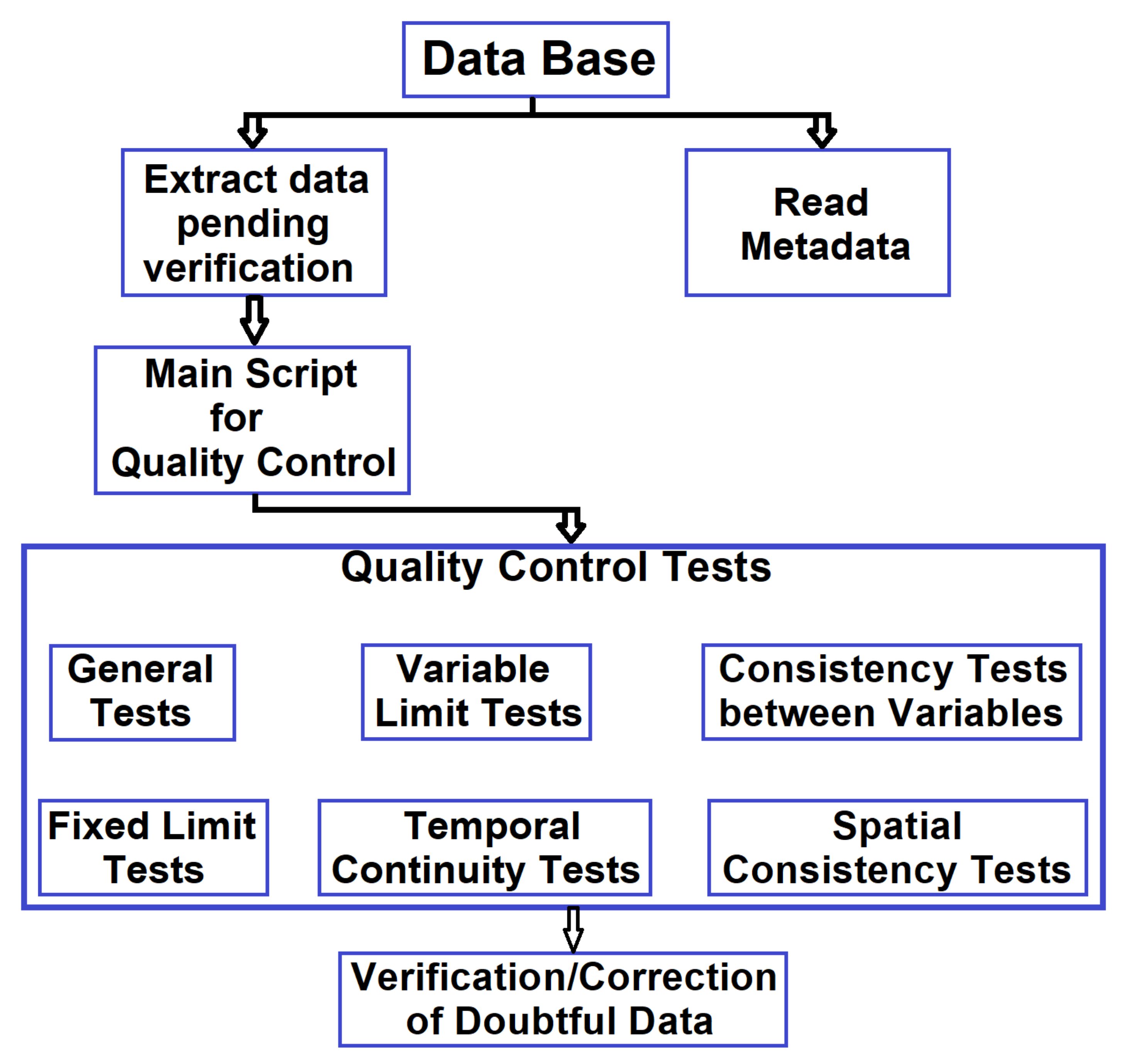
2.3. QCS
- Internal consistency tests express the physical relationships among different climatological elements. In some cases, they are logical tests based on the following premise: if a certain element exists in a given interval, another must also be contained in another interval [52].
- Temporal consistency tests are based on the persistence over time of climatological elements. Certain selected change thresholds depend on the variable in question, the period of the year and the climatic region to which the elements of the time series belong [53].
- Spatial consistency tests explore the smooth spatial variation of climatological variables. Generally, this type of test involves the estimation of a certain element based on neighbouring observations in the same climatic region [54]. The accepted limit of differences will depend on the type of variable, the climatic region and the distance between the seasons. Therefore, the effectiveness of this type of test will depend on the availability of neighbouring stations [55].
3. Results and Discussion
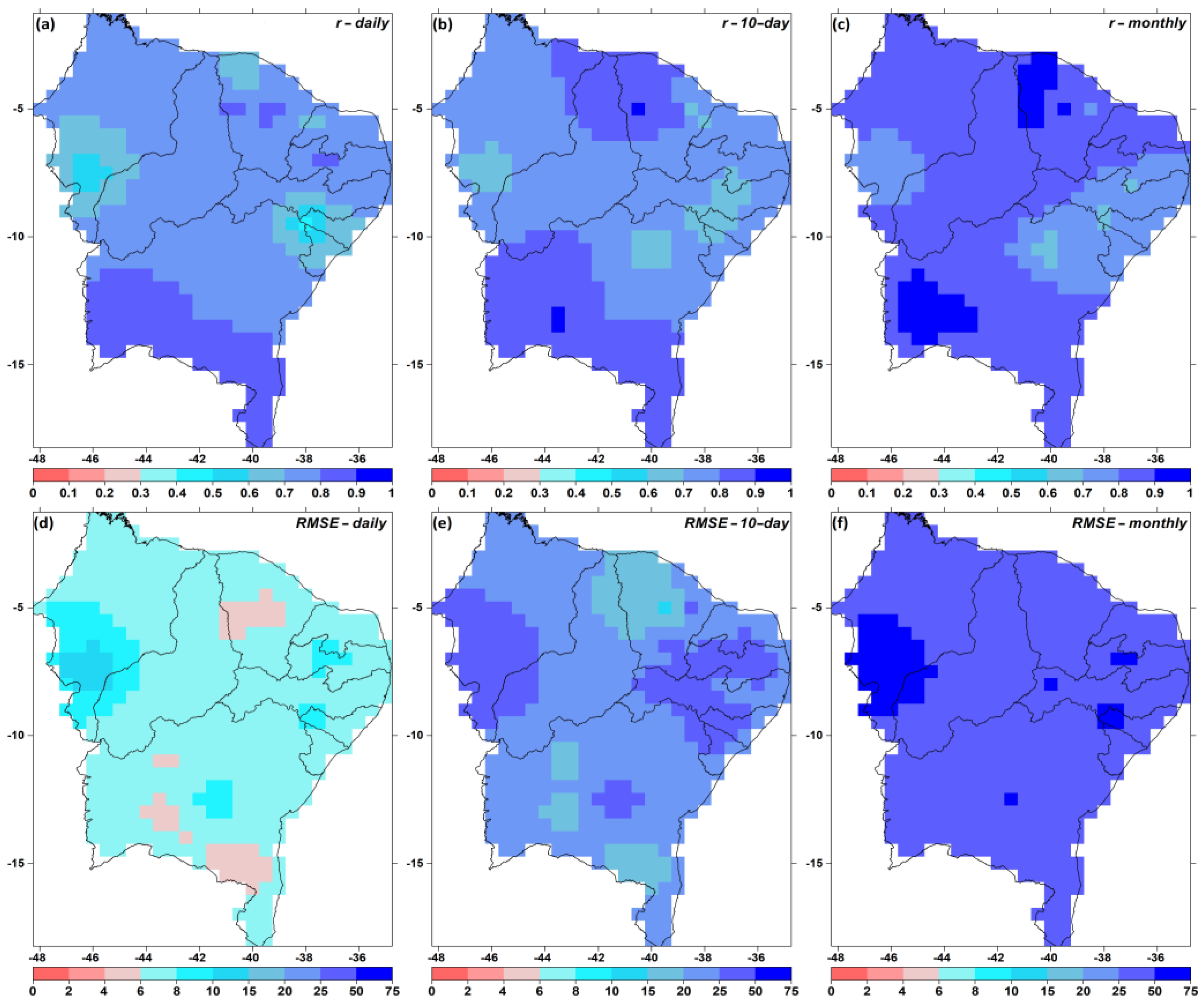
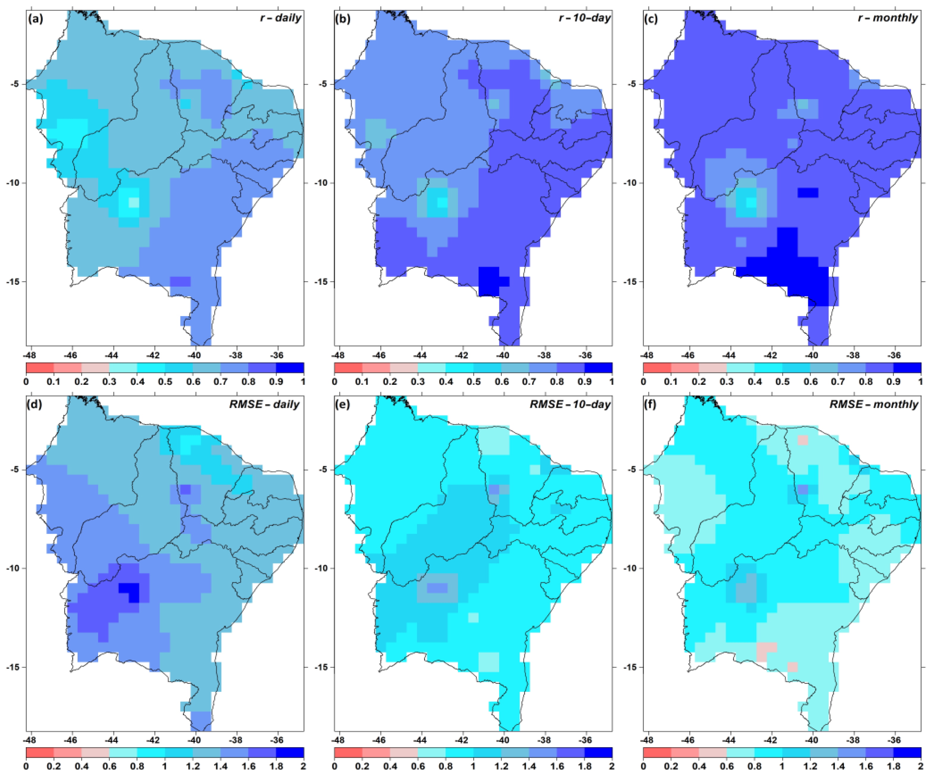
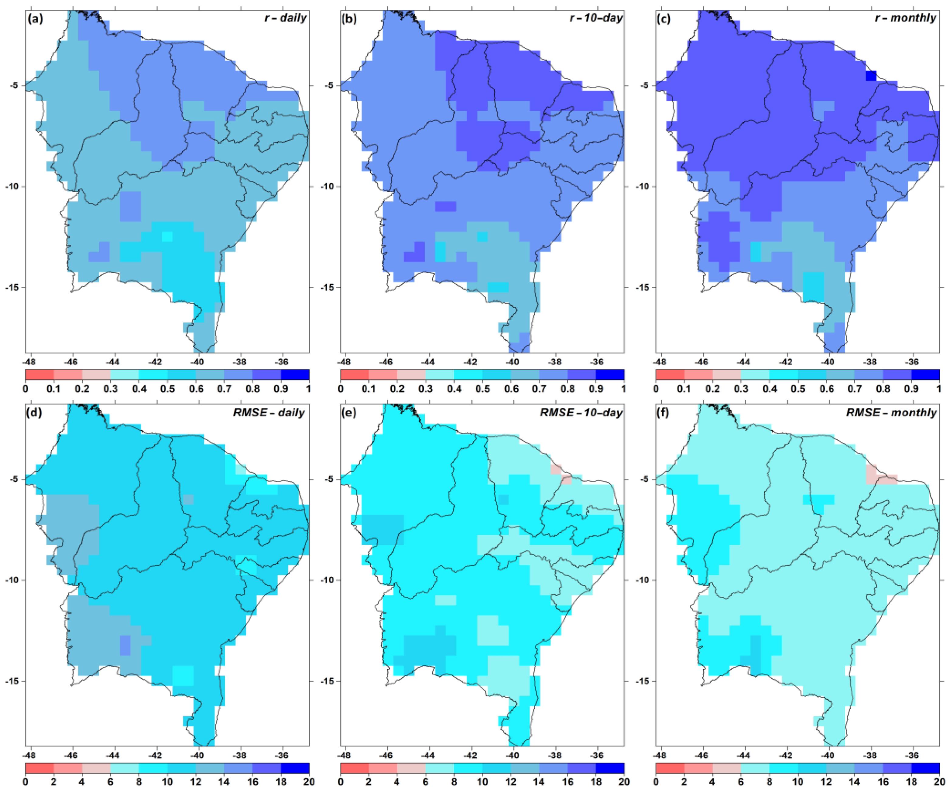
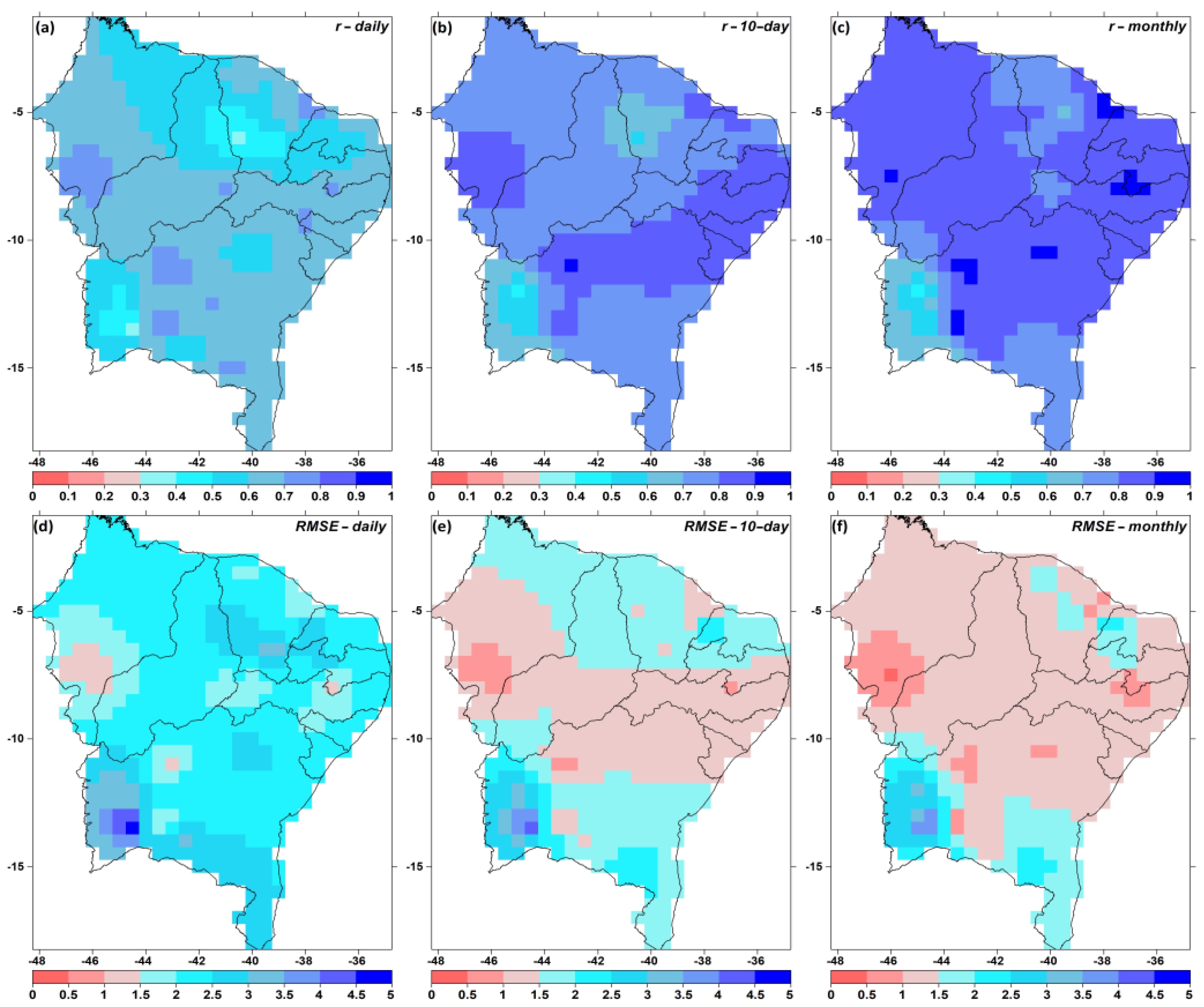
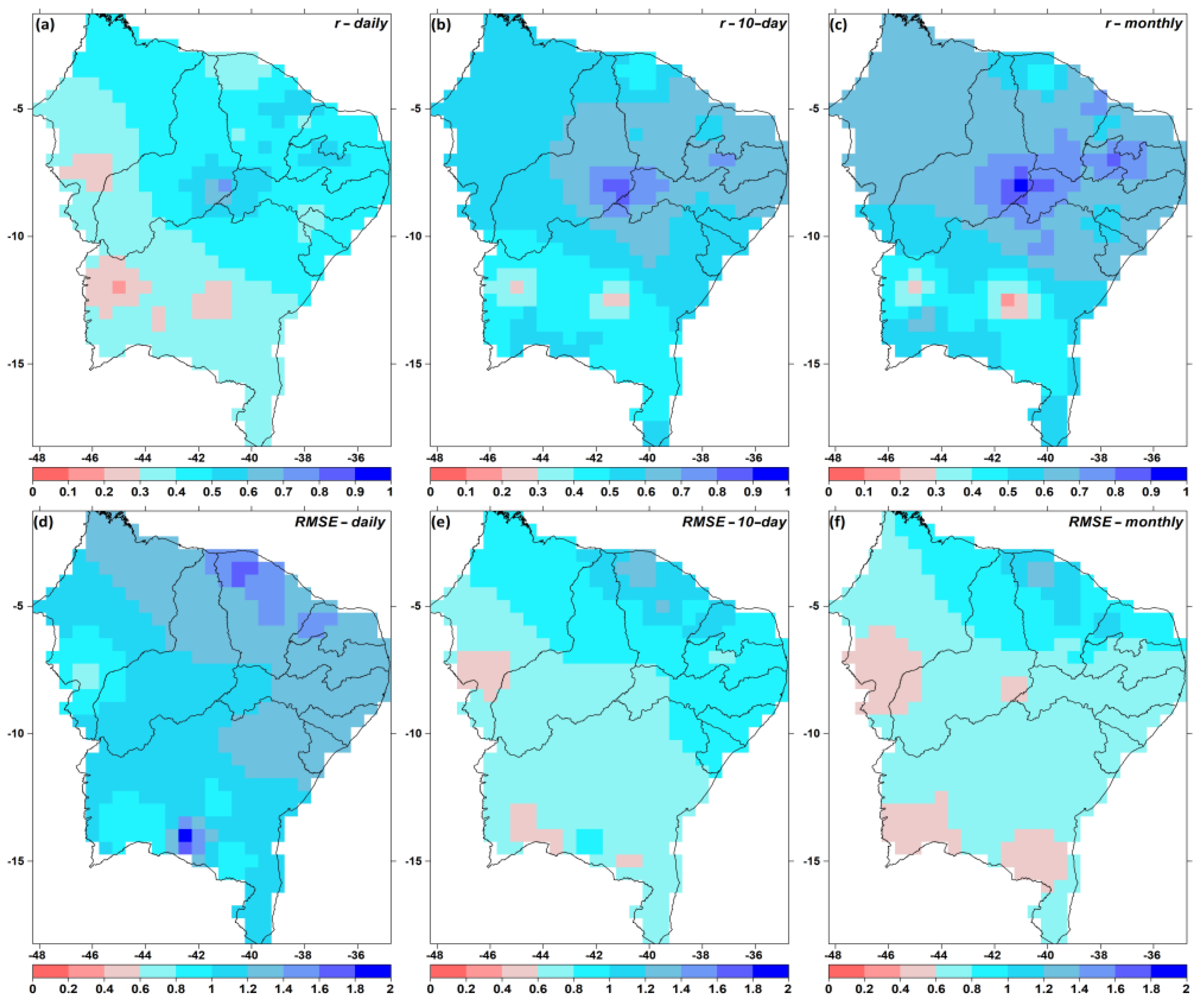
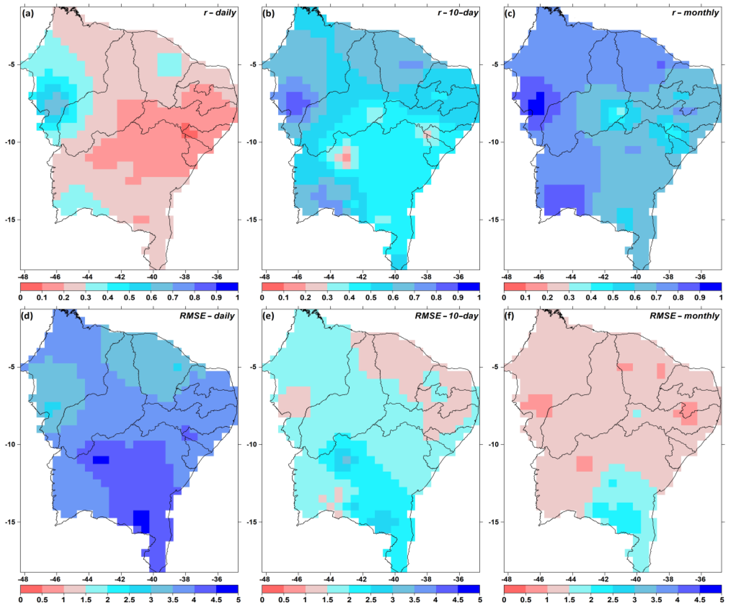
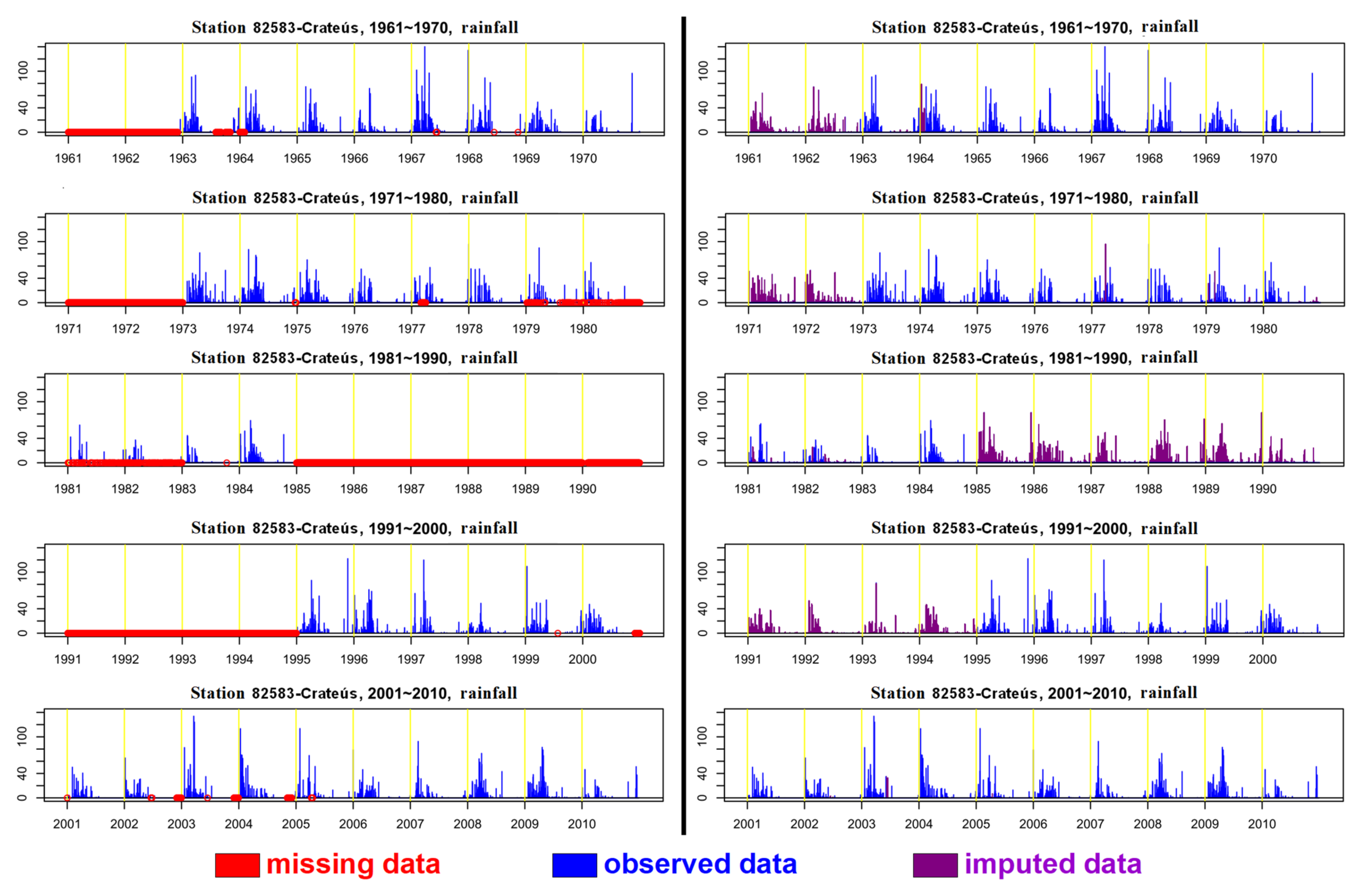
3.1. Gap Filling
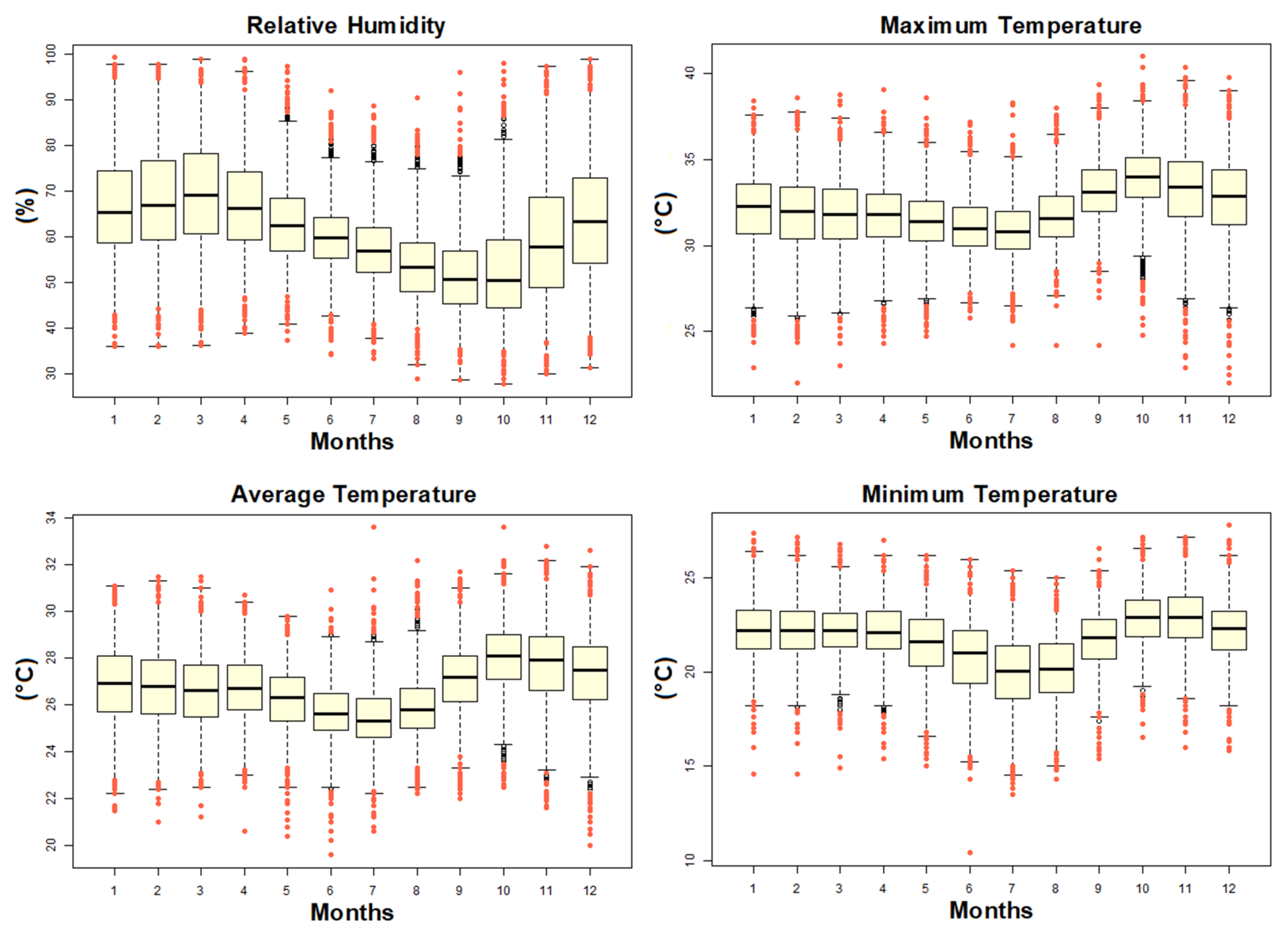
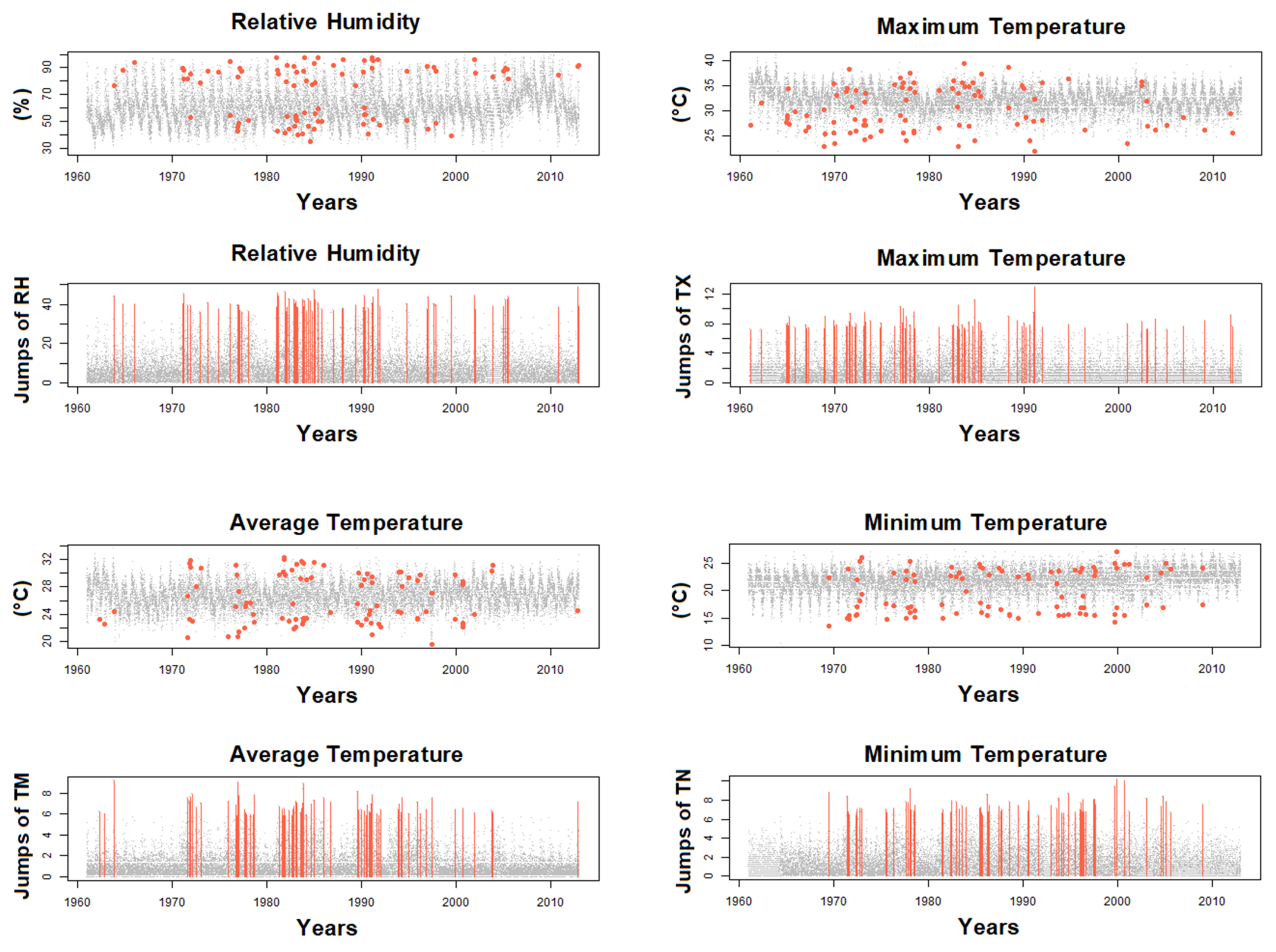
3.2. QCS
4. Conclusions
Author Contributions
Funding
Institutional Review Board Statement
Informed Consent Statement
Data Availability Statement
Acknowledgments
Conflicts of Interest
References
- Saurral, R.I.; Camilloni, I.A.; Barros, V.R. Low-frequency variability and trends in centennial precipitation stations in southern South America. Int. J. Climatol. 2016, 37, 1774–1793. [Google Scholar] [CrossRef]
- Carvalho, L.M.V. Assessing precipitation trends in the Americas with historical data: A review. WIREs Clim. Chang. 2020, 11, e627. [Google Scholar] [CrossRef]
- Sheffield, J.; Goteti, G.; Wood, E.F. Development of a 50-Year High-Resolution Global Dataset of Meteorological Forcings for Land Surface Modeling. J. Clim. 2006, 19, 3088–3111. [Google Scholar] [CrossRef]
- Costa, R.L.; de Mello Baptista, G.M.; Barros Gomes, H.; dos Santos Silva, F.D.; da Rocha Júnior, R.L.; Nedel, A.S. Analysis of future climate scenarios for northeastern Brazil and implications for human thermal comfort. An. Da Acad. Bras. De Ciências 2021, 93, e20190651. [Google Scholar] [CrossRef]
- Costa, R.L.; de Mello Baptista, G.M.; Barros Gomes, H.; dos Santos Silva, F.D.; da Rocha Júnior, R.L.; de Araújo Salvador, M.; Herdies, D.L. Analysis of climate extremes indices over northeast Brazil from 1961 to 2014. Weather Clim. Extrem. 2020, 28, 100254. [Google Scholar] [CrossRef]
- Liebmann, B.; Allured, D. Daily precipitation grids for South America. Bull. Am. Meteorol. Soc. 2005, 86, 1567–1570. [Google Scholar] [CrossRef]
- New, M.; Hulme, M.; Jones, P. Representing twentieth-century space–time climate variability. Part II: Development of 1901–96 monthly grids of terrestrial surface climate. J. Clim. 2000, 13, 2217–2238. [Google Scholar] [CrossRef]
- Silva, V.B.S.; Kousky, V.E.; Shi, W.; Higgins, R.W. An improved gridded historical daily precipitation analysis for Brazil. J. Hydrometeorol. 2007, 8, 847–861. [Google Scholar] [CrossRef]
- Xavier, A.C.; King, C.W.; Scanlon, B.R. Daily gridded meteorological variables in Brazil (1980–2013). Int. J. Climatol. 2016, 36, 2644–2659. [Google Scholar] [CrossRef]
- Xie, P.; Arkin, P.A. Global precipitation: A 17-year monthly analysis based on gauge observations, satellite estimates, and numerical model outputs. Bull. Am. Meteorol. Soc. 1997, 78, 2539–2558. [Google Scholar] [CrossRef]
- Huffman, G.J.; Adler, R.F.; Morrissey, M.M.; Bolvin, D.T.; Curtis, S.; Joyce, R.; McGavock, B.; Susskind, J. Global precipitation at one-degree daily resolution from multisatellite observations. J. Hydrometeorol. 2001, 2, 36–50. [Google Scholar] [CrossRef]
- Adler, R.F.; Huffman, G.J.; Chang, A.; Ferraro, R.; Xie, P.P.; Janowiak, J.; Rudolf, B.; Schneider, U.; Curtis, S.; Bolvin, D.; et al. The version-2 global precipitation climatology project (GPCP) monthly precipitation analysis (1979–present). J. Hydrometeorol. 2003, 4, 1147–1167. [Google Scholar] [CrossRef]
- Joyce, R.J.; Janowiak, J.E.; Arkin, P.A.; Xie, P. CMORPH: A method that produces global precipitation estimates from passive microwave and infrared data at high spatial and temporal resolution. J. Hydrometeorol. 2004, 5, 487–503. [Google Scholar] [CrossRef]
- Levizzani, V.; Bauer, P.; Turk, F.J. Measuring Precipitation from Space: Eurainsat and the Future; Springer Science & Business Media: Dordrecht, The Netherlands, 2007; Volume 28. [Google Scholar]
- Becker, A.; Finger, P.; Meyer-Christoffer, A.; Rudolf, B.; Schamm, K.; Schneider, U.; Ziese, M. A description of the global land-surface precipitation data products of the Global Precipitation Climatology Centre with sample applications including centennial (trend) analysis from 1901–present. Earth Syst. Sci. Data 2013, 5, 71–99. [Google Scholar] [CrossRef]
- Funk, C.; Peterson, P.; Landsfeld, M.; Pedreros, D.; Verdin, J.; Shukla, S.; Husak, G.; Rowland, J.; Harrison, L.; Hoell, A.; et al. The climate hazards infrared precipitation with stations: A new environmental record for monitoring extremes. Sci. Data 2015, 2, 150066. [Google Scholar] [CrossRef]
- Tapiador, F.J. Measuring Precipitation from Space. In Remote Sensing of Aerosols, Clouds, and Precipitation; Islam, T., Hu, Y., Kokhanovsky, A., Wang, J., Eds.; Elsevier: New York, NY, USA, 2018; pp. 211–221. [Google Scholar]
- Camargo, M.B.P.; Hubbard, K.G. Spatial and temporal variability of daily weather variables in sub-humid and semi-arid areas of the U.S. High Plains. Agric. For. Meteorol. 1999, 93, 141–148. [Google Scholar] [CrossRef]
- WMO. Guidelines on Climate Observation Networks and Systems; WMO Technical Document; WMO: Geneva, Switzerland, 2003. [Google Scholar]
- Guttman, N.V.; Quayle, R.G. A review of cooperative temperature data validation. J. Atmos. Ocean. Technol. 1990, 7, 334–339. [Google Scholar] [CrossRef]
- Meek, D.W.; Hatfield, J.L. Data quality checking for single station meteorological databases. Agric. For. Meteorol. 1994, 69, 85–109. [Google Scholar] [CrossRef]
- Thorne, P.W.; Allan, R.J.; Ashcroft, L.; Brohan, P.; Dunn, R.J.H.; Menne, M.J.; Pearce, P.R.; Picas, J.; Willett, K.M.; Benoy, M.; et al. Toward an Integrated Set of Surface Meteorological Observations for Climate Science and Applications. Bull. Am. Meteorol. Soc. 2017, 98, 2689–2702. [Google Scholar] [CrossRef]
- Brugnara, Y.; Pfister, L.; Villiger, L.; Rohr, C.; Isotta, F.A.; Brönnimann, S. Early instrumental meteorological observations in Switzerland: 1708–1873. Earth Syst. Sci. Data 2020, 12, 1179–1190. [Google Scholar] [CrossRef]
- Zhang, X.; Yang, F. R-ClimDex (1.0) User Guide; Climate Research Branch Environment Canada: Downsview, ON, Canada, 2004; 22p.
- Lucas, E.W.M.; de Souza, F.D.A.S.; dos Santos Silva, F.D.; da Rocha Júnior, R.L.; Pinto, D.D.C.; da Silva, V.D.P.R. Trends in climate extreme indices assessed in the Xingu river basin—Brazilian Amazon. Weather. Clim. Extrem. 2021, 31, 100306. [Google Scholar] [CrossRef]
- Santos, C.A.C.; Mariano, D.A.; Nascimento, F.C.A.; Dantas, F.R.C.; Oliveira, G.; Silva, M.T.; Silva, L.L.; Silba, B.B.; Bezerra, B.G.; Safa, B.; et al. Spatio-temporal patterns of energy exchange and evapotranspiration during an intense drought for drylands in Brazil. Int. J. Appl. Earth Obs. Geoinf. 2020, 85, 101982. [Google Scholar] [CrossRef]
- Júnior, R.L.D.R.; dos Santos Silva, F.D.; Costa, R.L.; Barros Gomes, H.; Herdies, D.L.; Silva, V.D.P.R.D.; Xavier, A.C. Analysis of the Space–Temporal Trends of Wet Conditions in the Different Rainy Seasons of Brazilian Northeast by Quantile Regression and Bootstrap Test. Geosciences 2019, 9, 457. [Google Scholar] [CrossRef]
- Júnior, R.L.D.R.; dos Santos Silva, F.D.; Costa, R.L.; Barros Gomes, H.; Pinto, D.D.C.; Herdies, D.L. Bivariate Assessment of Drought Return Periods and Frequency in Brazilian Northeast Using Joint Distribution by Copula Method. Geosciences 2020, 10, 135. [Google Scholar] [CrossRef]
- Schafer, J.L.; Graham, J.W. Missing data: Our view of the state of the art. Psychol. Methods 2002, 7, 147–177. [Google Scholar] [CrossRef] [PubMed]
- Van Buuren, S.; Groothuis-Oudshoorn, K. MICE: Multivariate Imputation by Chained Equations in R. J. Stat. Softw. 2011, 45, 1–67. [Google Scholar] [CrossRef]
- Azur, M.J.; Stuart, E.A.; Frangakis, C.; Leaf, P.J. Multiple imputation by chained equations: What is it and how does it work? Int. J. Methods Psychiatr. Res. 2011, 20, 40–49. [Google Scholar] [CrossRef]
- Carvalho, J.R.P.; Monteiro, J.E.B.A.; Nakai, A.M.; Assad, E.D. Model for Multiple Imputation to Estimate Daily Rainfall Data and Filling of Faults. Rev. Bras. De Meteorol. 2017, 32, 575–583. [Google Scholar] [CrossRef]
- Costa, R.L.; Silva, F.D.S.; Sarmanho, G.F.; Lucio, P.S. Imputação Multivariada de Dados Diários de Precipitação e Análise de Índices de Extremos Climáticos. Rev. Bras. De Geogr. Física 2012, 3, 661–675. [Google Scholar] [CrossRef]
- Greenland, S.; Finkle, W.D. A critical look at methods for handling missing covariates in epidemiologic regression analyses. Am. J. Epidemiol. 1995, 142, 1255–1264. [Google Scholar] [CrossRef]
- Rubin, D.B. Multiple Imputation for Nonresponse in Surveys; Wiley: New York, NY, USA, 1987. [Google Scholar]
- Chen, M.; Shi, W.; Xie, P.; Silva, V.C.B.; Kousky, V.; Higgins, R.W.; Janoviak, J. Assessing objective techniques for gauge-based analyses of global daily precipitation. J. Geophys. Res. 2008, 113, D04110. [Google Scholar] [CrossRef]
- Gandin, L.S. Objective Analysis of Meteorological Fields; Israel Program for Scientific Translation: Jerusalem, Israel, 1965; 242p. [Google Scholar]
- Aguilar, E.; Peterson, T.C.; Ramırez Obando, P.; Frutos, R.; Retana, J.A.; Solera, M.; Soley, J.; Gonzalez Garcıa, I.; Araujo, R.M.; Rosa Santos, A.; et al. Changes in precipitation and temperature extremes in Central America and northern South America, 1961–2003. J. Geophys. Res. 2005, 110, D23107. [Google Scholar] [CrossRef]
- Vincent, L.A.; Peterson, T.C.; Barros, V.R.; Marino, M.B.; Rusticucci, M.; Carrasco, G.; Ramirez, E.; Alves, L.M.; Ambrizzi, T.; Berlato, M.A.; et al. Observed trends in indices of daily temperature extremes in South America 1960–2000. J. Clim. 2005, 18, 5011–5023. [Google Scholar] [CrossRef]
- Alexander, L.V.; Zhang, X.; Peterson, T.C.; Caesar, J.; Gleason, B.; Klein Tank, A.M.G.; Haylock, M.; Collins, D.; Trewin, B.; Rahimzadeh, F.; et al. Global observed changes in daily climate extremes of temperature and precipitation. J. Geophys. Res. 2006, 111, D05109. [Google Scholar] [CrossRef]
- Haylock, M.R.; Peterson, T.C.; Alves, L.M.; Ambrizzi, T.; Anunciação, Y.M.T.; Baez, J.; Barros, V.R.; Berlato, M.A.; Bidegain, M.; Coronel, G.; et al. Trends in total and extreme South American rainfall in 1960–2000 and links with sea surface temperature. J. Clim. 2006, 19, 1490–1512. [Google Scholar] [CrossRef]
- Skansi, M.; Brunet, M.; Sigro, J.; Aguilar, E.; Groening, J.A.A.; Bentancur, O.J.; Geier, Y.R.C.; Amaya, R.L.C.; Jacome, H.; Ramos, A.M.; et al. Warming and wetting signals emerging from analysis of changes in climate extreme indices over South America. Glob. Planet. Chang. 2013, 100, 295–307. [Google Scholar] [CrossRef]
- Bezerra, B.G.; Silva, L.L.; Santos e Silva, C.M.; Carvalho, G.G. Changes of precipitation extremes indices in Sao Francisco River basin, Brazil from 1947 to 2012. Theor. Appl. Climatol. 2019, 135, 565–576. [Google Scholar] [CrossRef]
- Lima, C.I.S.; dos Santos Silva, F.D.; Freitas, I.G.F.; Pinto, D.D.C.; Costa, R.L.; Barros Gomes, H.; Silva, E.H.L.; Silva, L.L.; Silva, V.P.R.; Silva, B.K.N. Método Alternativo de Zoneamento Agroclimático do Milho para o Estado de Alagoas. Rev. Bras. De Meteorol. 2021, 35, 1057–1067. [Google Scholar] [CrossRef]
- Dos Santos Silva, F.D.; Costa, R.L.; da Rocha Júnior, R.L.; Barros Gomes, H.; Vieira de Azevedo, P.; Rodrigues da Silva, V.d.P.; Monteiro, L.A. Cenários Climáticos e Produtividade do Algodão no Nordeste do Brasil. Parte II: Simulação Para 2020 a 2080. Rev. Bras. De Meteorol. 2020, 35, 913–929. [Google Scholar] [CrossRef]
- Oliveira, L.P.M.; dos Santos Silva, F.D.; Costa, R.L.; da Rocha Júnior, R.L.; Barros Gomes, H.; Pereira, M.P.S.; Monteiro, L.A.; Rodrigues da Silva, V.d.P. Impacto das Mudanças Climáticas na Produtividade da Cana de Açúcar em Maceió. Rev. Bras. De Meteorol. 2020, 35, 969–980. [Google Scholar] [CrossRef]
- Kane, R.P. Prediction of droughts in Northeast Brazil: Role of ENSO and use of periodicities. Int. J. Climatol. 1997, 17, 655–665. [Google Scholar] [CrossRef]
- Hastenrath, S. Circulation and teleconnection mechanisms of Northeast Brazil droughts. Prog. Oceanogr. 2006, 70, 407–415. [Google Scholar] [CrossRef]
- Shimizu, M.H.; Ambrizzi, T.; Liebmann, B. Extreme precipitation events and their relationship with ENSO and MJO phases over northern South America. Int. J. Climatol. 2017, 37, 2977–2989. [Google Scholar] [CrossRef]
- Marengo, J.A.; Alves, L.M.; Alvalá, R.C.; Cunha, A.P.; Brito, S.; Moraes, O.L. Climatic characteristics of the 2010–2016 drought in the semiarid Northeast Brazil region. An. Da Acad. Bras. De Cienc. 2017, 90, 1973–1985. [Google Scholar] [CrossRef] [PubMed]
- da Rocha Júnior, R.L.; Pinto, D.D.C.; dos Santos Silva, F.D.; Gomes, H.B.; Barros Gomes, H.; Costa, R.L.; Santos Pereira, M.P.; Peña, M.; dos Santos Coelho, C.A.; Herdies, D.L. An Empirical Seasonal Rainfall Forecasting Model for the Northeast Region of Brazil. Water 2021, 13, 1613. [Google Scholar] [CrossRef]
- Gandin, L.S. Complex quality control of meteorological observations. Mon. Weather. Rev. 1988, 116, 1137–1156. [Google Scholar] [CrossRef]
- Eischeid, J.K.; Baker, C.B.; Karl, T.; Diaz, H.F. The quality control of long-term climatological data using objective data analysis. J. Appl. Meteorol. 1995, 34, 2787–2795. [Google Scholar] [CrossRef]
- Hubbard, K.G.; Goddard, S.; Sorensen, W.D.; Wells, N.; Osugi, T.T. Performance of Quality Assurance Procedure for an Applied Climate Information System. J. Atmos. Ocean. Technol. 2005, 22, 105–112. [Google Scholar] [CrossRef]
- You, J.K.; Hubbard, G.; Goddard, S. Comparison of methods for spatially estimating station temperatures in a quality control system. Int. J. Climatol. 2007, 28, 777–787. [Google Scholar] [CrossRef]
- Silva, F.D.S.; Pereira Filho, A.J.; Hallak, R. Classificação de sistemas meteorológicos e comparação da precipitação estimada pelo radar e medida pela rede telemétrica na bacia hidrográfica do alto Tietê. Rev. Bras. De Meteorol. 2009, 24, 292–307. [Google Scholar] [CrossRef]
- Hallak, R.; Pereira Filho, A.J. Metodologia para análise de desempenho de simulações de sistemas convectivos na região metropolitana de São Paulo com o modelo ARPS: Sensibilidade a variações com os esquemas de advecção e assimilação de dados. Rev. Bras. De Meteorol. 2011, 26, 591–608. [Google Scholar] [CrossRef]
- Carvalho, J.R.P.; Assad, E.D.; Pinto, H.S. Kalman filter and correction of the temperatures estimated by PRECIS model. Atmos. Res. 2011, 102, 218–226. [Google Scholar] [CrossRef]
- Costa, R.L.; Barros Gomes, H.; dos Santos Silva, F.D.; de Mello Baptista, G.M.; da Rocha Júnior, R.L.; Herdies, D.L.; Rodrigues da Silva, V.d.P. Cenários de Mudanças Climáticas para a Região Nordeste do Brasil por meio da Técnica de Downscaling Estatístico. Rev. Bras. De Meteorol. 2020, 35, 785–801. [Google Scholar] [CrossRef]
- Turrado, C.C.; López, M.D.C.M.; Lasheras, F.S.; Gómez, B.A.R.; Rollé, J.L.C.; Juez, F.J.D.C. Missing data imputation of solar radiation data under different atmospheric conditions. Sensors 2014, 14, 20382–20399. [Google Scholar] [CrossRef]
- Wesonga, R. On multivariate imputation and forecasting of decadal wind speed missing data. SpringerPlus 2015, 4, 1–8. [Google Scholar] [CrossRef] [PubMed]
- Carvalho, J.R.P.; Nakai, A.M.; Monteiro, J.E.B.A. Spatio-Temporal modeling of data imputation for daily rainfall series in Homogeneous Zones. Rev. Bras. De Meteorol. 2016, 31, 196–201. [Google Scholar] [CrossRef][Green Version]
- Silva, V.P.R. On climate variability in Northeast of Brazil. J. Arid Environ. 2004, 58, 575–596. [Google Scholar] [CrossRef]
- Oliveira, P.T.; Santos e Silva, C.M.; Lima, K.C. Climatology and trend analysis of extreme precipitation in subregions of Northeast Brazil. Theor. Appl. Climatol. 2016, 130, 77–90. [Google Scholar] [CrossRef]
- Ramos, A.M.; Santos, L.A.R.; Fortes, L.T. Normais Climatológicas do Brasil 1961–1990; INMET: Brasília, Brazil, 2009; 465p.
- Diniz, F.A.; Ramos, A.M.; Rebello, E.R.G. Brazilian climate normals for 1981–2010. Pesqui. Agropecuária Bras. 2018, 53, 131–143. [Google Scholar] [CrossRef]
- Figueroa, S.N.; Bonatti, J.P.; Kubota, P.Y.; Grell, G.A.; Morrison, H.; Barros, S.R.M.; Fernandez, J.P.R.; Ramirez, E.; Siqueira, L.; Luzia, G.; et al. The Brazilian Global Atmospheric Model (BAM): Performance for Tropical Rainfall Forecasting and Sensitivity to Convective Scheme and Horizontal Resolution. Weather Forecast. 2016, 31, 1547–1572. [Google Scholar] [CrossRef]


| (a) | (b) | ||||||||||||||
|---|---|---|---|---|---|---|---|---|---|---|---|---|---|---|---|
| Year | Month | Day | Orig | G-01 | G-02 | G-03 | G-04 | Year | Month | Day | Orig | G-01 | G-02 | G-03 | G-04 |
| 1980 | 12 | 15 | 0 | 3.2 | 3.8 | 2.7 | 7.9 | 1980 | 12 | 15 | 0 | 3.2 | 3.8 | 2.7 | 7.9 |
| 1980 | 12 | 16 | 0 | 1.9 | 0.7 | 3.2 | 0.4 | 1980 | 12 | 16 | 0 | 1.9 | 0.7 | 3.2 | 0.4 |
| 1980 | 12 | 17 | NA | 8.3 | 5.5 | 3.3 | 3.7 | 1980 | 12 | 17 | 5.2 | 8.3 | 5.5 | 3.3 | 3.7 |
| 1980 | 12 | 18 | 15.9 | 14.7 | 5.5 | 19.1 | 5.1 | 1980 | 12 | 18 | 15.9 | 14.7 | 5.5 | 19.1 | 5.1 |
| 1980 | 12 | 19 | 6.8 | 3.9 | 1.4 | 9.6 | 1.7 | 1980 | 12 | 19 | 6.8 | 3.9 | 1.4 | 9.6 | 1.7 |
| 1980 | 12 | 20 | NA | 12.3 | 4.4 | 14.1 | 5.8 | 1980 | 12 | 20 | 12.6 | 12.3 | 4.4 | 14.1 | 5.8 |
| 1980 | 12 | 21 | 0 | 0.1 | 0 | 0.2 | 0.2 | 1980 | 12 | 21 | 0 | 0.1 | 0 | 0.2 | 0.2 |
| 1980 | 12 | 22 | 0 | 6.2 | 3.1 | 4.9 | 0.8 | 1980 | 12 | 22 | 0 | 6.2 | 3.1 | 4.9 | 0.8 |
| Year | Month | Day | Atmospheric Pressure (hPa) |
| 1996 | 1 | 28 | 953.8 |
| 1996 | 8 | 7 | 977.7 |
| 1996 | 7 | 27 | 997.7 |
| 1996 | 3 | 20 | 1002.1 |
| 1996 | 3 | 21 | 982.5 |
| 1996 | 6 | 4 | 322.8 |
| 1996 | 6 | 5 | 0 |
| 1996 | 6 | 6 | 646.1 |
| 1996 | 6 | 14 | 975.8 |
| 2002 | 3 | 4 | 953.7 |
| Year | Month | Day | Insolation (hours) |
| 1998 | 8 | 25 | 25 |
| Year | Month | Day | Maximum Temperature (°C) |
|---|---|---|---|
| 1961 | 4 | 1 | 34.4 |
| 1961 | 4 | 2 | 30.6 |
| 1961 | 4 | 3 | 36.4 |
| 1961 | 4 | 4 | 37.0 |
| 1961 | 4 | 5 | 34.8 |
| 1961 | 4 | 6 | 37.2 |
| 1961 | 4 | 7 | 36.6 |
| 1961 | 4 | 8 | 36.0 |
| 1961 | 4 | 9 | 35.8 |
| 1961 | 4 | 10 | 33.6 |
Publisher’s Note: MDPI stays neutral with regard to jurisdictional claims in published maps and institutional affiliations. |
© 2021 by the authors. Licensee MDPI, Basel, Switzerland. This article is an open access article distributed under the terms and conditions of the Creative Commons Attribution (CC BY) license (https://creativecommons.org/licenses/by/4.0/).
Share and Cite
Costa, R.L.; Barros Gomes, H.; Cavalcante Pinto, D.D.; da Rocha Júnior, R.L.; dos Santos Silva, F.D.; Barros Gomes, H.; Lemos da Silva, M.C.; Luís Herdies, D. Gap Filling and Quality Control Applied to Meteorological Variables Measured in the Northeast Region of Brazil. Atmosphere 2021, 12, 1278. https://doi.org/10.3390/atmos12101278
Costa RL, Barros Gomes H, Cavalcante Pinto DD, da Rocha Júnior RL, dos Santos Silva FD, Barros Gomes H, Lemos da Silva MC, Luís Herdies D. Gap Filling and Quality Control Applied to Meteorological Variables Measured in the Northeast Region of Brazil. Atmosphere. 2021; 12(10):1278. https://doi.org/10.3390/atmos12101278
Chicago/Turabian StyleCosta, Rafaela Lisboa, Heliofábio Barros Gomes, David Duarte Cavalcante Pinto, Rodrigo Lins da Rocha Júnior, Fabrício Daniel dos Santos Silva, Helber Barros Gomes, Maria Cristina Lemos da Silva, and Dirceu Luís Herdies. 2021. "Gap Filling and Quality Control Applied to Meteorological Variables Measured in the Northeast Region of Brazil" Atmosphere 12, no. 10: 1278. https://doi.org/10.3390/atmos12101278
APA StyleCosta, R. L., Barros Gomes, H., Cavalcante Pinto, D. D., da Rocha Júnior, R. L., dos Santos Silva, F. D., Barros Gomes, H., Lemos da Silva, M. C., & Luís Herdies, D. (2021). Gap Filling and Quality Control Applied to Meteorological Variables Measured in the Northeast Region of Brazil. Atmosphere, 12(10), 1278. https://doi.org/10.3390/atmos12101278