Abstract
Recent computational and modeling advances have led a diverse modeling community to experiment with atmospheric boundary layer (ABL) simulations at subkilometer horizontal scales. Accurately parameterizing turbulence at these scales is a complex problem. The modeling solutions proposed to date are still in the development phase and remain largely unvalidated. This work assesses the performance of methods currently available in the Weather Research and Forecasting (WRF) model to represent ABL turbulence at a gray-zone grid spacing of 333 m. We consider three one-dimensional boundary layer parameterizations (MYNN, YSU and Shin-Hong) and coarse large-eddy simulations (LES). The reference dataset consists of five real-case simulations performed with WRF-LES nested down to 25 m. Results reveal that users should refrain from coarse LES and favor the scale-aware, Shin-Hong parameterization over traditional one-dimensional schemes. Overall, the spread in model performance is large for the cellular convection regime corresponding to the majority of our cases, with coarse LES overestimating turbulent energy across scales and YSU underestimating it and failing to reproduce its horizontal structure. Despite yielding the best results, the Shin-Hong scheme overestimates the effect of grid dependence on turbulent transport, highlighting the outstanding need for improved solutions to seamlessly parameterize turbulence across scales.
1. Introduction
Atmospheric modeling underpins research and operational activities in several fields, such as aviation, forestry, air quality and renewable energy. Several groups within this diverse atmospheric modeling community make use of the Weather Research and Forecasting (WRF) model [1,2]. In the last decade, advances in computational power and new modeling capabilities have led several WRF user groups to experiment with simulations at higher spatial resolutions [3,4,5,6]. While increased model resolution has the potential to improve simulation performance, it can also complicate the task of turbulence modeling and lead to inaccurate outcomes, especially at horizontal resolutions between the meso and microscales, a modeling region known as the “terra incognita” or “gray zone” [7,8]. At these resolutions, the subgrid-scale (SGS) model lies between the fully parameterized regime, where the mesoscale approach based on horizontal homogeneity across the grid footprint is applicable and the large-eddy simulation (LES) regime, where small isotropic eddies are parameterized according to Kolmogorov’s theory.
Modeling SGS turbulence in the gray zone without missing or double counting turbulent energy is a relatively recent topic of research that still lacks robust and validated solutions [9,10,11,12,13]. For grid spacings larger than the gray-zone upper limit, traditional mesoscale modeling approaches can be used to model the impacts of SGS turbulence on the resolved fields. These approaches make use of one-dimensional planetary boundary layer (PBL) parameterizations that assume horizontal homogeneity across the grid cell. Conversely, when the grid spacing is small enough to perform LES, the unresolved SGS turbulence is limited to small-scale, three-dimensional eddies. In this case, the effects of these eddies can be accounted for with eddy viscosity models by invoking the isotropic nature of the inertial range of turbulence [14,15,16].
In scientific literature, it is possible to find studies that treat the gray zone in various ways: fully parameterizing it and treating it like the mesoscale [17,18]; not parameterizing it and treating it like a very large-eddy simulation (VLES) [19,20]; using scale-aware PBL parameterizations, which can be modified versions of the traditional mesoscale schemes [21,22]; and skipping it altogether and going from coarser, mesoscale domains directly into finer, microscale ones [23]. Previous studies concerned with model development have investigated the ability of different parameterizations to model specific aspects of the flow for idealized convective conditions [12,24,25,26]. However, there is a lack of comprehensive studies that evaluate the merits and limitations of the existing modeling methods for real, nonidealized simulations. Performing these studies is difficult because of the lack of reference datasets against which to quantify simulation performance; highly resolved meteorological observations are rare, and high-resolution, real-case WRF-LES require high-performance computing, massive data storage and unique expertise. Here, we leverage a highly resolved, WRF-LES dataset that was previously validated against meteorological observations [23] and can be used to evaluate the performance of other modeling approaches.
The objective of this work is to support the transition toward high-resolution atmospheric modeling by identifying the strengths and limitations of methods currently available in WRF to model atmospheric turbulence at gray-zone resolutions. We simulate five convective cycles and model the gray zone with four different approaches: a traditional local PBL parameterization, Mellor–Yamada–Nakanishi–Niino level 2.5 (MYNN); a traditional, nonlocal PBL parameterization, Yonsei University (YSU); a scale-aware PBL parameterization, Shin-Hong (SH); and VLES. The performance of these approaches is quantified relative to WRF-LES flow fields. These results will serve to guide future model improvements, which are needed before higher-resolution WRF simulations can increase simulation accuracy across use cases.
2. Simulations
The authors considered five simulation approaches, all of which are performed with the advanced research core of WRF version 3.8.1 [1,2]. The domains used are shown in Figure 1. The two largest domains are used to cover the mesoscales. They are defined to have the same extent and grid spacing for all simulations and are configured to run with the same setup in terms of physical parameterizations and model dynamics: MYNN boundary-layer scheme [27]; MYNN surface layer; Noah land-surface model; WRF single-moment, 3-class microphysics; rapid radiative transfer (RRTM) longwave and Dudhia shortwave radiation. The five simulation approaches only start to differ once the third domain is defined. In the reference LES simulation (RLES), the third domain is run at a horizontal grid spacing () of 100 m and is further nested down to a fourth domain that is discretized down to m. Both of these domains are run in LES mode. In the four gray-zone simulations, the third domain is the innermost nest, and it is run at a gray-zone (GZ) grid spacing of m.
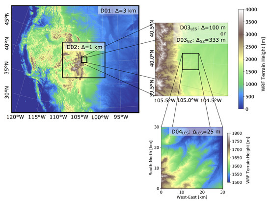
Figure 1.
Simulation domains used. The first two domains (D01 and D02, shown on the left) are the same for all simulations performed. The third largest domain (D03) is approximately the same extent for both simulations, but two different horizontal grid spacings are used: m for gray-zone simulations and 100 m for the reference simulation RLES. The fourth domain (D04) has a grid spacing of m and is only included in the RLES case.
All simulations consider real-world, full-physics, WRF-based conditions (i.e., not idealized). The initial and boundary conditions provided to all simulations are from hourly Rapid Refresh [28] 5-hour forecasts produced by the National Center for Environmental Prediction. The grid spacing of this dataset is approximately 13.2 km. All simulations are run with 73 vertical levels, approximately 12 of which are below 200 m (and 30 within the first kilometer above ground level). Simulations are performed for March 2015 because of the availability of measurements collected through the experimental planetary boundary layer instrumentation assessment (XPIA) field campaign [29]. These measurements were used to validate the simulations performed for this month [23], and 5 days were chosen based on the model performance in simulating wind speed, wind direction and air temperature near the ground: 20, 21, 28, 29 and 30 March. The simulations analyzed here consider the convective portion of the diurnal cycle for these 5 days. Data are considered between 1400 and 2400 UTC (0800 to 1800 local time) every 10 min. For the days considered, the sunrise and sunset times are ∼1256 UTC (∼0656 LT) and ∼0117 UTC (∼1917 LT), respectively. For each convective period, the mesoscale (i.e., the two largest domains) is run for 36 h. The smaller nests are initialized at hour 24, running for a total of 12 h: 2 h for spin up and 10 h for the final analysis. This setup has been previously demonstrated in a validation study that compared resolved turbulence quantities against sonic anemometer data from the XPIA campaign [23].
The cell-perturbation method [30,31] is used in RLES to ensure the development of small-scale turbulence as the mesoscale flow structures in the second domain (1-km grid spacing) are passed to the microscale LES in the third domain (100-m grid spacing). With this method, the lateral boundary conditions are perturbed between the third vertical level and the one corresponding to ∼70% of the boundary layer height. The magnitude of this perturbation and its vertical extent are computed a priori for each convective cycle, based on the physical state of the atmospheric boundary layer according to the mesoscale spin up simulations [32]. The fourth, innermost RLES domain does not undergo any cell perturbation. The third domain in the gray-zone simulations (VLES, MYNN, YSU, SH) is also perturbed in the same manner as the RLES to ensure consistency across simulation approaches and instigate the development of under-resolved convective structures.
Whenever the domain is run in LES mode (i.e., the two inner domains in RLES and the innermost domain in VLES), a three-dimensional turbulent kinetic energy (TKE) 1.5-order closure is used [16]. An isotropic subgrid length scale is used in the RLES simulation approach, where the horizontal grid spacing of the LES domains is ≤100 m and comparable in all directions. For nonisotropic grids, different length scales are used. Note that in WRF, the isotropic assumption results in a uniform length scale that is proportional to the grid sizes across the three directions, , , and . These length scales are used to compute horizontal and vertical eddy diffusivities of momentum and heat, thereby directly affecting momentum and heat mixing. In nonisotropic conditions, different length scales are used for horizontal and vertical diffusion. In contrast to the LES setup, when the boundary layer is parameterized, horizontal diffusion is accounted for with a first-order Smagorinsky closure while vertical diffusion is assumed to be one-dimensional and treated via the selected PBL scheme (i.e., MYNN, YSU or SH).
The four gray-zone simulation approaches only differ in the way that the boundary layer is treated, as summarized in Table 1. By comparing these approaches with RLES, we seek to quantify how these treatments affect simulated flow structures. As previously stated, one method treats the gray zone as a nonisotropic VLES. A second method uses the well-established MYNN PBL scheme [27]—the same used in the two largest domains in all simulation approaches to model the mesoscale fields. A third method uses the YSU PBL scheme [33]. The main difference between YSU and MYNN is that the latter is a local scheme, meaning that vertical transport is achieved with diffusion across adjacent grid cells via small-scale turbulence (the counter-gradient eddy viscosity approach). Conversely, YSU is a nonlocal scheme that accounts for vertical transport via strong updrafts of organized structures, such as convective cells and rolls. A second difference is that MYNN uses a 1.5-order closure (i.e., it uses a prognostic equation for SGS TKE to parameterize the turbulence diffusivities of momentum, heat and other scalars), whereas YSU implements a first-order closure. The third PBL scheme considered is referred to as SH and represents a modification of YSU for simulating convection at intermediate, gray-zone resolutions [21], and it was developed based on a set of idealized simulations of convective boundary layers performed with WRF-LES.

Table 1.
Summary of the five simulation approaches considered.
3. Analysis Methods
3.1. Spatial Extent and Resolution
The analysis is based on a direct comparison of the five simulation approaches. To make all of them comparable, the gray-zone domains (which are larger in extent, see Table 1), are first clipped to match the area covered by the RLES innermost domain. Then, all five datasets are filtered in spectral space so that the higher-resolution RLES fields can be directly compared to the coarser gray zone fields. This way, differences between simulation approaches are independent of grid spacing and strictly the result of different PBL parameterizations in the simulations.
An example of the filtering process is given in Figure 2 for potential temperature perturbation fields. The filtering method applied uses a hybrid uniform-Hanning window and a Butterworth filter. The window function is uniform at the center of the domain to avoid smoothing out the flow fields of interest and follows a Hanning function along the edges. After windowing, the following Butterworth filter is applied to the flow fields,
where (m) are the wave numbers, (m) is the cut-off wave number for the filter and n is the order of the filter. Herein, km and . This value ensures that only the modes that are fully resolved in all simulation approaches are considered in the analysis. For the simulations performed, the effective model resolution is because of the hybrid-order advection scheme with improved spectral resolution utilized [34].
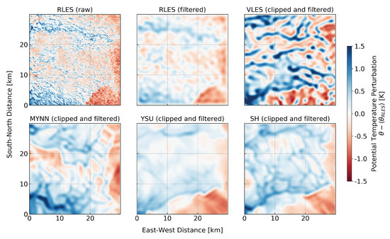
Figure 2.
Example of potential temperature perturbation fields (at model level 6, ∼90 m above ground for this time) for each simulation approach. Data are valid for 28 March 2015, at 17:30 UTC (11:30 LT). RLES fields are shown before and after spatial filtering. Gray-zone fields (VLES, MYNN, YSU, SH) are shown after clipping and filtering. All fields are filtered at m.
3.2. Convective Regime Categorization
As previously mentioned, each of the five daytime cycles is analyzed for 10 h (between 0800 and 1800 LT), with an output frequency of 10 min. Therefore, a total of 300 snapshots is available for analysis for each simulation approach across the 5 days. Each of these snapshots is placed into one of two categories: convective cells; and transition regime or convective rolls. These regimes are exemplified with vertical velocity fields in Figure 3.
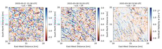
Figure 3.
Instantaneous vertical velocity fields (∼100 m above ground) obtained from the innermost domain of the reference simulation RLES and shown for a box centered in the innermost domain and spanning 10 km × 10 km horizontally. These examples highlight differences in the turbulence structures depending on atmospheric stability: cell-dominated convection (left), transition (center) and roll (right) regimes.
The classification of each flow state into one of the two regimes is based on the relative magnitude of the boundary-layer height () and the Obukhov length (L): . This boundary layer height is taken from the mesoscale parent domain of each dataset being analyzed (D02, the second largest domain shown in Figure 1) as the value computed by the MYNN boundary layer parameterization, and it is shown in Figure 4c. This choice ensures consistency in the calculations, as the mesoscale parent domain has the exact same configuration for all simulation approaches. The Obukhov length is calculated from the RLES fields as
where the friction velocity (m s) is a diagnostic of the model (shown in Figure 4a), the potential temperature (K) is considered at the first model level ( m above ground), k is the von Karman constant (), g (m s) is the gravitational acceleration, and Q (W m s) is the kinematic heat flux computed from the model diagnostics for sensible and latent heat fluxes at the surface (shown in Figure 4b) and air density.
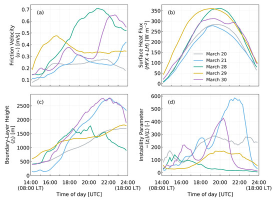
Figure 4.
Diurnal evolution of friction velocity, upward surface heat flux, boundary layer height and instability parameter. Shown for each diurnal cycle considered in the analysis and obtained from the reference simulation RLES. The values are spatial averages within a box that is centered in the innermost domain and spans 15 km × 15 km horizontally.
Because these are full-physics, real-case simulations covering a relatively large domain, the resulting estimates for boundary layer height, momentum fluxes and heat fluxes are typically heterogeneous. To obtain a single estimate of these parameters at each time, the values obtained are averaged in space over a 15 km × 15 km area, with the midpoint at the center of the innermost domain. The final values obtained and the resulting instability parameter are shown in Figure 4. A clear diurnal cycle can be seen for the 5 days in the heat flux and boundary layer height values. The diurnal evolution of friction velocity is less consistent, leading to pronounced differences across the different days. These differences propagate to estimates of the instability parameter , which are different depending on the day. The magnitude of values is overall high, indicating that most of the simulated flow is comprised of convective cells (as opposed to convective rolls or a transition regime). There is no universal cut-off value of that can be used to clearly distinguish between roll and cell regimes under all conditions [35]. For the purposes of this work, we adopt the previously used value of [36]. This cut-off reveals that 90% (Figure 5) of the simulated data (269 out of 300 snapshots) falls within the convective cell category (). To ensure statistical significance of the results, the analysis presented throughout this article will consider only the snapshots that fall within this regime.
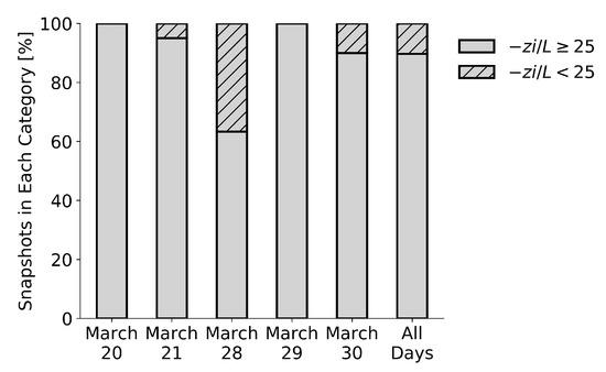
Figure 5.
Percentage of simulation snapshots that falls into each of two categories: instability parameter (convective cell regime) and (transition or convective-roll regime). Shown for each simulated day and for all days combined.
3.3. Simulation Performance Assessment
The performance of each gray-zone simulation approach is assessed relative to the RLES fields. This assessment is done considering planar averages of quantities throughout the vertical extent of the atmospheric boundary layer and horizontal planes at fixed heights. No vertical interpolation is performed, and all quantities are kept in the terrain-following WRF coordinates. For a given time and simulation approach, the height of a model level is taken as the horizontal average of the height values , where i represents the coordinate along west-east, j along south-north, k the terrain-following model level and t time. These averages consider a domain-centered area that spans 30 km along the i and j directions. Because interpolation is not performed, the planar averages and horizontal planes are not strict planes but approximate planes. This assumption is reasonable given the relatively simple terrain in the area of focus: a maximum elevation change of 300 m across 30 km.
For the vertical assessment, we consider the root-mean-squared error (RMSE) of planar-averaged (i.e., horizontally averaged) quantities. To obtain these error metrics, each quantity of interest is averaged horizontally over an area that is 15 km × 15 km to yield . At each time, the RMSE of the vertical profile is computed relative to RLES by considering points where . Finally, the vertical median of these values is computed, resulting in a time series of vertically averaged RMSE for each quantity of interest and simulation strategy. To complement the RMSE analysis, the median of the bias across the atmospheric boundary layer is also considered, where positive values represent an overestimation of the simulation relative to RLES.
For the horizontal assessment, flow fields are compared qualitatively with contour plots and quantitatively in Fourier space. The one-dimensional energy spectra considered in the analyses are obtained by mapping the two-dimensional fast Fourier transform (FFT) from Cartesian to polar coordinates and then averaging the FFT signal power across azimuths. The azimuthally averaged power is therefore given as a function of radial wavenumber . The spectral range considered is limited to , where was used to filter the flow fields as described in Section 3.1. An example of the azimuthally averaged spectra showing the entire wavelength range and zooming in on the region of interest is shown in Figure 6.
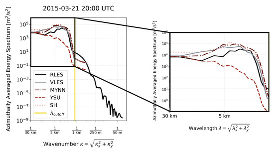
Figure 6.
Example of azimuthally averaged power spectra of vertical velocity perturbations for the five simulation approaches. The left panel shows the entire wavenumber range, and the right panel shows the wavelength range considered in the analysis, starting at .
4. Results
The objective of this section is to identify and quantify weaknesses and strengths of the four gray-zone simulation approaches considered. The model performance for each approach is determined relative to the reference LES simulation, RLES. First, an overall performance analysis is carried out with statistical distributions of errors that consider horizontally averaged atmospheric quantities throughout the atmospheric boundary layer. This analysis provides insight into vertically integrated model performance in terms of the magnitude of several quantities. Next, the simulation approaches are evaluated regarding the spatial structure of turbulence via qualitative assessments of the flow fields and a quantitative description of energy across scales. For this second assessment, specific simulation times are chosen to exemplify scenarios that highlight the skills and shortcomings of the different modeling techniques. Because these are not idealized simulations of specific atmospheric states, we do not expect a single simulation approach to outperform all others for all quantities of interest. Rather, we seek to identify which approaches work well under which convective conditions when simulating real, complex atmospheric scenarios arising from dynamic, heterogeneous forcing conditions.
4.1. Shin-Hong Grid Dependence
This section provides quantitative evidence on the motivation for comparing the YSU and SH parameterizations. It is important to keep in mind that these two approaches will only differ at certain times. More specifically, SH incorporates two grid-dependency functions that scale the magnitude of the parameterized vertical heat transport depending on the ratio between horizontal grid spacing and boundary layer height, . One of these functions acts on local transport ( in Figure 7) and the other on nonlocal transport ( in Figure 7). These two functions are active for the majority of the times simulated herein but with different magnitudes. The effect of these functions on the simulated flow fields increases as the day progresses, as shown in Figure 7b. For more detail on the formulation of the SH scheme, the reader is referred to [21].
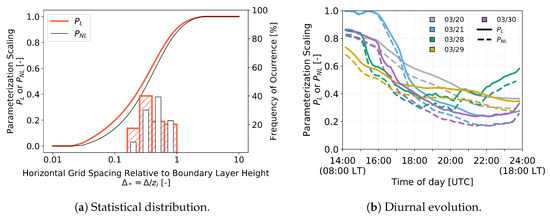
Figure 7.
Values of the Shin-Hong parameterization grid-dependency functions PL and PNL for the five convective cycles simulated for this work. Left panel (a) shows the two functions (lines) and the frequency of occurrence of function values during the analyzed simulation times (bars). Right panel (b) shows the diurnal evolution of the two functions separated by day.
4.2. Spatially Averaged Errors
The statistics of RMSE values for each quantity and simulation approach are shown in Figure 8. The main overall results from this analysis are that VLES yields the largest errors and YSU and SH the smallest errors for most quantities of interest. The exceptions to this are (i) vertical velocity variance, for which the MYNN distribution presents a similar median error but larger spread and tail than VLES; and (ii) potential temperature, for which MYNN presents the lowest median error and an error spread that is comparable to YSU and SH.
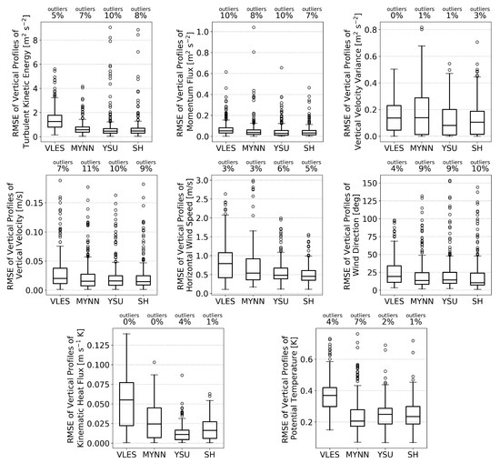
Figure 8.
Distribution of RMSE time series computed from vertical profiles of horizontally averaged turbulent kinetic energy, momentum flux, vertical velocity variance, vertical velocity, horizontal wind speed and direction, heat flux and potential temperature. Whisker plots show 25th, 50th and 75th quantiles. The circles extending out from the whisker plots represent the distribution outliers. The percent values in each figure quantify the percentage of outliers rounded to the nearest integer.
All simulation approaches show normally distributed errors for vertical velocity variance and heat flux, with outliers staying below 4%. For these two quantities, YSU has the lowest mean error, followed by SH and MYNN. Although the majority of error values are low in magnitude for TKE and momentum flux, these two quantities show a slightly larger number of outliers, between 5% and 10%. As previously mentioned, 269 snapshots are being considered in this analysis, and the 10% figure represents 27 snapshots of simulated flow fields. In the next section, these outliers will be investigated in more detail. A large number of outliers is also observed for vertical velocity and wind direction. Fewer outliers are observed for horizontal wind speed, with SH performing the best, followed closely by YSU and MYNN.
The mean bias in Figure 9 complements the RMSE analysis by revealing trends in under vs. overestimation for the turbulence quantities considered. Momentum flux is not shown here because its mean bias is close to zero for all simulation strategies. The TKE, vertical velocity variance and heat flux bias statistics reveal that YSU tends to underestimate the turbulent fluxes, whereas the other three simulation approaches (VLES, MYNN, SH) overestimate them. These sign differences are especially important when comparing YSU and SH: while the median RMSE is very similar for these two approaches, the difference in sign observed for the median bias indicates that the turbulent flow fields being simulated by these two approaches likely exhibit substantial physical differences. The spatial structure of these turbulence structures will be examined in more detail in the following sections.
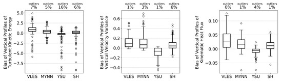
Figure 9.
Distribution of bias time series computed from vertical profiles of horizontally averaged turbulent kinetic energy, vertical velocity variance and heat flux. Whisker plots show 25th, 50th and 75th quantiles. The circles extending out from the whisker plots represent the distribution outliers. The percent values in each figure quantify the percentage of outliers rounded to the nearest integer.
4.3. Turbulent Energy Spectra
In this section, we complement the overall error analysis by considering power spectra of turbulent fluxes. The vertical velocity spectra for each of the cases (Figure 10) exhibit very clear trends that are also visible in the and cospectra (not shown).
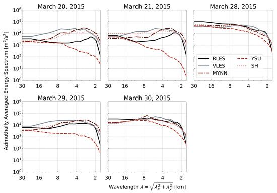
Figure 10.
Diurnal average (0800-1800 LT) of azimuthally averaged power spectra for vertical velocity perturbations at .
First, note the difference in spread across simulation strategies for the different days: substantially more variation can be observed for 20, 21 and 29 March than for 28 and 30 March. These last 2 days have more energy at large scales (i.e., 30 km 8 km) and the largest number of snapshots with (Figure 5), both of which indicate the prevalence of convective rolls or a transition state over thermally induced cells. Note that the daily-averaged spectra shown here do not consider the snapshots with , which were removed from the analysis after the convective regime categorization (Section 3.2). The fact that this low spread across simulations remains even after categorizing the data indicates that these 2 days are driven by different atmospheric forcing. This can be confirmed by visual inspection of the turbulence structure and horizontal wind fields at the same height that the spectra were computed. These flow fields, shown in Figure 11 and Figure 12, represent the last simulated time on 28 March for which (i.e., the last time for this day that is included in the analysis). The vertical velocity turbulence structure reveals a complex convective state, with small structures to the north and large roll-like shapes extending along the northwest-southeast direction. The wind direction is homogeneous throughout the domain and the wind speed field reveals a large-scale, high-wind feature traversing the domain along the northwest-southeast direction. These features are evidence that large-scale atmospheric structures, likely triggered by flow over terrain to the west (Figure 1), are the dominating features during these 2 days. These larger-scale systems mask the effects of smaller-scale, radiative-driven convection that would otherwise be noticeable in the flow fields and visible in the spectra as an energy peak near km (as observed for 20, 21 and 29 March in Figure 10).
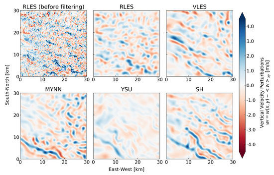
Figure 11.
Contours of vertical velocity perturbations at for all simulation strategies on 28 March, 20:10 UTC (14:10 LT). This is the last time considered in the analysis of 28 March, as determined by the convective regime categorization. For completeness, RLES is shown before and after spatial filtering.
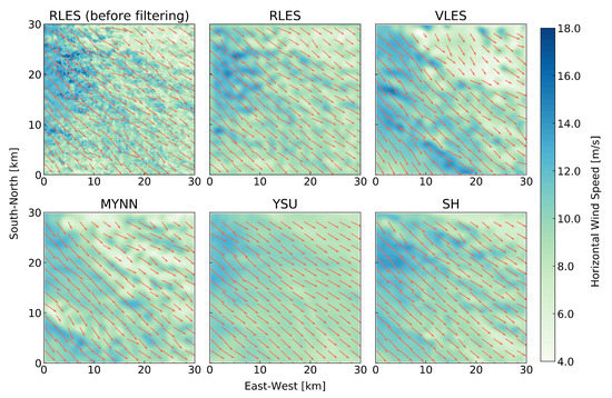
Figure 12.
Contours of horizontal wind speed and wind direction vectors at for all simulation strategies on 28 March, 20:10 UTC (14:10 LT). This is the last time considered in the analysis of 28 March, as determined by the convective regime categorization. For completeness, RLES is shown before and after spatial filtering.
In addition, what is made evident from the spectra in Figure 10 is the consistent underestimation of turbulent energy by YSU, especially for the more convective days (20, 21 and 29 March). This outcome is consistent with previous work [21], which pointed out that YSU can overestimate the magnitude of larger-scale, nonlocal transport for certain convective conditions when the model grid spacing is in the gray zone. This overestimation leaves little energy for resolved motions, leading to a larger dissipation, and the turbulence content ends up being systematically underpredicted, as shown in Figure 10 and consistent with the bias distribution of TKE, vertical velocity and heat flux presented in Figure 9. The results shown herein confirm that this issue is substantially mitigated with the scale-aware SH parameterization. To further illustrate this point, Figure 13 provides a quantitative estimate of the errors of each gray-zone simulation strategy in terms of spectral energy content. The spectra are computed for each snapshot, the area under the energy curve is integrated and a percent error relative to RLES is computed for each simulation approach at each time (i.e., 269 snapshots representing all cases combined). The values shown in Figure 13 present a curve fit to the empirical probability distribution of the time series of percent error values obtained for the three turbulent quantities considered. Note that the large magnitude of the percent errors is simply a result of the magnitude of the values being compared, on the order of to m s. This analysis reveals that the underestimation of turbulence by YSU is even more pronounced for momentum and heat flux. Although SH still under or overestimates the energy content at times, the distribution of errors is centered close to 0%. In addition, SH has a shorter overprediction tail than MYNN and VLES for the three quantities.
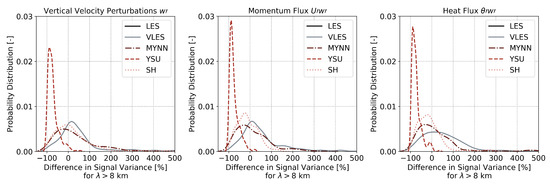
Figure 13.
Curve-fitted histogram for time series of errors (%) in energy (co)spectra, at , integrated for km and shown for vertical velocity perturbations, ; momentum flux, ; and heat flux, .
Contrary to the behavior of YSU, VLES largely overestimates the turbulence energy content for these highly convective days (20, 21 and 29 March). This can be observed from the daily-averaged spectra (Figure 10) and spectral energy error distributions (Figure 13). This observation is also consistent with previous work [37], which pointed out that coarse LES fail to dissipate energy at a realistic rate, leading to an accumulation of energy along the wavenumber spectrum. In other words, because too little energy is dissipated by the SGS parameterization, there is too much energy available for resolved motions.
To complement the energy spectra analysis, Figure 14 and Figure 15 show contours of vertical velocity and wind speed for a highly convective snapshot on 21 March at 2100 UTC, chosen based on the peak values in (Figure 4d). These figures illustrate the performance of each simulation strategy in terms of reproducing the spatial structure of the flow fields in the horizontal direction. The RLES vertical velocity fields show clear convective cell structures (unlike the 28 March flow field shown in Figure 11). Despite an overestimation in the magnitude of these up and downdrafts, as well as some overprediction of the cell’s wavelength (peak of energy spectra in Figure 10), VLES, MYNN and SH are able to reproduce the spatial structure of the turbulent field. In contrast, YSU underestimates the magnitude of the perturbations and fails to simulate the cell-like structures present in the reference simulation. As a result, the YSU wind speed and direction fields are unrealistically homogeneous and the small-scale, terrain-induced, high-speed flows are not reproduced.
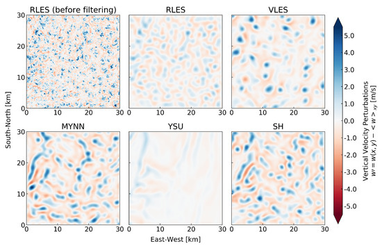
Figure 14.
Contours of vertical velocity perturbations at for all simulation strategies on 21 March, 2100 UTC (1500 LT). This time represents a peak in , as shown in Figure 4d. For completeness, RLES is shown before and after spatial filtering.
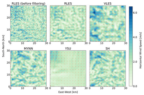
Figure 15.
Contours of horizontal wind speed and wind direction vectors at for all simulation strategies on 21 March, 2100 UTC (1500 LT). This time represents a peak in , as shown in Figure 4d. For completeness, RLES is shown before and after spatial filtering.
4.4. Horizontally-Averaged Vertical Profiles
Despite failing to reproduce the magnitude and structure of turbulence at , horizontally-averaged vertical profiles reveal that YSU can outperform the other gray-zone simulation strategies at certain times and heights when considering integrated error statistics. To exemplify this point, Figure 16 shows vertical profiles of several mean and turbulent quantities for the same time as Figure 14 and Figure 15. These figures elucidate the apparent contradiction resulting from the previous analyses for YSU: a good performance in terms of mean errors and a poor performance in terms of turbulence magnitude and structure. The low RMSE and bias for YSU (Section 4.2) result from cases in which RLES has fairly low turbulence values, as shown in the four bottom subpanels in Figure 16. During these cases, the low-turbulence YSU is often closer to the RLES profile than the more turbulent VLES, MYNN and SH approaches. This example does not contradict or override the results from the previous sections. Because these are real and not idealized WRF simulations, different simulation approaches will perform better for different quantities of interest at different times. Therefore, specific snapshots cannot provide overall simulation performance diagnostics. Instead, the contours and vertical profiles of specific times are included to illustrate the simulated physical states that lead to certain results.
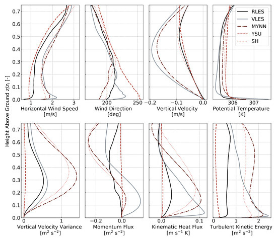
Figure 16.
Vertical profiles of horizontally averaged quantities between on 21 March, 2100 UTC (1500 LT). This time represents a peak in , as shown in Figure 4d. Horizontal averages consider an area that extends 15 km × 15 km.
5. Discussion
The currently available methods for simulating atmospheric boundary layers at gray-zone scales are traditional one-dimensional parameterizations, scale-aware parameterizations and coarse LES. Here, we evaluated the performance of these different methods relative to highly resolved LES. In addition to coarse LES, we considered three PBL parameterizations available in WRF: a traditional local scheme (MYNN), a nonlocal scheme (YSU) and a scale-aware scheme (Shin-Hong (SH)). The convective portion of five diurnal cycles in March 2015 was simulated, and the times corresponding to a convective-cell regime were considered in the analysis.
For days in which turbulence scales are large and topography-induced flows wash out radiation-driven convective structures, all simulation approaches perform reasonably well. In contrast, the differences across simulation strategies are pronounced for highly convective days. For these days, SH presents the overall best performance and VLES the worst. In terms of turbulence energy spectra, all simulations fail to reproduce the peak energy values for wavelengths of ∼2 km, as observed in RLES for 20 and 21 March and to a lesser extent, for 29 March.
The analysis revealed that the nonlocal YSU scheme consistently underestimates the magnitude of turbulence, especially for wavelengths greater than 8 km. In addition, YSU often fails to reproduce the spatial structure of cellular convection. However, the spatially integrated error analysis indicated that this scheme might be acceptable for applications that do not focus on turbulence, because overall error magnitudes are comparable to the other simulation approaches.
The scale-aware SH scheme, which is a modification of YSU for simulating convection at intermediate scales, performed better than YSU at reproducing the magnitude and structure of turbulence, especially for the three most convective days: 20, 21 and 29 March. This result is observed from energy spectra and horizontal contours of flow fields but is not evident in the overall error metrics that are similar for YSU and SH. Despite representing an improvement in simulating turbulence at gray-zone scales, SH seems to have overcompensated for the effects of grid spacing on the turbulent transport and overly reduced the amount of energy dissipation, leading to an overprediction of turbulent energy in some cases.
The local MYNN scheme had overall slightly larger errors than YSU and SH. Although daily-averaged spectra indicate a similar magnitude of energy overestimation for SH and MYNN, time-resolved differences reveal that MYNN overpredicts the energy content in vertical velocity fluctuations, momentum flux and heat flux to a larger extent than SH. In terms of spatial structure and magnitude of fluctuations, MYNN outperformed YSU. As already mentioned, the worst performance was observed for VLES, the coarse LES approach. In addition to presenting the largest overall errors, VLES also consistently overestimated the magnitude of turbulence across scales for the three most convective days.
6. Conclusions
This work revealed that users interested in subkilometer simulations within WRF should refrain from coarse LES and favor the scale-aware parameterization Shin-Hong over other traditional alternatives (MYNN and YSU one-dimensional PBL schemes). These results are based on analyses of the finest nest and not the parent domain used to generate boundary conditions for the nest. For parent domains, previous work [9] found that turbulence modeling choices at the gray zone have little effect on the flow simulated by the finer nest. The fact that Shin-Hong performed better than YSU indicates a promising avenue for schemes that take the grid spacing and boundary layer height into account when computing subgrid-scale transport. However, the fact that Shin-Hong overcompensated this scale dependence indicates that more work needs to be done to develop turbulence modeling alternatives adequate for gray-zone resolutions. For example, we expect extensions to the Shin-Hong scale-aware scheme including subgrid-scale momentum fluxes and horizontal flux divergence terms to contribute to a more robust behavior across gray-zone resolutions. With the growing use of WRF at subkilometer scales across a broad user group, the need for a robust gray-zone modeling solution is urgent to ensure that research and technology decisions are based on reliable results. This modeling solution could also take the form of an adaptation of three-dimensional isotropic turbulence schemes [25,38,39].
As new or improved solutions are proposed, we suggest that they be evaluated against existing alternatives following the procedure presented in this work. In addition, future work should leverage observational datasets, be expanded to a longer simulation time period and consider the spatial structure of turbulence in more detail and at more heights above ground. For example, analyses focused on near-ground mean and turbulent flow would directly benefit wind energy research and industry, which is quickly adopting subkilometer atmospheric modeling capabilities.
Author Contributions
Conceptualization, methodology, formal analysis, writing—review & editing, P.D. and D.M.-E.; data curation, investigation, validation, visualization, writing—original draft, P.D.; resources, supervision, D.M.-E. All authors have read and agreed to the published version of the manuscript.
Funding
This work was authored (in part) by the National Renewable Energy Laboratory, operated by Alliance for Sustainable Energy, LLC, for the U.S. Department of Energy (DOE) under Contract No. DE-AC36-08GO28308. Funding provided by the U.S. Department of Energy Office of Energy Efficiency and Renewable Energy Wind Energy Technologies Office. The views expressed in the article do not necessarily represent the views of the DOE or the U.S. Government. The U.S. Government retains and the publisher, by accepting the article for publication, acknowledges that the U.S. Government retains a nonexclusive, paid-up, irrevocable, worldwide license to publish or reproduce the published form of this work, or allow others to do so, for U.S. Government purposes. All the simulations were performed using high-performance computing support from Cheyenne (https://doi.org/10.5065/D6RX99HX) provided by the National Center for Atmospheric Research (NCAR) Computational and Information Systems Laboratory, sponsored by the National Science Foundation. The specific computing time was provided by the NCAR Strategic Capability Computing Grant “Coupled mesoscale to microscale simulations using the Weather Research and Forecasting model” (NRAL0016).
Conflicts of Interest
The authors declare no conflict of interest.
References
- Powers, J.G.; Klemp, J.B.; Skamarock, W.C.; Davis, C.A.; Dudhia, J.; Gill, D.O.; Coen, J.L.; Gochis, D.J.; Ahmadov, R.; Peckham, S.E.; et al. The Weather Research and Forecasting model: Overview, system efforts and future directions. Bull. Am. Meteorol. Soc. 2017, 98, 1717–1737. [Google Scholar] [CrossRef]
- Skamarock, W.C.; Klemp, J.B. A time-split nonhydrostatic atmospheric model for weather research and forecasting applications. J. Comput. Phys. 2008, 227, 3465–3485. [Google Scholar] [CrossRef]
- Mirocha, J.D.; Kosovic, B.; Aitken, M.L.; Lundquist, J.K. Implementation of a generalized actuator disk wind turbine model into the Weather Research and Forecasting model for large-eddy simulation applications. J. Renew. Sustain. Energy 2014, 6, 013104. [Google Scholar] [CrossRef]
- Simpson, C.; Sharples, J.; Evans, J. Resolving vorticity-driven lateral fire spread using the WRF-Fire coupled atmosphere-fire numerical model. Nat. Hazards Earth Syst. Sci. 2014, 14. [Google Scholar] [CrossRef]
- Wang, H.; Skamarock, W.C.; Feingold, G. Evaluation of scalar advection schemes in the Advanced Research WRF model using large-eddy simulations of aerosol-cloud interactions. Mon. Weather. Rev. 2009, 137, 2547–2558. [Google Scholar] [CrossRef]
- Sueki, K.; Yamaura, T.; Yashiro, H.; Nishizawa, S.; Yoshida, R.; Kajikawa, Y.; Tomita, H. Convergence of convective updraft ensembles with respect to the grid spacing of atmospheric models. Geophys. Res. Lett. 2019, 46, 14817–14825. [Google Scholar] [CrossRef]
- Wyngaard, J.C. Toward numerical modeling in the “Terra Incognita”. J. Atmos. Sci. 2004, 61, 1816–1826. [Google Scholar] [CrossRef]
- Haupt, S.E.; Kosovic, B.; Shaw, W.; Berg, L.K.; Churchfield, M.; Cline, J.; Draxl, C.; Ennis, B.; Koo, E.; Kotamarthi, R.; et al. On bridging a modeling scale gap: Mesoscale to microscale coupling for wind energy. Bull. Am. Meteorol. Soc. 2019, 100, 2533–2550. [Google Scholar] [CrossRef]
- Rai, R.K.; Berg, L.K.; Kosović, B.; Haupt, S.E.; Mirocha, J.D.; Ennis, B.L.; Draxl, C. Evaluation of the impact of horizontal grid spacing in terra incognita coupled mesoscale-microscale simulations using the WRF framework. Mon. Weather Rev. 2019, 147, 1007–1027. [Google Scholar] [CrossRef]
- Jeworrek, J.; West, G.; Stull, R. Evaluation of cumulus and microphysics parameterizations in WRF across the convective gray zone. Weather Forecast 2019, 34, 1097–1115. [Google Scholar] [CrossRef]
- Kealy, J.C.; Efstathiou, G.A.; Beare, R.J. The onset of resolved boundary-layer turbulence at grey-zone resolutions. Bound. Layer Meteorol. 2019, 171, 31–52. [Google Scholar] [CrossRef]
- Honnert, R.; Masson, V.; Couvreux, F. A diagnostic for evaluating the representation of turbulence in atmospheric models at the kilometric scale. J. Atmos. Sci. 2011, 68, 3112–3131. [Google Scholar] [CrossRef]
- Honnert, R. Representation of the grey zone of turbulence in the atmospheric boundary layer. Adv. Sci. Res. 2016, 13, 63–67. [Google Scholar] [CrossRef]
- Kolmogorov, A.N. Dissipation of energy in locally isotropic turbulence. Dokl. Akad. Nauk SSSR 1941, 32, 16–18. [Google Scholar]
- Smagorinsky, J. General circulation experiments with the primitive equations. Mon. Weather Rev. 1963, 91, 99–164. [Google Scholar] [CrossRef]
- Lilly, D.K. The representation of small-scale turbulence in numerical simulation experiments. IBM Form 1966. [Google Scholar] [CrossRef]
- Eriksson, O.; Lindvall, J.; Breton, S.P.; Ivanell, S. Wake downstream of the Lillgrund wind farm-A comparison between LES using the actuator disc method and a wind farm parametrization in WRF. J. Phys. 2015, 625, 012028. [Google Scholar] [CrossRef]
- Jiménez, P.A.; Navarro, J.; Palomares, A.M.; Dudhia, J. Mesoscale modeling of offshore wind turbine wakes at the wind farm resolving scale: A composite-based analysis with the Weather Research and Forecasting model over Horns Rev. Wind Energy 2015, 18, 559–566. [Google Scholar] [CrossRef]
- Cui, C.; Bao, Y.; Yuan, C.; Li, Z.; Zong, C. Comparison of the performances between the WRF and WRF-LES models in radiation fog–A case study. Atmos. Res. 2019, 226, 76–86. [Google Scholar] [CrossRef]
- Xue, L.; Chu, X.; Rasmussen, R.; Breed, D.; Geerts, B. A case study of radar observations and WRF LES simulations of the impact of ground-based glaciogenic seeding on orographic clouds and precipitation. Part II: AgI dispersion and seeding signals simulated by WRF. J. Appl. Meteorol. Climatol. 2016, 55, 445–464. [Google Scholar] [CrossRef]
- Shin, H.H.; Hong, S.Y. Representation of the subgrid-scale turbulent transport in convective boundary layers at gray-zone resolutions. Mon. Weather Rev. 2015, 143, 250–271. [Google Scholar] [CrossRef]
- Ito, J.; Niino, H.; Nakanishi, M.; Moeng, C.H. An extension of the Mellor–Yamada model to the Terra Incognita zone for dry convective mixed layers in the free convection regime. Bound. Layer Meteorol. 2015, 157, 23–43. [Google Scholar] [CrossRef]
- Muñoz-Esparza, D.; Sharman, R.; Sauer, J.; Kosović, B. Toward low-level turbulence forecasting at eddy-resolving scales. Geophys. Res. Lett. 2018, 45, 10. [Google Scholar] [CrossRef]
- Ching, J.; Rotunno, R.; LeMone, M.; Martilli, A.; Kosovic, B.; Jimenez, P.A.; Dudhia, J. Convectively induced secondary circulations in fine-grid mesoscale numerical weather prediction models. Mon. Weather Rev. 2014, 142, 3284–3302. [Google Scholar] [CrossRef]
- Honnert, R. Grey-zone turbulence in the neutral atmospheric boundary layer. Bound. Layer Meteorol. 2018. [Google Scholar] [CrossRef]
- Zhou, B.; Simon, J.S.; Chow, F.K. The convective boundary layer in the Terra Incognita. J. Atmos. Sci. 2014, 71, 2545–2563. [Google Scholar] [CrossRef]
- Nakanishi, M.; Niino, H. An improved Mellor–Yamada level-3 model: Its numerical stability and application to a regional prediction of advection fog. Bound.-Layer Meteorol. 2006, 119, 397–407. [Google Scholar] [CrossRef]
- Benjamin, S.G.; Weygandt, S.S.; Brown, J.M.; Hu, M.; Alexander, C.R.; Smirnova, T.G.; Olson, J.B.; James, E.P.; Dowell, D.C.; Grell, G.A.; et al. A North American hourly assimilation and model forecast cycle: The Rapid Refresh. Mon. Weather Rev. 2015, 144, 1669–1694. [Google Scholar] [CrossRef]
- Lundquist, J.K.; Wilczak, J.M.; Ashton, R.; Bianco, L.; Brewer, W.A.; Choukulkar, A.; Clifton, A.; Debnath, M.; Delgado, R.; Friedrich, K.; et al. Assessing state-of-the-art capabilities for probing the atmospheric boundary layer: The XPIA field campaign. Bull. Am. Meteorol. Soc. 2016, 98, 289–314. [Google Scholar] [CrossRef]
- Muñoz-Esparza, D.; Kosović, B.; van Beeck, J.; Mirocha, J. A stochastic perturbation method to generate inflow turbulence in large-eddy simulation models: Application to neutrally stratified atmospheric boundary layers. Phys. Fluids 2015, 27, 035102. [Google Scholar] [CrossRef]
- Muñoz-Esparza, D.; Kosović, B.; Mirocha, J.; Beeck, J.V. Bridging the transition from mesoscale to microscale turbulence in numerical weather prediction models. Bound. Layer Meteorol. 2014, 153, 409–440. [Google Scholar] [CrossRef]
- Muñoz-Esparza, D.; Kosović, B. Generation of inflow turbulence in large-eddy simulations of nonneutral atmospheric boundary layers with the cell perturbation method. Mon. Weather Rev. 2018, 146, 1889–1909. [Google Scholar] [CrossRef]
- Hong, S.Y.; Noh, Y.; Dudhia, J. A new vertical diffusion package with an explicit treatment of entrainment processes. Mon. Weather Rev. 2006, 134, 2318–2341. [Google Scholar] [CrossRef]
- Kosovic, B.; Muñoz-Esparza, D.; Sauer, J. Improving spectral resolution of finite difference schemes for multiscale modeling applications using numerical weather prediction model. In Proceedings of the 22nd Symposium on Boundary Layers and Turbulence, Salt Lake City, UT, USA, 19 June 2016. [Google Scholar]
- Salesky, S.T.; Chamecki, M.; Bou-Zeid, E. On the nature of the transition between roll and cellular organization in the convective boundary layer. Bound.-Layer Meteorol. 2017, 163, 41–68. [Google Scholar] [CrossRef]
- Weckwerth, T.M.; Horst, T.W.; Wilson, J.W. An observational study of the evolution of horizontal convective rolls. Mon. Weather Rev. 1999, 127, 2160–2179. [Google Scholar] [CrossRef]
- Muñoz-Esparza, D.; Kosović, B.; García-Sánchez, C.; van Beeck, J. Nesting turbulence in an offshore convective boundary layer using large-eddy simulations. Bound. Layer Meteorol. 2014, 151, 453–478. [Google Scholar] [CrossRef]
- Zhang, X.; Bao, J.W.; Chen, B.; Grell, E.D. A three-dimensional scale-adaptive turbulent kinetic energy scheme in the WRF-ARW model. Mon. Weather Rev. 2018, 146, 2023–2045. [Google Scholar] [CrossRef]
- Kosović, B.; Munoz, P.J.; Juliano, T.; Martilli, A.; Eghdami, M.; Barros, A.; Haupt, S. Three-dimensional planetary boundary layer parameterization for high-resolution mesoscale simulations. J. Phys. 2020, 1452, 012080. [Google Scholar] [CrossRef]


© 2020 by the authors. Licensee MDPI, Basel, Switzerland. This article is an open access article distributed under the terms and conditions of the Creative Commons Attribution (CC BY) license (http://creativecommons.org/licenses/by/4.0/).