Effect of Alternate Sprinkler Irrigation with Saline and Fresh Water on Soil Water–Salt Transport and Corn Growth

Abstract

To address freshwater scarcity and the underutilization of low-saline water in the North China Plain, a field study was conducted to evaluate the effects of alternating sprinkler irrigation using saline and fresh water on soil water–salt dynamics and corn growth. Two salinity levels (3 and 5 g·L⁻¹, representing S1 and S2, respectively) and three irrigation strategies—saline–fresh–saline–fresh (F1), saline–fresh (F2), and mixed saline–fresh (F3)—were tested, resulting in six treatments: S1F1, S1F2, S1F3, S2F1, S2F2, and S2F3. S1F1 significantly improved soil water retention at a 30–50 cm depth and reduced surface electrical conductivity (EC) and Na⁺ concentration (p < 0.05). S1F1 also promoted more uniform Mg²⁺ distribution and limited Ca²⁺ loss. Under high salinity (5 g·L⁻¹), surface salt accumulation and ion concentration (Na⁺, Mg²⁺, and Ca²⁺) increased, particularly in S2F3. Corn growth under alternating irrigation (F1/F2) outperformed the mixed mode (F3), with S1F1 achieving the highest plant height, leaf area, grain number, and 100-grain weight. The S1F1 yield surpassed others by 0.4–3.0% and maintained a better ion balance. These results suggest that alternating irrigation with low-salinity water (S1F1) effectively regulates root-zone salinity and improves crop productivity, offering a practical strategy for the sustainable use of low-saline water resources.

1. Introduction

Water resources are crucial for agricultural development. According to the national standard of Hydrogeological Terminology, underground salt water is defined as a type of groundwater with salinity > 2 g·L⁻¹ [1]. Given the abundance of shallow groundwater with low-salinity in China, the utilization of saline and low-saline water has gradually attracted attention [2], but it inevitably brings a large number of salts into the soil, thereby affecting crop yields [3]. The key to using low-saline water for agricultural irrigation is to select a rational irrigation method to address the issue of salt accumulation in the soil and avoid levels that negatively impact crop growth [4].

EC is a key indicator of soil salinity and is widely used to assess the impact of saline water irrigation on soil health. Elevated EC levels due to saline irrigation can increase osmotic stress, reducing water availability to plants and affecting soil microbial activity [5]. For example, Maas and Hoffman [6] demonstrated that soil EC levels above 4 dS·m⁻¹ significantly reduce crop yields due to increased salinity stress, with thresholds varying by crop species. Similarly, Ayers et al. [7] reported that sprinkler irrigation with saline water increases soil EC in the surface layers, particularly under high evaporation conditions, leading to a salt accumulation that can persist without adequate leaching. These studies underscore the importance of monitoring soil EC to understand the dynamics of salt transport and accumulation under different irrigation regimes, which is a central focus of this study.

Saline irrigation significantly influences both soil and plant responses. On one hand, the soil is a living, heterogeneous, and dynamic system that includes physical, chemical, and biological components and their interactions [8]; high-salinity water reduces soil permeability, disrupts soil aggregation by increasing the sodium adsorption ratio (SAR), and accelerates salt accumulation in the surface layers. On the other hand, excess soil salinity hampers root water uptake due to osmotic stress and leads to ion toxicity, notably affecting crop yield and nutrient absorption. These effects vary with irrigation methods, as different techniques influence the movement and accumulation of water and salt in the soil profile. Both domestic and international research and application efforts have been extensively conducted on the use of saline and low-saline water for irrigation [9,10]. Sheng et al. [11] investigated the effects of irrigation with water of different salinities (0, 1.0, 3.0, and 5.0 g·L⁻¹) on soil physical properties and the characteristics of water flow movement. The results showed that high-salinity irrigation water reduces soil permeability and increases the non-uniformity of water flow movement. Yang et al. [12] found that irrigation with low-saline water of various salinity levels leads to salt accumulation in the soil surface layer, while salt accumulation in the deeper soil layers is relatively lower. High salinity in irrigation water affects soil structure and water flow characteristics, resulting in salt accumulation. Sprinkler irrigation is an efficient and widely used irrigation method. He et al. [13] demonstrated that compared with low-saline water drip irrigation, sprinkler irrigation can effectively reduce salt accumulation in the surface soil and promote the migration and leaching of salts to deeper soil layers. Grieve et al. [14] studied the absorption of Na⁺ and Cl⁻ by soybeans under different low-saline water irrigation methods and found that the absorption rate was less than 0.5% under drip and furrow irrigation, while it reached 2% under sprinkler irrigation. Moreover, combination sprinkler irrigation can ensure the stability of the soil structure and uniform water distribution through the coordinated operation of multiple nozzles. Under the action of gravity and soil matrix adsorption forces, water and dissolved salts are delivered to deeper soil layers near the crop roots [15,16]. During the sprinkler irrigation process, the coordinated operation of multiple nozzles ensures high irrigation uniformity and reduces water loss by delivering water directly to the root zone. According to Sun et al. [15] and Chu et al. [16], this method promotes the deep percolation of salts through gravity and soil matrix adsorption forces, while maintaining stable water distribution across the field.

Compared with continuous sprinkler irrigation using low-saline water, alternate sprinkler irrigation—where saline and fresh water are applied in rotation (e.g., saline–fresh or saline–fresh–saline–fresh cycles)—can optimize soil water distribution and improve crop water use efficiency [17], making it an effective and sustainable irrigation strategy. Sevostianova et al. [18] showed that the impact of low-saline water sprinkler irrigation on soil Na⁺ content is particularly significant in the 0–10 cm soil layer, while SAR is significant in the 50–60 cm soil layer. Therefore, leaching measures may be required for low-saline water sprinkler irrigation to maintain soil quality. Jiao et al. [19] investigated the effects of saline–fresh mixed sprinkler irrigation with salinities of 2.0 and 3.0 g·L⁻¹ on soil salt distribution and found that high salinity significantly increased the salt content in the main root zone compared with freshwater sprinkler irrigation. Mi et al. [20] pointed out that continuous use of 3 g·L⁻¹ low-saline water under alternate saline–fresh irrigation is more effective in inhibiting soil salinization. According to Singh [21], compared with direct low-saline water irrigation or saline–fresh mixed irrigation, alternate saline–fresh irrigation is more conducive to controlling soil salt accumulation, significantly reducing the risk of soil salinization while maintaining crop yields at a high level. This irrigation pattern has been widely promoted and applied in the production practices of crops such as corn, wheat, and cotton in many places, both domestically and internationally [22,23], with good results. There are relatively few studies on the effects of different salinity, low-salinity, and alternate sprinkler irrigation modes on soil water and salt distribution and maize growth, especially in areas such as the North China Plain with abundant low-salinity resources.

Therefore, this study conducted field experiments to explore how two salinity levels and three sprinkler irrigation modes affect soil water, salt, and major ion distribution in the soil profile, as well as corn growth under combined sprinkler irrigation conditions.

2. Materials and Methods

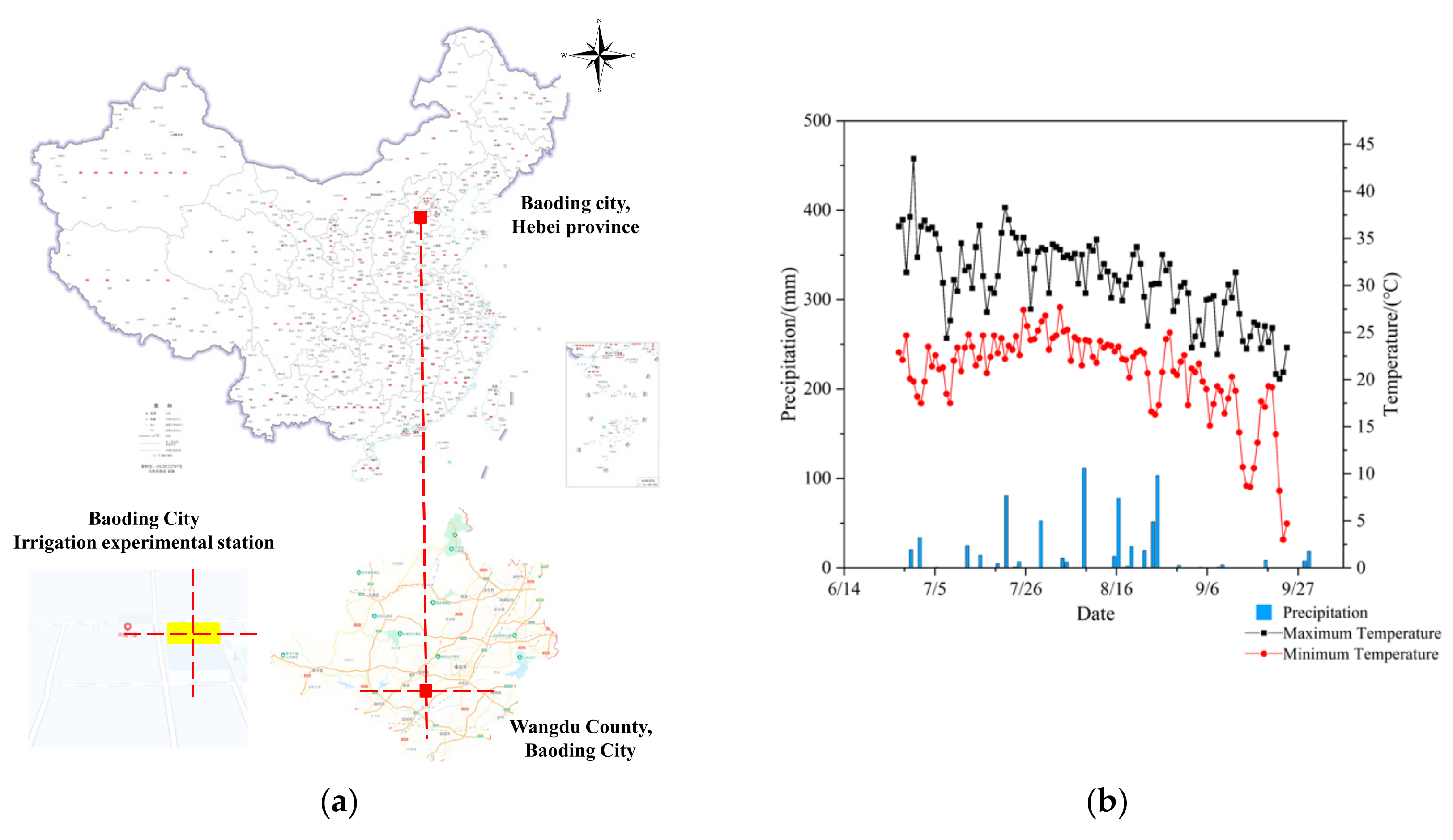
2.1. Study Site and Growth Conditions

The experiment was conducted from June to November 2024 at the Irrigation Experiment Station in Wangdu County, Baoding City, Hebei Province (38°42′ N, 115°6′ E, and elevation 51.0 m above sea level). Figure 1a is the location of geographic position. The region has a temperate semi-arid monsoon climate, with a multi-year average frost-free period of 216.6 days, a multi-year average temperature of 12.5 °C, a multi-year average precipitation of 495.4 mm, a multi-year average sunshine duration of 2316.8 h, and an annual effective accumulated temperature above 10 of 3510 °C. The distribution of local meteorological data is shown in Figure 1b.

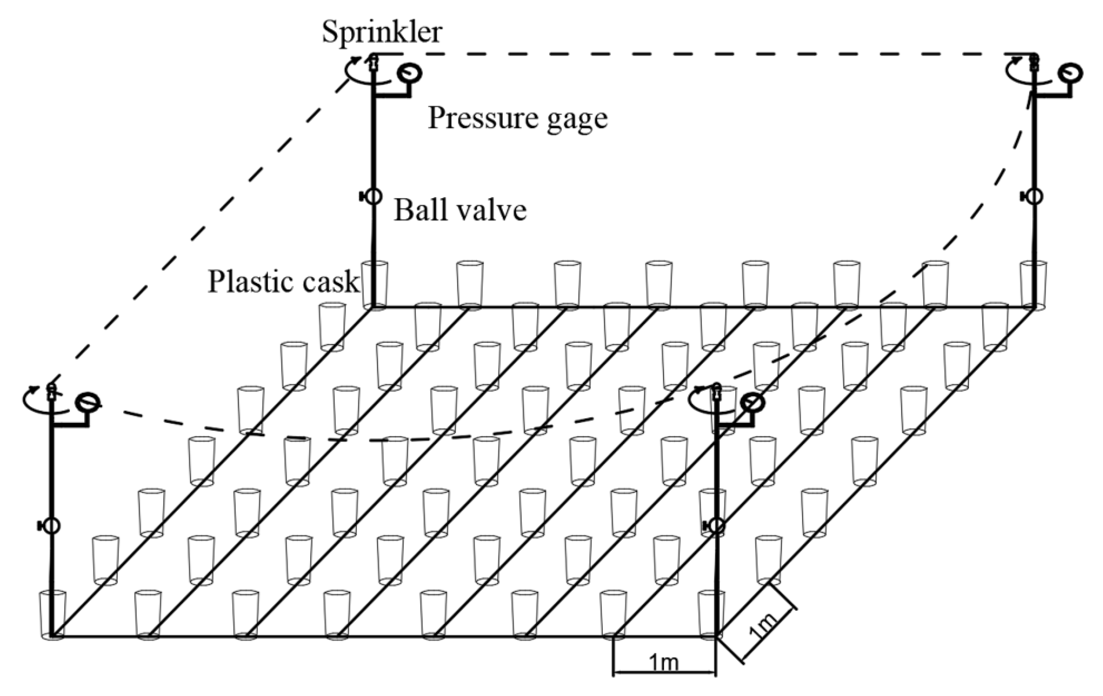
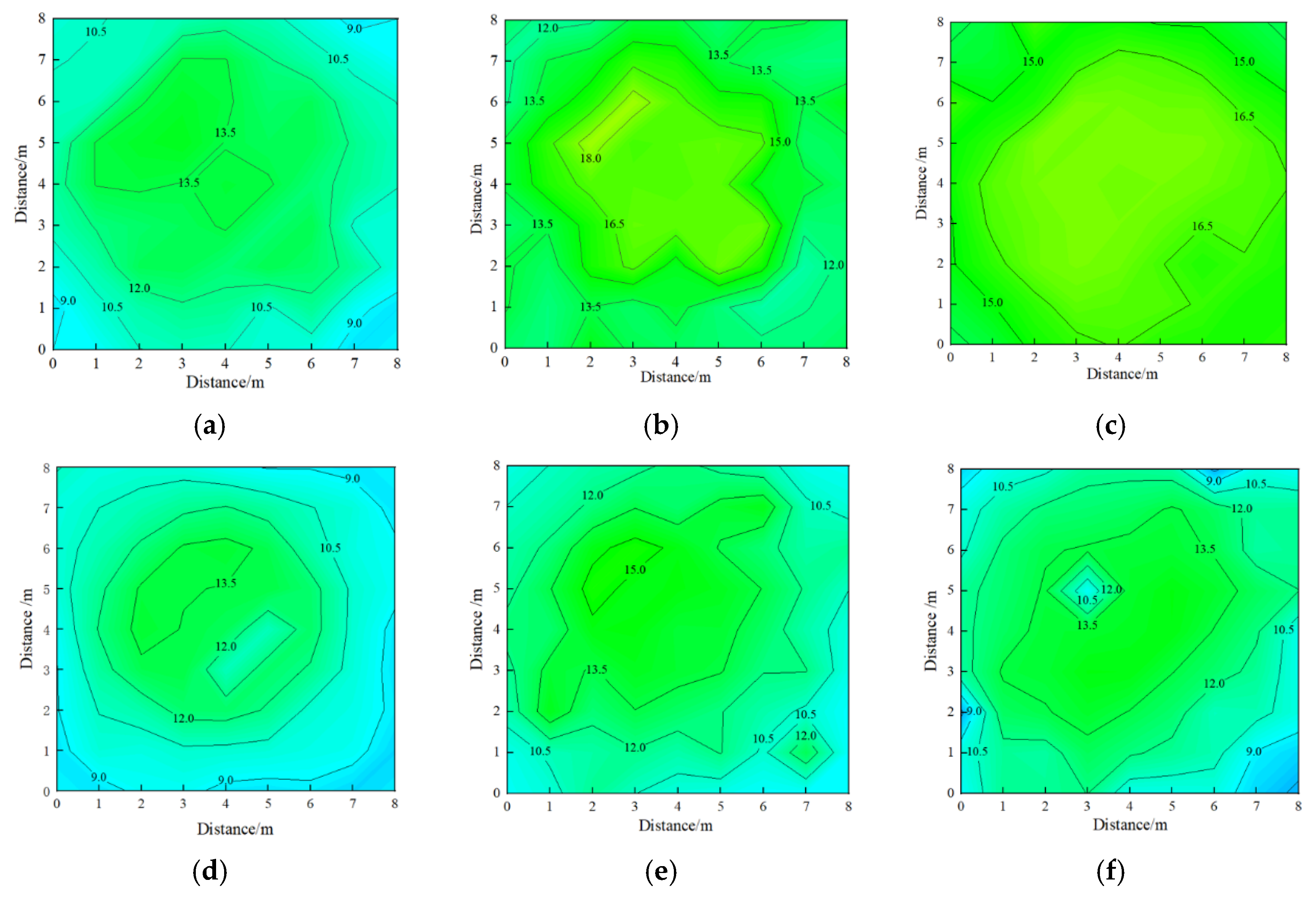
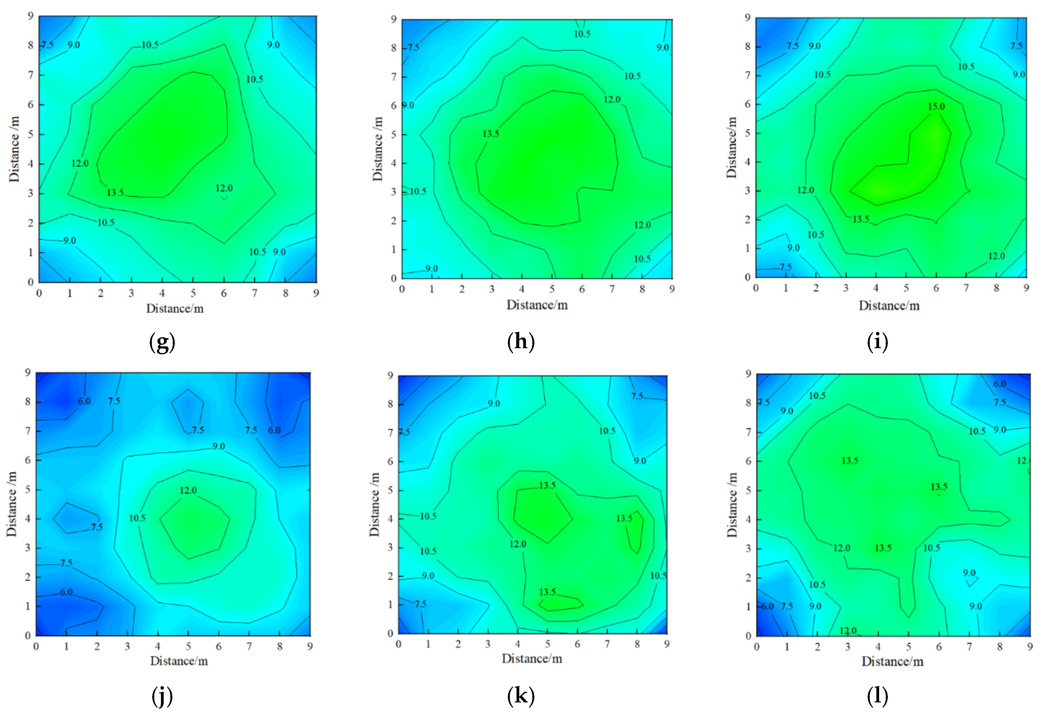
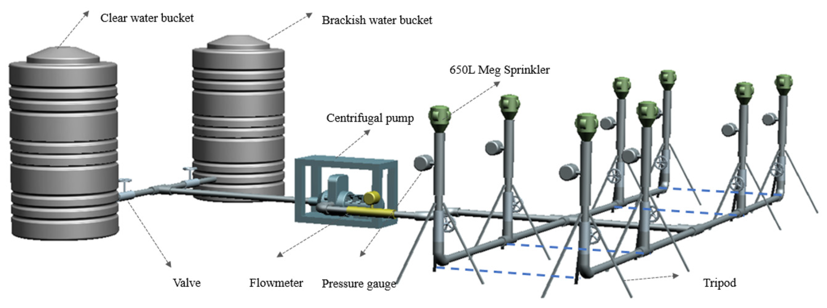
2.2. Water Application Uniformity Test

The corn variety used in the experiment was the commonly used local variety “Ke’en 702.” The sowing date was 19 June 2024, and the harvesting date was 3 October 2024. A water application uniformity test was carried out in 25–27 June 2024. The row spacing of corn was 60 cm, and the plant spacing was 25 cm. The soil in the experimental area was a light loamy cambic Luvisol. The initial average soil water content in the 0–60 cm layer of the experimental area was measured to be 20.84% based on mass. This was determined using the oven-drying method, where fresh soil samples were weighed, dried at 105 °C to a constant weight, and reweighed to calculate water loss. The formula used is provided in Section 2.4. The initial averages of EC, Na⁺ content, Ca²⁺ content, and Mg²⁺ content in the 0–40 cm soil layer were 0.148 mS·cm⁻¹, 16.71 mg·kg⁻¹, 72.35 mg·kg⁻¹, and 15.97 mg·kg⁻¹, respectively.

The experimental procedures and methods for the field combined sprinkler irrigation experiment referred to GB/T 19795.2-2005 “Uniformity of Water Distribution and Test Methods” [24] and the national standard GB/T 22999—2008 “Rotary Nozzles” [25]. The experimental water source comes from local groundwater. The experimental nozzle was a 650 L Meg nozzle, with a range of 8 m and a working pressure of 200–300 kPa. To ensure optimal irrigation performance and system efficiency under different environmental and operational conditions, the experiment selected a combined sprinkler spacing of 1.0 (8 m), 1.1 (8.8 m), 1.2 (9.6 m), and 1.3 R (10.4 m) for comparison (where R is the nozzle range). The working pressure was selected as 200, 250, and 300 kPa. The experimental equipment mainly included a flowmeter, pressure gauge, centrifugal pump, Meg nozzle, ball valve, plastic bucket, and ruler, etc. The nozzles were arranged in a square pattern, with two lateral pipes laid parallel in the north–south direction. Each lateral pipe was equipped with two 650 L Meg nozzles to maximize the coverage area of the nozzles while achieving uniform coverage. The installation height was 1.2 m. The nozzles performed full-circle spraying under different working conditions. Plastic pots for measurement were placed at intervals of 1 m in the experimental area, with the layout of measuring points shown in Figure 2. Since the duration of each experiment was short and water evaporation was minimal, the amount of water in each plastic pot could be considered as the actual irrigation amount [26]. The experiment began after a stable operation of 10 min, with a test duration of 30 min. The amount of water collected in each plastic pot was recorded, and the average value was taken after measurements were repeated 3 times.

The uniformity coefficient of sprinkler irrigation refers to the degree of uniformity in the distribution of water over the irrigated area. In this study, the Christiansen uniformity coefficient was used as the evaluation index [27,28]:

$$C_u=\left[1-{\displaystyle \frac{\sum \left|x_i\right.-\left.x_m\right|}{\sum x_i}}\right]\times 100\%$$

(1)

where $C_u$ is the Christiansen uniformity coefficient, %; $x_i$ is the sprinkled water depth at the i measuring point, mm; and $x_m$ is the average water depth of all measuring points, mm.

During the test, the ambient air temperature ranged from 20.9 to 34.4 °C, the relative humidity ranged from 48.5 to 82.0%, and the wind speed ranged from 0 to 1.51 m·s⁻¹. Figure 3 shows the isohyetal maps of measured sprinkling depths for the 650 L Meg nozzle under experimental working pressures of 200, 250, and 300 kPa, with sprinkler irrigation combination spacings of 1.0, 1.1, 1.2, and 1.3 R during the clear water spraying tests. At 200 kPa, the spraying range is relatively small, with water concentrated near the nozzle, resulting in a limited coverage area. The precipitation is concentrated in the core area, while the outer regions have sparse precipitation, which can easily lead to insufficient coverage. As the pressure increases to 250 kPa, the spraying range significantly expands, increasing the coverage area and distributing the water over a broader region, with the isohyets becoming more evenly spaced. At 300 kPa, the spraying range reaches its maximum, covering a greater distance, with the isohyets extending to the edges of the chart and becoming more densely distributed, presenting a more regular gradient of water depth. Under the same pressure conditions, the effect of different sprinkler irrigation combination spacings on the spraying performance is significant. At a spacing of 1.0 R, the isohyets are relatively evenly distributed, avoiding issues of excessive water overlap or insufficient coverage. At spacings of 1.1 and 1.2 R, the edges of the isohyets begin to show gradual water deficits. At a spacing of 1.3 R, the isohyets are sparsely distributed, with severe water shortages in the edge regions, resulting in significant non-uniformity in the precipitation depth.

The combined uniformity coefficients under different working conditions are shown in

Table 1. Combination uniformity coefficients under different working conditions.

Resultant Nozzle Range/(m)	Working Pressure/(kPa)
	200	250	300
1 R	0.875	0.880	0.932
1.1 R	0.865	0.870	0.859
1.2 R	0.839	0.847	0.835
1.3 R	0.809	0.820	0.811

. As the working pressure increases, the uniformity of combined sprinkler irrigation shows different trends at different combination spacings. When the combination spacing is 1.0 R, the uniformity of combined sprinkler irrigation increases with the increase in working pressure. The uniformity of combined sprinkler irrigation at a working pressure of 300 kPa is 6.51 and 5.91% higher than that at 200 and 250 kPa, respectively. When the combination spacing is 1.1, 1.2, and 1.3 R, the uniformity of combined sprinkler irrigation first increases and then decreases with the increase in working pressure. Under the same working pressure, the uniformity of combined sprinkler irrigation decreases as the combination spacing increases. Under the field experimental conditions, the optimal working pressures for clear water sprinkler irrigation at combination spacings of 1.0, 1.1, 1.2, and 1.3 R are 300, 250, 250, and 250 kPa, respectively. Under the field experimental conditions, the optimal combination spacing for clear water sprinkler irrigation at working pressures of 200, 250, and 300 kPa is 1.0 R. In summary, the optimal working pressure for clear water sprinkler irrigation is 300 kPa, and the optimal combination spacing is 1.0 R (8 m).

2.3. Treatments and Experimental Conditions

The experiments were repeated within a short time interval and in adjacent plots to minimize the differences in initial experimental conditions caused by the physical structural properties of the soil and the spatial heterogeneity of soil water and salt dynamics [29]. The physical properties (such as density and viscosity) of low-saline water and fresh water are different, but under sprinkler irrigation conditions, these differences have little or even negligible impact on the performance of the nozzles. Therefore, the working pressure selected for the saline–freshwater sprinkler irrigation experiment in this study was 300 kPa, with the nozzles arranged in a square pattern and a combination spacing of 8 m.

The saline–freshwater sprinkler irrigation was conducted during the jointing stage of corn. Since the formation of shallow groundwater salinity is the result of both continental salinization and seawater intrusion, and the contents of Na⁺ and Cl⁻ are the highest in saline water, in this experiment, saline water with salinities of 3 and 5 g·L⁻¹ was prepared by adding sea salt to deep groundwater [30]. All irrigation treatments were applied during the corn jointing stage, following a consistent schedule across all plots. The combinations of saline and fresh water were delivered in fixed proportions within each irrigation event and were not adjusted based on the crop growth stage, and the fresh water used in this experiment was deep groundwater. Saline water was prepared by dissolving sea salt into the same groundwater to achieve salinity levels of 3 and 5 g·L⁻¹ for the respective treatments. The experimental field was set up with six treatments. Each treatment had three replicates, resulting in a total of 18 plots, which were randomly arranged. The specific design is shown in

Table 2. Design of experiments.

Treatments	Irrigation Capacity	Treatments Number
3 g·L−1 salty–fresh salty–fresh alternation	1/4 salt water + 1/4 fresh water + 1/4 salt water +1/4 fresh water	S1F1
3 g·L−1 salty–fresh alternation	1/2 salt water + 1/2 fresh water	S1F2
3 g·L−1 salty–fresh mixture	1/2 salt water, 1/2 freshwater mixture	S1F3
5 g·L−1 salty–fresh salty–fresh alternate	1/4 salt water + 1/4 fresh water + 1/4 salt water + 1/4 fresh water	S2F1
5 g·L−1 salty–fresh alternation	1/2 salt water + 1/2 fresh water	S2F2
5 g·L−1 salty–fresh mixture	1/2 salt water, 1/2 freshwater mixture	S2F3

.

Each plot had two lateral pipes laid in the north–south direction, with two nozzles on each pipe, and the plot size was 8 m × 8 m. Each group of field experiments was 64 m long in the east–west direction and 46 m wide in the north–south direction, forming a rectangle, with a total of three groups, as shown in Figure 4. To facilitate the comparative analysis of the experimental results, the irrigation amount was kept consistent across all plots, with an irrigation depth of 62.5 mm, and soil sampling and analysis were conducted before and after irrigation [31].

2.4. Soil Sample Collection

The soil water content was determined using the oven-drying method. Before and after the sprinkler irrigation, soil samples were collected from different soil depths (0–10, 10–20, 20–30, 30–40, 40–50, and 50–60 cm) using the five-point method [32]. The samples were mixed, and then an appropriate amount of soil was taken using the quartering method and placed into bags for subsequent analysis [33]. The fresh soil collected was placed into aluminum soil boxes, labeled, sealed, and brought back to the laboratory. The soil samples were dried in an oven at 105 °C. The calculation formula is as follows [34]:

$$\omega ={\displaystyle \frac{{\omega }_2-{\omega }_3}{{\omega }_3-{\omega }_1}}\times 100\%,$$

(2)

where $\omega$ is the soil water content based on mass, %; ${\omega }_1$ is the mass of the aluminum box, g; ${\omega }_2$ is the mass of the soil sample and aluminum box, g; and ${\omega }_3$ is the mass of the dried soil sample and aluminum box, g.

The soil from 0 to 40 cm was air-dried, ground, and sieved to remove impurities. A soil suspension was prepared at a mass ratio of 5:1 (deionized water to soil sample) and agitated for 3 min using a shaker [35]. The suspension was then filtered immediately. The contents of Na⁺, Ca²⁺, and Mg²⁺ were determined using an Inductively Coupled Plasma Optical Emission Spectrometer (ICAP7400, Thermo Fisher Scientific, Waltham, MA, USA) [36]. The soil EC was measured using a portable multiparameter analyzer (DZB-712, Shanghai INESA, Shanghai, China) [37,38].

2.5. Evaluations on Corn Plants

The corn plant height is defined as the vertical distance from the top of the plant’s aerial growth to the soil surface. During the jointing, tasseling, grain-filling, and maturity stages of corn, three representative plants with consistent growth were randomly selected from each plot. Plant height was measured using a tower ruler with an accuracy of 1 mm. Leaf area was determined for individual leaves based on their geometric dimensions and calculated using Equation (3), which estimates leaf area (LA) in cm². For each selected plant, multiple representative leaves were measured, and the results were averaged [38].

$$\mathrm{L}\mathrm{A}=L\times W\times 0.75,$$

(3)

where LA is the leaf area, cm²; L is the length of the longest part of the leaf, cm; and W is the width of the widest part of the leaf, cm. Both dimensions were measured using a ruler with millimeter precision. The multiplication factor of 0.75 accounts for the elliptical shape of corn leaves.

Before corn harvest, three typical plants were selected from each plot and cut at ground level. The shoot (stems and leaves) was separated from the ears and placed into envelope-style kraft paper bags. The samples were initially killed green in an oven at 105 °C for 2 h, followed by drying at 75 °C until a constant weight was achieved [39]. The dry matter mass of the shoot and the grain yield were then weighed and recorded. The dry matter and grain samples were ground and sieved, and the total nitrogen content was determined using a Kjeldahl nitrogen analyzer (Kiektec2300, Foss, Hillerød, Denmark) [40].

For corn yield estimation, a random sample of corn plants was selected from each plot for yield measurement, and the yield was calculated using a conversion factor of 0.85. Ear length was measured with a ruler, and ear diameter was measured with a caliper. The number of rows and grains per row were counted, and the total weight and weight of 100 grains were weighted after threshing and drying [41].

2.6. Data Analysis

Statistical analysis was conducted using SPSS Statistics 25. One-way ANOVA was employed to test the significant differences among the six treatments. When the significance level was set at p < 0.05, the Least Significant Difference (LSD) test was used to determine the significant differences between different treatments. Data visualization was performed using Origin 2021. The experimental device was modeled with UG NX 12.0, and the schematic diagram of the measuring point arrangement was drawn using CAD 2022.

3. Results and Discussion

As indicated in 2.2., for water application uniformity test, the combination of a working pressure of 300 kPa and a spacing of 1.0 R provides the optimal irrigation uniformity, ensuring a uniform water distribution in the experimental plot, which is crucial for effective water and salt management in brackish water irrigation systems. This optimal configuration was adopted for the saline–freshwater sprinkler irrigation experiments to maximize irrigation efficiency and minimize water deficits at the plot edges.

3.1. Effects of Alternate Salty–Freshwater Irrigation on Soil Water Distribution

The effects of different sprinkler irrigation modes and low-saline water salinity levels (3 and 5 g·L⁻¹) on soil water content across six soil depths (0–10, 10–20, 20–30, 30–40, 40–50, and 50–60 cm) are presented in

Table 3. Mass-based soil moisture content (%) at different soil depths under each treatment.

Treatments	Soil Depth (cm)
	0–10	10–20	20–30	30–40	40–50	50–60
S1F1	0.221 a	0.208 a	0.204 a	0.206 a	0.202 a	0.203 a
S1F2	0.219 a	0.209 a	0.201 ab	0.202 b	0.201 a	0.202 a
S1F3	0.213 b	0.202 b	0.198 b	0.196 cd	0.195 b	0.199 b
S2F1	0.209 c	0.200 c	0.199 b	0.195 cd	0.195 b	0.199 b
S2F2	0.207 c	0.201 c	0.198 b	0.194 d	0.194 b	0.198 b
S2F3	0.210 c	0.201 c	0.199 b	0.198 c	0.196 b	0.199 b

Note: In the table, S1F1, S1F2, S1F3, S2F1, S2F2, and S2F3 are, respectively, 3 g·L⁻¹ salty–fresh salty–fresh alternation, 3 g·L⁻¹ salty–fresh alternation, 3 g·L⁻¹ salty–fresh mixture, 5 g·L⁻¹ salty–fresh salty–fresh alternate, 5 g·L⁻¹ salty–fresh alternation, and 5 g·L⁻¹ salty–fresh mixture. Values followed by different lowercase letters within the same soil depth are significantly different at p < 0.05. Statistical differences were determined using one-way ANOVA followed by LSD post hoc test.

. Overall, the 3 g·L⁻¹ salinity treatments (S1F1, S1F2, and S1F3) generally maintained a higher soil water content than the 5 g·L⁻¹ treatments (S2F1, S2F2, and S2F3) across all depths, particularly in the deeper layers (30–60 cm). This is attributed to the lower Na⁺ content in 3 g·L⁻¹ low-saline water, which causes less disruption to the soil structure compared to 5 g·L⁻¹ water. The higher Na⁺ in 5 g·L⁻¹ treatments (S2F1, S2F2, and S2F3) likely displaced Ca²⁺ in soil colloids, reducing soil cohesion and increasing aeration pores, which facilitated greater water loss due to gravitational forces. Among the 3 g·L⁻¹ treatments, S1F1 (saline–fresh–saline–fresh alternating) consistently showed the highest water content, particularly in deeper layers, due to its effective leaching of salts and maintenance of soil pore stability through periodic freshwater irrigation [42]. S1F2 (saline–fresh alternating) performed similarly to S1F1 in most layers, indicating that both alternating modes are effective at promoting water retention. In contrast, S1F3 (mixed saline–fresh) had a lower water content, likely due to less effective salt leaching. For the 5 g·L⁻¹ treatments, S2F1 showed a slightly better water retention than S2F2 and S2F3 in the deeper layers, suggesting that the saline–fresh–saline–fresh alternating mode mitigates some of the negative effects of higher salinity. However, S2F2 and S2F3 exhibited similar water content profiles, indicating that the saline–fresh alternating and mixed modes have comparable limitations under high salinity conditions.

The experimental site’s temperate semi-arid monsoon climate, characterized by high evaporation rates, further influenced surface soil moisture dynamics [39]. Alternating sprinkler irrigation modes (S1F1, S1F2, S2F1, and S2F2) reduced evaporation losses by increasing irrigation frequency and reducing single irrigation volumes, promoting uniform water infiltration. The mixed irrigation mode (S1F3, S2F3), however, showed less pronounced benefits, particularly at 3 g·L⁻¹, due to continuous salt input without sufficient leaching. These findings highlight the superiority of alternating saline–fresh irrigation, especially S1F1, in optimizing the soil water distribution by stabilizing soil structure, suppressing surface evaporation, and promoting deepwater migration, with the 3 g·L⁻¹ salinity level being more effective than 5 g·L⁻¹.

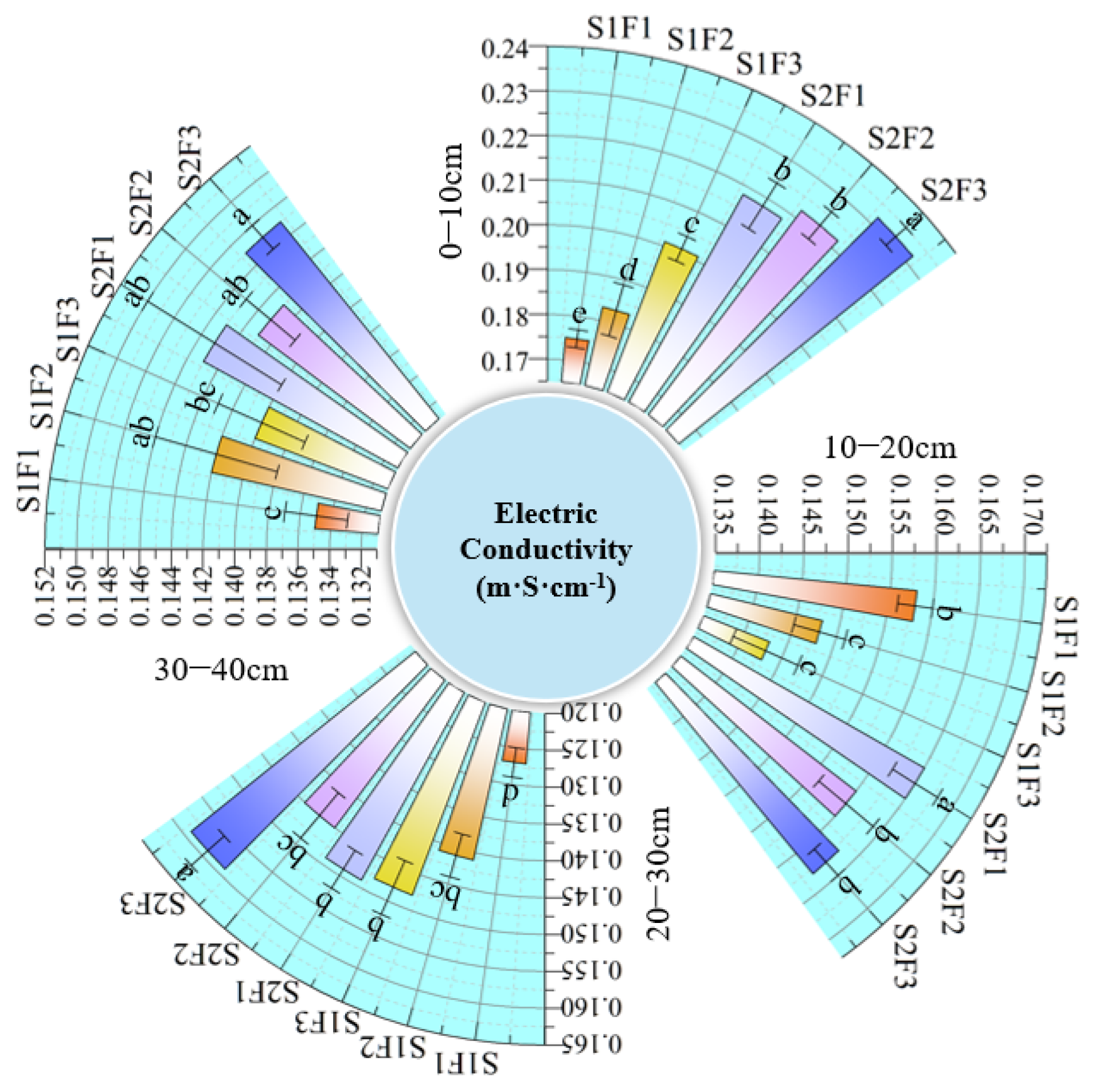
3.2. Effects of Alternate Salty–Freshwater Irrigation on Soil Electrical Conductivity

EC can intuitively reflect the salt content in the soil. The effects of different sprinkler irrigation modes and low-saline water salinity on soil water content is shown in Figure 5. Under different irrigation methods, the EC values of the soil irrigated with low-saline water in S1F1, S1F2, and S1F3 first decreased and then increased. In contrast, the EC values in S2F1, S2F2, and S2F3 decreased with increasing soil depth, which is related to the dynamic process of soil water infiltration and salt migration [43]. In the soil profile, the inflection points of EC values for S1F1 and S1F2 were located at the 30–40 cm soil layer, while for S1F3, the inflection point was at the 20–30 cm soil layer. Compared with S1F3, the EC values of S1F1 and S1F2 decreased by 18.54 and 6.62%, respectively. The different inflection points of the soil EC values with increasing soil depth are due to the following reasons: in alternating sprinkler irrigation, when low-saline water is first applied, the EC value in the soil surface layer increases rapidly. Subsequently, when fresh water is sprinklered, the soil salinity and soil matrix potential change, and the fresh water carries the salt from the surface layer to deeper layers, reducing the salt content in the surface soil. The alternating saline–fresh sprinkler irrigation moves the surface salts down to the 30–40 cm soil layer. Under the same irrigation mode, for low-saline water with salinities of 3 and 5 g·L⁻¹, the higher the salinity of the low-saline water, the higher the EC value at the same soil depth.

The vertical variation in EC values reflects the interplay between irrigation sequencing and salt redistribution. The clear inflection points at 30–40 cm for S1F1 and S1F2 indicates that freshwater pulses facilitated salt leaching to deeper zones, effectively reducing surface EC levels. In contrast, the higher surface EC under S1F3 highlights the limitations of mixing, where insufficient salt displacement leads to surface accumulation. Importantly, the decline in EC with depth under high-salinity treatments (S2 group) suggests gravitational and matric-driven salt migration, though the increased osmotic pressure likely impedes further downward leaching. These findings suggest that alternating irrigation not only affects the EC’s magnitude but also its spatial distribution, with potential implications for long-term salt stratification and root-zone management.

3.3. Effects of Alternate Salty–Freshwater Sprinkler Irrigation on Na⁺, Mg^{2 +}, and Ca^{2 +} Content

Na⁺ content in soil is an important indicator of soil salinity and directly affects soil pore structure and crop growth [44]. The changes in Na⁺ content with soil depth for each treatment are shown in

Table 4. The contents of Na⁺, Mg²⁺, and Ca²⁺ in different soil depths were measured.

Treatments	Na+ (mg·kg−1)				Mg2+ (mg·kg−1)				Ca2+ (mg·kg−1)
	Soil Depth (cm)				Soil Depth (cm)				Soil Depth (cm)
	0–10	10–20	20–30	30–40	0–10	10–20	20–30	30–40	0–10	10–20	20–30	30–40
S1F1	40.973 f	18.160 e	17.135 e	20.065 b	10.394 d	9.967 e	9.149 d	9.481 d	67.172 e	66.541 e	64.793 e	71.759 e
S1F2	41.934 e	18.889 e	18.180 d	18.149 de	14.461 b	11.695 d	13.109 b	14.346 a	68.647 d	70.610 d	73.401 d	79.108 d
S1F3	43.644 d	25.151 d	18.851 c	17.519 e	14.664 b	15.968 b	14.873 a	14.648 a	69.005 d	70.450 d	74.389 c	79.108 cd
S2F1	51.741 c	30.952 c	18.990 c	22.557 a	12.029 c	10.133 e	11.248 c	10.926 c	79.813 c	83.542 c	79.139 b	79.742 bc
S2F2	53.600 b	35.239 b	22.475 b	19.312 c	15.008 b	14.908 c	12.839 b	13.337 b	81.307 b	84.667 b	79.322 b	81.670 a
S2F3	57.760 a	38.576 a	23.757 a	18.465 d	17.062 a	16.722 a	15.138 a	14.797 a	83.203 a	88.396 a	85.422 a	80.212 b

Note: In the table, S1F1, S1F2, S1F3, S2F1, S2F2, and S2F3 are, respectively, 3g·L⁻¹ salty–fresh salty–fresh alternation, 3 g·L⁻¹ salty–fresh alternation, 3 g·L⁻¹ salty–fresh mixture, 5 g·L⁻¹ salty–fresh salty–fresh alternate, 5 g·L⁻¹ salty–fresh alternation, and 5 g·L⁻¹ salty–fresh mixture. Values followed by different lowercase letters within the same soil depth are significantly different at p < 0.05, as determined by one-way ANOVA followed by LSD post hoc test.

. The results of a variance analysis indicate that significant differences in Na⁺ content are evident with an increasing treatment concentration and depth. The S1F1 treatment exhibited lower Na⁺ content in the surface layer (0–10 cm), with significant differences compared to other treatments (p < 0.05), while S2F3 reached the highest level at the same depth. The Na⁺ content in S1F1 and S2F1 treatments first decreased and then increased with soil depth, with the inflection point located at the 30–40 cm soil layer. Compared with S1F1, the Na⁺ content in S1F2 and S1F3 at this depth decreased by 9.55 and 12.69%, respectively. Compared with S2F1, the Na⁺ content in S2F2 and S2F3 decreased by 14.39 and 18.14%, respectively. Under the same irrigation method, for low-saline water with salinities of 3 and 5 g·L⁻¹, the higher the salinity, the higher the Na⁺ content at the same soil depth.

Mg²⁺ content in soil is one of the important indicators for assessing soil fertility and is an essential nutrient for plant growth [42]. Significant differences in Mg²⁺ content were observed among different soil layers under various sprinkler irrigation modes, especially in the 0–10 cm soil layer, with Mg²⁺ content decreasing with increasing soil depth. The S1F1 and S2F1 treatments maintained lower Mg²⁺ content in the 0–40 cm soil layer. The 3 g·L⁻¹ low-saline water was more conducive to the vertical uniform distribution of Mg²⁺, while the 5 g·L⁻¹ low-saline water mixed treatment promoted the accumulation of Mg²⁺, particularly in the surface and middle soil layers.

Ca²⁺ is an important indicator of soil quality and plays a significant role in maintaining soil structure stability and enhancing the soil cation exchange capacity (CEC) [45]. The content of Ca²⁺ was higher in the surface layer and gradually decreased with increasing soil depth. The S2F3 treatment exhibited significantly higher Ca²⁺ content in the 0–10 cm soil layer (p < 0.05), while differences among treatments were smaller in the 30–40 cm soil layer. The average Ca²⁺ content in the 0–40 cm soil layer for different treatments is shown in

Table 5. Effects of each treatment on corn yield related indexes.

Treatments	Spike Diameter (cm)	Spike Length (cm)	100-Seed Weight (g)	Grain Number Per Spike (n)	Output (kg·hm−2)
S1F1	5.49 ± 0.02 a	22.66 ± 0.31 a	32.63 ± 0.81 a	640 ± 12 a	9305.90 ± 50.25 a
S1F2	5.45 ± 0.02 a	22.68 ± 0.15 a	31.95 ± 0.78 ab	626 ± 8 a	9165.49 ± 49.93 b
S1F3	5.36 ± 0.26 b	22.46 ± 0.11 ab	31.49 ± 0.53 bc	628 ± 11 ab	9106.67 ± 29.79 bc
S2F1	5.32 ± 0.17 bc	22.24 ± 0.10 b	30.83 ± 0.09 cd	606 ± 9 bc	9023.92 ± 42.62 cd
S2F2	5.33 ± 0.25 bc	22.16 ± 0.10 bc	30.90 ± 0.87 cd	583 + 12 cd	9044.31 ± 37.82 cd
S2F3	5.29 ± 0.02 c	21.95 ± 0.15 c	30.39 ± 0.21 d	589 ± 17 d	9005.49 ± 44.59 d

Note: In the table, S1F1, S1F2, S1F3, S2F1, S2F2, and S2F3 are, respectively, 3 g·L⁻¹ salty–fresh salty–fresh alternation, 3 g·L⁻¹ salty–fresh alternation, 3 g·L⁻¹ salty–fresh mixture, 5 g·L⁻¹ salty–fresh salty–fresh alternate, 5 g·L⁻¹ salty–fresh alternation, and 5 g·L⁻¹ salty–fresh mixture. Values followed by different lowercase letters within the same column are significantly different at p < 0.05, based on one-way ANOVA followed by LSD post hoc test.

. The initial Ca²⁺ content in the 0–40 cm soil was 72.35 mg·kg⁻¹. Compared with the initial soil, the average content of Ca²⁺ in S1F1, S1F2, and S1F3 decreased by 20.92, 23.78, and 32.16%, respectively. In contrast, S2F1, S2F2, and S2F3 increased the average Ca²⁺ content by 16.90, 20.13, and 10.95%, respectively. Moreover, the higher the salinity of the low-saline water, the higher the Ca²⁺ content at the same soil depth. Ion exchange between Na⁺ in low-saline water and Ca²⁺ in the soil led to changes in Ca²⁺ content, and higher salinity water promoted the release of more Ca²⁺ from soil colloids [46]. Guo et al. [43] found that the effects triggered by saline water irrigation significantly increased the ionic strength of the soil solution, raising the risk of salt ion hazards, which is consistent with the higher Na⁺, Mg²⁺, and Ca²⁺ contents observed in the soil treated with 5 g·L⁻¹ low-saline water in this study. The changes in osmotic pressure caused by high-concentration saline water significantly affected ion exchange processes, leading to an increased salt ion accumulation in the soil. Different sprinkler irrigation methods of low-saline water result in significantly different behaviors in the soil. The salt ions brought into the soil by low-saline water mainly accumulate in the surface soil layer. Compared with continuous saline–freshwater (SF) irrigation, alternating irrigation helps to migrate salts from the surface soil to deeper layers, creating a leaching effect, especially for the S1F1 irrigation mode, which showed a more significant leaching effect on soil salts.

The different ion responses across treatments reflect both ion mobility and exchange reactions. Lower surface Na⁺ and Mg²⁺ under S1F1 imply that freshwater cycles interrupted salt accumulation and facilitated cation displacement and downward leaching. The stable Mg²⁺ profile in S1F1 also indicates less interference with soil colloidal stability, which is critical for maintaining structure and aeration. In contrast, S2F3 led to the notable surface accumulation of all ions, driven by repeated saline inputs and a lack of leaching pulses. The significant reduction in Ca²⁺ under S1F1 suggests cation exchange processes where Na⁺ displaces Ca²⁺, but alternation mitigates its impact. These patterns highlight that irrigation mode—not just salinity—determines ion migration, with consequences for soil fertility, cation exchange capacity (CEC), and plant ion uptake.

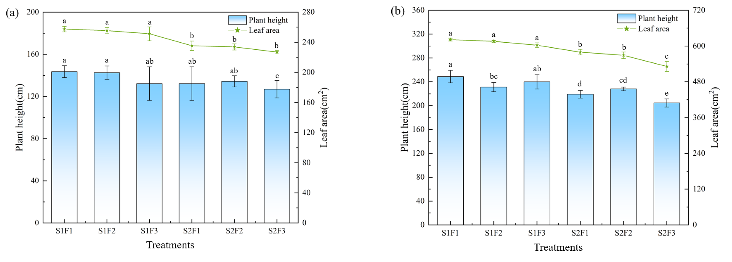
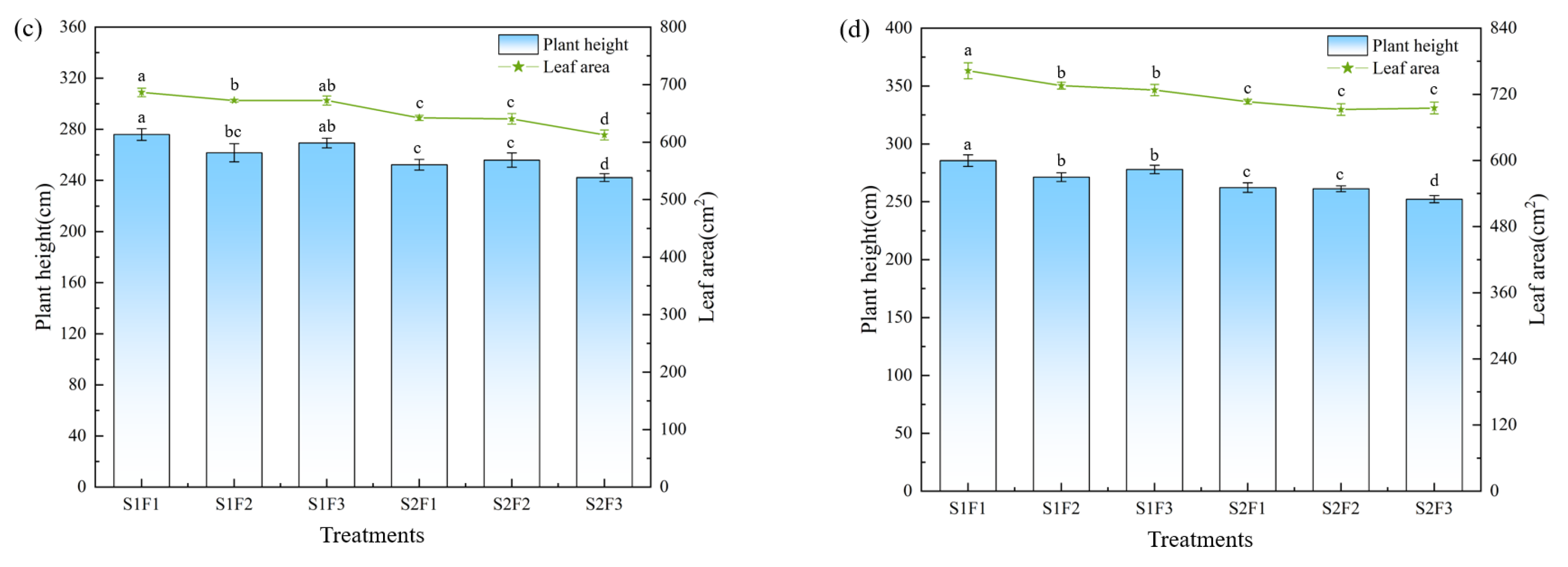
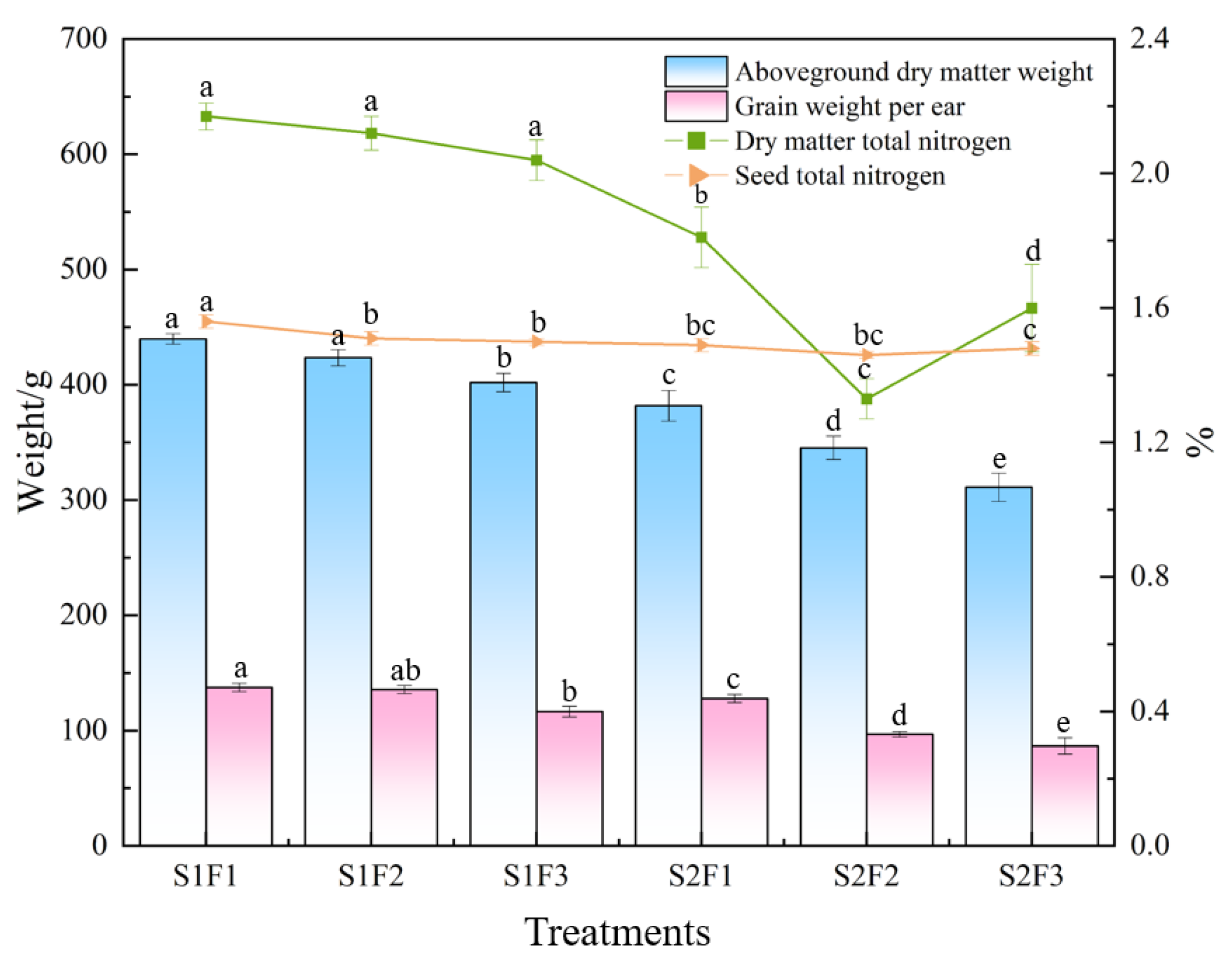
3.4. Effects of Alternate Salty–Freshwater Sprinkler Irrigation on Corn Growth

The effects of different treatments on corn plant height and leaf area during the jointing, tasseling, grain-filling, and maturity stages are shown in Figure 6. Corn plant height and leaf area increased continuously with the developmental stages, and the effects were significantly influenced by the salinity concentration and treatment methods. Statistical analysis showed that at each developmental stage, S1F1 had a significantly higher plant height and leaf area compared to S1F3 (p < 0.05). At maturity, the plant height of S1F1 was 2.7% higher than S1F3, which was statistically significant. Similarly, S2F1 was significantly better than S2F3 under 5 g·L⁻¹ conditions (p < 0.05). Under the same salinity concentration, alternating saline–fresh treatments (F1/F2) generally performed better than the mixed treatment (F3). At 3 g·L⁻¹ salinity, during the jointing stage, the plant height of S1F1 was 8.6% higher and the leaf area was 3.0% higher than those of S1F3. At maturity, the plant height and leaf area of S1F1 were 2.7 and 2.6% higher, respectively. At 5 g·L⁻¹ salinity, the plant height of S2F1 at maturity was 3.9% higher, and the leaf area was 0.66% higher than those of S2F3. The differences among treatments gradually narrowed after the tasseling stage. Overall, the plant height and leaf area of the 3 g·L⁻¹ treatments were higher than those of the 5 g·L⁻¹ treatments. Under low salinity conditions, alternating saline–fresh treatments promoted growth more effectively, while under high salinity stress, alternating treatments still partially alleviated the inhibitory effects. The reason is that under low salinity (3 g·L⁻¹), alternating saline–fresh sprinkler irrigation achieved a virtuous cycle of “salt dilution-leaching-uniform distribution,” meeting the crop’s water needs while avoiding excessive salt accumulation. Under high salinity (5 g·L⁻¹), even with alternating modes (such as S2F1), the overall salt input was still high, leading to osmotic stress and ion toxicity (e.g., significant increase in Na⁺ content), resulting in lower increases in plant height and leaf area compared to the 3 g·L⁻¹ treatments.

Aboveground dry matter accumulation, grain weight, total nitrogen in dry matter, and total nitrogen in grains are core indicators characterizing the growth and development of crops and can serve as key parameters for yield prediction and field management decision-making [47]. The effects of different treatments on aboveground dry matter weight, grain weight, total nitrogen in dry matter, and total nitrogen in grains of summer corn are shown in Figure 7. The results indicate that with the increasing salinity of irrigation water, corn’s aboveground dry matter weight, total nitrogen content in dry matter, grain yield, and total nitrogen content in grains all significantly decreased (p < 0.05), with S2F3 being the most unfavorable. Under the same salinity level, F1 was superior to other treatments in promoting dry matter accumulation and nitrogen uptake, with S1F1 showing the best performance and significantly increasing corn biomass (p < 0.05). F1 reduced the root-zone salinity concentration through periodic freshwater irrigation, alleviating salt stress, while F3 exacerbated inhibitory effects due to continuous salt accumulation. A salinity of 5 g·L⁻¹ significantly reduced grain yield (p < 0.05). Within the same salinity group, the order was F1 > F2 > F3. High salinity interfered with the synthesis of carbohydrates and proteins during the grain-filling stage and inhibited the translocation of photosynthetic products to the grains [48]. Although 5 g·L⁻¹ led to a slight decrease in grain nitrogen content, the differences within the S2 group were not significant. Grain nitrogen content is less sensitive to salinity because nitrogen is preferentially allocated to the grains to maintain protein synthesis. Salinity mainly affects nitrogen translocation efficiency rather than the nitrogen metabolic processes within the grains.

The enhanced plant height and leaf area under S1F1 result from improved root-zone moisture availability and reduced salt stress during critical development stages. Alternating irrigation likely created a buffering environment: freshwater intervals minimized osmotic and toxic ion effects, while the saline inputs preserved soil moisture by limiting excessive leaching. The diminishing treatment differences after the tasseling stage suggest that early-stage soil conditions have the most influence on vegetative growth. In contrast, the consistently poor performance of S2F3 reveals how continuous exposure to salinity can suppress physiological growth through ionic imbalance and metabolic disruption. These results suggest that dynamic irrigation scheduling—not just water quality—should be optimized to support early biomass establishment under salinity pressure.

3.5. Effects of Alternate Salty–Freshwater Sprinkler Irrigation on Corn Yield

As shown in Table 5, the ear diameter, number of grains per ear, weight of 100 grains, and yield of the S1F1 treatment were the highest among all treatments. Under the same concentration, compared with S1F3, the ear diameter of S1F1 and S1F2 increased by 2.4% and 1.68%, respectively, the weight of 100 grains increased by 3.6 and 1.4%, respectively, and the yield increased by 2.2 and 0.6%, respectively. Compared with S2F3, the ear diameter of S2F1 and S2F2 increased by 0.6 and 0.7%, respectively, the weight of 100 grains increased by 1.4 and 1.7%, respectively, and the yield increased by 0.2 and 0.4%, respectively. Under the same alternating mode, compared with S2F1, the ear diameter, ear length, weight of 100 grains, number of grains per ear, and yield of S1F1 increased by 3.1, 1.9, 5.8, 5.6, and 3.1%, respectively. Compared with S2F2, the ear diameter, ear length, weight of 100 grains, number of grains per ear, and yield of S1F2 increased by 2.4, 2.3, 3.3, 7.4, and 1.3%, respectively. Compared with S2F3, the ear diameter, ear length, weight of 100 grains, number of grains per ear, and yield of S1F3 increased by 1.3, 2.3, 3.6, 3.6, 6.5, and 1.1%, respectively. At 3 g·L⁻¹, the optimized sprinkler irrigation mode (F1 → F2 → F3) can increase the yield by 1.8%, while at 5 g·L⁻¹, the increase is only 0.4%, indicating that sprinkler irrigation regulation is more effective under low-salinity conditions. The S1F1 treatment performed the best overall, with a yield increase of 3.0% compared to S2F3, and all indicators were significantly higher (p < 0.05). The yields of all 3 g·L⁻¹ treatments were significantly higher than those of the 5 g·L⁻¹ treatments (p < 0.05). When salinity is lower, the osmotic stress on corn roots is reduced, and the efficiency of water and nutrient uptake is higher, which directly improves ear development (ear diameter and number of grains per ear) and grain filling (weight of 100 grains). In summary, salinity concentration is the main limiting factor for the yield, while the sprinkler irrigation mode alleviates the salt stress effect by regulating the water and salt dynamics in the root zone.

Yield differences across treatments are best explained by the cumulative impact of salt stress on reproductive development. S1F1’s superior ear diameter, grain number, and 100-grain weight reflect improved assimilate partitioning and translocation efficiency, which depend on sustained root function and photosynthesis. The alternating saline–fresh regime likely preserved the root membrane integrity and delayed salinity-induced senescence, especially under 3 g·L⁻¹ conditions. In contrast, yield suppression in S2F3 indicates that prolonged ionic toxicity and osmotic stress hampered grain filling, even if vegetative traits appeared similar. Thus, yield response is not merely a reflection of salinity level, but also of the soil’s temporal salt load, which is best managed through alternating irrigation cycles that synchronize with crop phenological needs.

4. Conclusions

This study investigated the effects of alternate saline–freshwater sprinkler irrigation with two salinity levels (3 and 5 g·L⁻¹) and three irrigation strategies (F1, F2, F3) on soil water–salt transport and corn growth. The key conclusions are:

• Soil water–salt regulation: The S1F1 treatment (3 g·L⁻¹, alternate saline–fresh–saline–fresh) significantly improved soil water retention in the 30–50 cm layer and reduced surface salt accumulation (p < 0.05). This mode promoted deeper salt leaching and maintained ion balance, especially for Na⁺ and Mg²⁺.
• Corn growth and yield: S1F1 consistently outperformed other treatments in plant height, leaf area, biomass accumulation, and yield-related traits. Compared to S2F3, S1F1 increased the yield by up to 3.0% and improved the 100-grain weight and grain number per ear.
• Salinity sensitivity: Lower salinity (3 g·L⁻¹) was more favorable for soil structure stability and crop productivity. High salinity (5 g·L⁻¹) aggravated salt stress, particularly under the mixed irrigation mode (F3), leading to a reduced yield and poor ion distribution.
• Practical implication: The S1F1 strategy provides an effective solution for utilizing low-saline water in semi-arid regions, especially in the North China Plain. Its ability to balance water-saving and yield protection supports its application in sustainable agriculture.

Future Work: Further research is recommended to explore the long-term effects of alternate irrigation cycles, irrigation intensity, and water quality combinations on soil health and crop performance.

References

1. GB/T 14157-2023; National Technical Committee for Standardization of Natural Resources and Territorial Spatial Planning (SAC/TC 93). Terminology of Hydrogeology. Standards Press of China: Beijing, China, 2023.
2. Sun, H.; Zhang, X.; Tian, L.; Lou, B.; Liu, T.; Wang, J.; Dong, X.; Guo, K.; Liu, X. Research progress on the effect of saline water irrigation on cultivated land quality and crop production. Chin. J. Ecol. Agric. 2023, 31, 354–363, (In Chinese with English abstract). [Google Scholar]
3. Wang, D.; Kang, Y.; Wang, S. Distribution characteristics of different salt ions in soil under drip irrigation with brackish water. Trans. Chin. Soc. Agric. Eng. 2007, 23, 83–87, (In Chinese with English abstract). [Google Scholar]
4. Guo, L.; Bi, Y.; Ma, J.; Guo, X.; Sun, X.; Wei, L. Study on the effect of alternate drip irrigation on soil water and salt distribution. Conserv. Irrig. 2016, 5, 6–11, (In Chinese with English abstract). [Google Scholar]
5. Rngasamy, P. Soil processes affecting crop production in salt-affected soils. Funct. Plant Biol. 2020, 37, 613–620. [Google Scholar] [CrossRef]
6. Maas, E.V.; Glenn, J.H. Hoffman. Crop salt tolerance—current assessment. J. Irrig. Drain. Div. 1977, 103, 115–134. [Google Scholar] [CrossRef]
7. Ayers, R.S.; Dennis, W.W. Westcot. Water Qual. Agric. 1985, 29, 174. [Google Scholar]
8. IUSS Working Group WRB. World Reference Base for Soil Resources: International Soil Classification System for Naming Soils and Creating Legends for Soil Maps, 4th ed.; International Union of Soil Sciences (IUSS): Vienna, Austria, 2022. [Google Scholar]
9. Bi, W.; Lin, D.; Mao, X. Two-dimensional migration law of soil water, heat and salt and suitable irrigation system of drip irrigation under brackish water film in cotton field of southern Xinjiang. Trans. Chin. Soc. Agric. Eng. 2024, 40, 155–168, (In Chinese with English abstract). [Google Scholar]
10. Karlberg, L.; Rockstrom, J.; Annandale, J.G. Low-cost drip irrigation–a suitable technology for southern Africa: An example with tomatoes using saline irrigation water. Agric. Water Manag. 2007, 89, 59–70. [Google Scholar] [CrossRef]
11. Sheng, F.; Zhang, M.; Xue, R.; Hu, G.; Zhan, H.; Wei, R. Effects of salinity in irrigation water on soil structure and water flow characteristics. J. Hydraul. Eng. 2019, 50, 346–355, (In Chinese with English abstract). [Google Scholar]
12. Yang, G.; Li, F.; Tian, L.; He, X.; Gao, Y.; Wang, Z.; Ren, F. Soil physicochem (Gossypium hirsutum) ical properties and cottonyield under brackish water mulched drip irrigation. Soil Tillage Res. 2020, 199, e104592. [Google Scholar] [CrossRef]
13. He, Y.; Tan, J.; Wang, X.; Dong, H. Effects of different brackish water irrigation methods on spatial variability of soil water, salt and pH in gravel-mulched field. Conserv. Irrig. 2023, 8, 1–9, (In Chinese with English abstract). [Google Scholar]
14. Grieve, C.M.; Wang, D.; Shannon, M.C. Salinity and irrigation method affect mineral ion relations of soybean. J. Plant Nutr. 2003, 26, 901–913. [Google Scholar] [CrossRef]
15. Sun, Z.; Kang, Y.; Jiang, S. Effects of water application intensity, drop size and water application amount on the characteristics of topsoil pores under sprinkler irrigation. Agric. Water Manag. 2008, 95, 869–876. [Google Scholar] [CrossRef]
16. Chu, L.; Kang, Y.; Chen, X.; Li, X. Effects of sprinkler irrigation intensity on soil water and salt transport characteristics in coastal saline-alkali land. Trans. Chin. Soc. Agric. Eng. 2013, 29, 76–82, (In Chinese with English abstract). [Google Scholar]
17. Wang, Y.; Yang, P.; Ren, S.; He, X.; Wei, C.; Wang, S.; Xu, Y.; Xu, Z.; Zhang, Y.; Ismail, H. CO2 and N2O emissions from spring corn soil under alternate irrigation between saline water and groundwater in hetao irrigation district of inner mongolia, China. Int. J. Environ. Res. Public Health 2019, 16, 2669. [Google Scholar] [CrossRef]
18. Sevostianova, E.; Leinauer, B.; Sallenave, R.; Karcher, D.; Maier, B. Soil salinity and quality of sprinkler and drip irrigated cool-season turfgrasses. Agron. J. 2011, 103, 1503–1513. [Google Scholar] [CrossRef]
19. Jiao, Y.; Wang, H.; Zhang, S.; Chen, W.; Zheng, H. Effects of sprinkler irrigation with mixed saline-fresh water on soil water and salt transport and yield of wheat and corn. Agric. Res. Arid. Areas 2021, 39, 87–94, (In Chinese with English abstract). [Google Scholar]
20. Mi, Y.; Qu, M.; Yang, J.; Yu, S. Study on the Effects of saline-fresh water rotation irrigation on soil salinity and crop yield. J. Irrig. Drain. 2010, 29, 83–86, (In Chinese with English abstract). [Google Scholar]
21. Singh, A. Conjunctive use of water resources for sustainable irrigated agriculture. J. Hydrol. 2014, 519, 1688–1697. [Google Scholar] [CrossRef]
22. Singh, R. Simulations on direct and cyclic use of saline waters for sustaining cotton–wheat in a semi-arid area of north-west India. Agric. Water Manag. 2004, 66, 153–162. [Google Scholar] [CrossRef]
23. Huang, J.; Jin, M.; Li, X. Effects of alternative irrigation with brackish and freshwater on cotton yields and solute transport in soil. Trans. Chin. Soc. Agric. Eng. 2015, 31, 99–107, (In Chinese with English abstract). [Google Scholar]
24. GB/T 27612.3—2011; General Administration of Quality Supervision, Inspection and Quarantine of the People’s Republic of China, Standardization Administration of China. Agricultural Irrigation Equipment—Sprinklers—Part 3: Characterization of Distribution and Test Methods. Standards Press of China: Beijing, China, 2012.
25. GB/T 22999—2008S; General Administration of Quality Supervision, Inspection and Quarantine of the People’s Republic of China, Standardization Administration of China. Standards Press of China: Beijing, China, 2009.
26. Jiang, Y.; Wang, L.; Li, H.; Zuo, X. Study on hydraulic performance of rocker-arm sprinkler under the condition of aquaculture fertilizer water sprinkler irrigation. J. Irrig. Drain. 2024, 43, 61–67+85, (In Chinese with English abstract). [Google Scholar]
27. Xue, S.; Ge, M.; Wei, F.; Zhang, Q. Sprinkler irrigation uniformity assessment: Relational analysis of Christiansen uniformity and Distribution uniformity. Irrig. Drain. 2023, 72, 910–921. [Google Scholar] [CrossRef]
28. Li, W.; Huang, X.; Han, Q.; Li, H.; Sun, X.; Li, H.; Nan, X. Experimental study on the correlation of uniformity indexes under low pressure drip irrigation. J. Irrig. Drain. 2017, 36, 72–76, (In Chinese with English abstract). [Google Scholar]
29. Wang, H.; Zhang, S.; Jiao, Y.; Chen, W.; Li, J. Effects of different nitrogen fertilizer and salinity levels of brackish water sprinkler irrigation on photosynthetic characteristics and yield of winter wheat. J. Agric. Resour. Environ. 2022, 39, 99–106, (In Chinese with English abstract). [Google Scholar]
30. Gou, Q.; Dang, H.; Ma, J.; Zhang, J.; Li, Q.; Wang, X. Effects of irrigation water salinity on soil salinity and winter wheat yield. J. Drain. Irrig. Mach. Eng. 2022, 40, 850–856, (In Chinese with English abstract). [Google Scholar]
31. Li, P.; Wang, H.; Ou, Y. Effects of alternate water supply of sodium salt solution and fresh water on water and salt transport characteristics in red soil. Conserv. Irrig. 2023, 11, 11–18, (In Chinese with English abstract). [Google Scholar]
32. Jiang, Y.; Zuo, X.; Wang, L.; Xue, R. Effects of different concentrations of biogas slurry topdressing on corn yield, quality and soil characteristics. Conserv. Irrig. 2025, 7, 39–44, (In Chinese with English abstract). [Google Scholar]
33. Kong, T.; Liu, T.; Gan, Z.; Xiao, L. Diversity and Functional Differences in Soil Bacterial Communities in Wind–Water Erosion Crisscross Region Driven by Microbial Agents. Agronomy 2025, 15, 1734. [Google Scholar] [CrossRef]
34. Wang, Q.; Xu, Z.; Shan, Y.; Zhang, J. Effect of electronic treatment of brackish water salinity on soil water and salt transport characteristics. Trans. Chin. Soc. Agric. Eng. 2018, 34, 125–132, (In Chinese with English abstract). [Google Scholar]
35. Liu, J.; Zhu, Y.; Wu, H.; Dong, G.; Zhou, G.; Donald, S.L. Effects of Fertilizers and Soil Amendments on Soil Physicochemical Properties and Carbon Sequestration of Oat (Avena sativa L.) Planted in Saline–Alkaline Land. Agronomy 2025, 15, 1582. [Google Scholar] [CrossRef]
36. Bao, S. Soil and Agricultural Chemistry Analysis, 3rd ed.; China Agriculture Press: Beijing, China, 2000; pp. 183–186. [Google Scholar]
37. Qiao, R.; Cheng, Y.; Yan, S.; Luo, M.; Zhang, T.; Wang, C.; Zhang, T.; Feng, H. Effects of brackish water irrigation with different cation composition on photosynthesis and ion absorption characteristics of lettuce. J. Soil Water Conserv. 2022, 36, 378–384, (In Chinese with English abstract). [Google Scholar]
38. Zhang, Y.; Li, X.; Šimůnek, J.; Shi, H.; Chen, N.; Hu, Q. Optimizing drip irrigation with alternate use of fresh and brackish waters by analyzing salt stress: The experimental and simulation approaches. Soil Tillage Res. 2022, 219, 105355. [Google Scholar] [CrossRef]
39. Liu, J.; Bi, Y.; Sun, X.; Guo, X.; Ma, J.; Yan, Y. Study on soil infiltration characteristics and water and salt distribution characteristics under the condition of alternative water supply. J. Irrig. Drain. 2015, 34, 55–60, (In Chinese with English abstract). [Google Scholar]
40. ISO 5983-1:2005; Animal Feeding Stuffs. Determination of Nitrogen Content and Calculation of Crude Protein Content. Part 1. Kjeldahlmethod. ISO: Geneva, Switzerland, 2019.
41. Zhao, S.; Li, Y.; Wang, Z. Response of Spectral Characteristics and Yield of Summer Maize to Drip-Irrigation Nitrogen and Phosphorus Regulation. J. Irrig. Drain. 2024, 43, 19–28, (In Chinese with English abstract). [Google Scholar]
42. Wu, Z.; Wang, Q. Effect of brackish water sodium adsorption ratio on soil physical and chemical properties and infiltration characteristics. Agric. Res. Arid. Areas 2008, 1, 231–236, (In Chinese with English abstract). [Google Scholar]
43. Zhu, J.; Sun, J.; Zhang, Z.; Yang, R.; Pan, Y.; Yang, M. Effects of alternate saline-freshwater irrigation on water and salt transport in coastal saline-alkali soil. Soil Water Conserv. 2019, 26, 113–117+122, (In Chinese with English abstract). [Google Scholar]
44. Guo, Q.; Wang, Y.; Nan, L.; Li, B.; Cao, S. Effects of different solute and salinity on salt ions in soil solution. Agric. Eng. J. 2019, 35, 105–111, (In Chinese with English abstract). [Google Scholar]
45. Zhang, T.; Yan, S.; Luo, M.; Wang, C.; Zhang, T.; Cheng, Y.; Feng, H. Evaluation method of brackish water irrigation water quality based on conductivity and structural stability cation ratio. Agric. Eng. J. 2022, 38, 105–112, (In Chinese with English abstract). [Google Scholar]
46. Ramos, T.B.; Šimůnek, J.; Gonçalves, M.C.; Martins, J.C.; Prazeres, A.; Castanheira, N.L.; Pereira, L.S. Field evaluation of a multicomponent solute transport model in soils irrigated with saline waters. J. Hydrol. 2011, 407, 129–144. [Google Scholar] [CrossRef]
47. Rasool, G.; Guo, X.; Wang, Z.; Ullah, I.; Chen, S. Effect of two types of irrigation on growth, yield and water productivity of maize under different irrigation treatments in an arid environment. Irrig. Drain. 2020, 69, 732–742. [Google Scholar] [CrossRef]
48. Jiang, W.; Gong, Z.; Yang, Y.; Tan, Z.; Li, Z.; Li, D. Optimal irrigation water salinity enhances tomato (Solanum lycopersicum L.) yield in sand culture by regulating substrate salinity. Agric. Water Manag. 2025, 317, 109632. [Google Scholar] [CrossRef]
Figure 1. Geographic position and local meteorological data distribution map. (a) Geographic position, (b) local meteorological data.
Agronomy 15 01854 g001
Figure 2. Schematic diagram of measurement point layout.
Agronomy 15 01854 g002
Figure 3. The isoline of water distribution under different working pressures and combined spacings. (a) 200 kPa,1 R, (b) 250 kPa,1 R, (c) 300 kPa,1 R, (d) 200 kPa,1.1 R, (e) 250 kPa,1.1 R, (f) 300 kPa,1.1 R, (g) 200 kPa,1.2 R, (h) 250 kPa,1.2 R, (i) 300 kPa,1.2 R, (j) 200 kPa,1.3 R, (k) 250 kPa,1.3 R, and (l) 300 kPa,1.3 R. Color gradients represent varying levels of irrigation depth, with green indicating higher values and blue indicating lower values.
Agronomy 15 01854 g003aAgronomy 15 01854 g003b
Figure 4. Layout of the alternate saline–freshwater sprinkler irrigation system.
Agronomy 15 01854 g004
Figure 5. Electric conductivity (EC) is distributed with soil depth. Error bars represent standard deviation (n = 3). Different lowercase letters at the same soil depth indicate significant differences (p < 0.05) according to one-way ANOVA and LSD post hoc test.
Agronomy 15 01854 g005
Figure 6. Effects of different treatments on plant height and leaf area of summer corn at (a) jointing stage, (b) heading stage, (c) pustulation stage, and (d) mature stage. Error bars represent standard deviation (n = 3). Different lowercase letters indicate significant differences (p < 0.05), determined using one-way ANOVA followed by LSD post hoc test.
Agronomy 15 01854 g006aAgronomy 15 01854 g006b
Figure 7. Effects of different treatments on aboveground dry matter weight, seed weight, dry matter total nitrogen, and seed total nitrogen of summer corn. Error bars represent standard deviation (n = 3). Statistical significance was assessed using one-way ANOVA followed by LSD post hoc test (p < 0.05). Different lowercase letters indicate significant differences among treatments.
Agronomy 15 01854 g007