Another View of Genotype by Environment Interaction (G × E) Through Correspondence Analysis

Abstract

Understanding genotype × environment (G × E) interaction is essential for the improvement of aromatic crops such as basil (Ocimum basilicum), where yield is strongly influenced by environmental variability. In this study, five basil varieties (Burns Lemon, Cinnamon, Sweet, Red Rubin, and Thai) were evaluated across two years (2015–2016, 2016–2017) and three irrigation levels (40%, 70%, and 100% of the full water requirement) to assess dry biomass yield. ANOVA and mean performance plots confirmed significant varietal differences (F = 33.972, p < 0.001) and substantial Y × V interaction (F = 23.578, p < 0.001), motivating a deeper exploration of association patterns. To this end, we proposed the use of a modified version of Simple Correspondence Analysis (CA) combined with three variations of bi-plot analyses in order to explore the (G × E) interaction. In addition, another modification of CA is proposed and used, CA of raw data (CA-raw), for the same reason. For the purpose of the study, the combinations of the two cultivation periods (years) by the three irrigation levels were considered as six environments. Results showed that the proposed modification of CA of raw data serves as a faithful baseline for the study of (G × E) interaction. On the other hand, the proposed modified version of simple CA, after proper normalization (row, column, symmetrical, principal) of the factorial scores of the five basil varieties and the six environments, provide insights depending on whether the research focus lies on varieties, environments, or their joint associations (interaction). Overall, the combined use of ANOVA, mean plots, and CA under multiple normalizations and modifications demonstrated the robustness of the primary varietal–environment contrast, while also showing how methodological choices shape interpretation. The proposed methods are “model free” and can be used also with secondary published data.

1. Introduction

The evaluation of crop varieties across multiple environments is a cornerstone of plant breeding and agronomic research [1,2,3]. Crop performance rarely remains constant across locations or seasons, as genetic potential interacts intricately with environmental conditions such as water availability, soil type, and temperature [4,5]. Understanding these genotype × environment (G × E) interactions is therefore essential for identifying genotypes that are broadly adapted or, conversely, specifically suited to given environments [3,6,7].

Traditional analysis of variance (ANOVA) [2,8,9,10] remains the primary tool to quantify main effects and interactions among genotypes, environments, and management factors. Mean plots are also employed as a visual tool to complement ANOVA results. Although ANOVA can test the significance of G × E terms, it does not reveal the internal structure of the interaction or visualize the relational patterns among varieties and environments. To address this limitation, multivariate techniques such as Correspondence Analysis (CA) [11,12,13,14,15,16] and biplot analysis [14,17] have become increasingly valuable for exploratory visualization.

Biplot methods such as the GGE biplot [1,5,18,19,20,21,22] integrate genotype main effects (G) and genotype × environment interactions (G × E), allowing identification of high-yielding and stable cultivars across multiple environments [23]. However, GGE and AMMI (Additive Main Effects and Multiplicative Interaction) [20,24] models depend on specific experimental designs and linear modeling assumptions. In contrast, Correspondence Analysis provides a model-free geometric framework that reveals associations between genotypes and environments without requiring parametric assumptions about distributions or error variance [11,12,15]. This flexibility makes CA particularly suitable for secondary or aggregated data, as often encountered in agricultural or ecological studies.

Correspondence Analysis (CA) [11,12,15] is a multivariate exploratory technique that reveals the association structure between the rows and columns of a data matrix containing nonnegative values. Starting from a contingency table F = [f_ij] with k rows and ℓ columns, where each entry f_ij denotes the observed frequency of cases classified simultaneously in row category i and column category j, the method transforms the data into a geometric representation. CA is applied not directly on F, but on the matrix of correspondences P = [p_ij] obtained by dividing each element by the grand total N:

$${\mathit{p}}_{\mathit{i}\mathit{j}}={\displaystyle \frac{{\mathit{f}}_{\mathit{i}\mathit{j}}}{\mathit{N}}},with\sum _{\mathit{i}=\mathbf{1}}^{\mathit{k}}\sum _{\mathit{j}=1}^{\mathit{l}}{\mathit{p}}_{\mathit{i}\mathit{j}}=1$$

(1)

This matrix represents the distribution of a total mass equal to one across the cells of the contingency table. The row and column marginal proportions are called row masses and column masses, respectively [11,12,15]:

$${\mathit{r}}_{\mathit{i}}={\displaystyle \frac{{\mathit{f}}_{\mathit{i}+}}{\mathit{N}}}=\sum _{\mathit{j}=1}^{\mathit{l}}{\mathit{p}}_{\mathit{i}\mathit{j}}$$

(2)

$${\mathit{c}}_{\mathit{j}}={\displaystyle \frac{{\mathit{f}}_{+\mathit{j}}}{\mathit{N}}}=\sum _{\mathit{i}=1}^{\mathit{k}}{\mathit{p}}_{\mathit{i}\mathit{j}}$$

(3)

The similarity between rows (or columns) is assessed using the Benzecri’s χ² distance. For rows i and i′:

$${\mathit{d}}_{{\mathit{x}}^2}^2\left(\mathit{i},{\mathit{i}}^{\mathit{\prime }}\right)=\sum _{\mathit{j}=1}^{\mathit{\lambda }}{\displaystyle \frac{1}{{\mathit{c}}_{\mathit{j}}}}{({\displaystyle \frac{{\mathit{p}}_{\mathit{i}\mathit{j}}}{{\mathit{r}}_{\mathit{i}}}}-{\displaystyle \frac{{\mathit{p}}_{{\mathit{i}}^{\mathit{\prime }}\mathit{j}}}{{\mathit{r}}_{{\mathit{i}}^{\mathit{\prime }}}}})}^2$$

(4)

with an analogous expression for columns:

$${\mathit{d}}_{{\mathit{x}}^2}^2\left(\mathit{j},{\mathit{j}}^{\mathit{\prime }}\right)=\sum _{\mathit{i}=1}^{\mathit{\kappa }}{\displaystyle \frac{1}{{\mathit{r}}_{\mathit{i}}}}{({\displaystyle \frac{{\mathit{p}}_{\mathit{i}\mathit{j}}}{{\mathit{c}}_{\mathit{j}}}}-{\displaystyle \frac{{\mathit{p}}_{\mathit{i}\mathit{j}\mathit{\prime }}}{{\mathit{c}}_{{\mathit{j}}^{\mathit{\prime }}}}})}^2$$

(5)

The Benzécri χ² distance is the fundamental metric in CA, transforming statistical dependence into a geometric concept of dissimilarity. This measure weights deviations inversely by column (row) masses, emphasizing differences in rare categories that carry greater informational value [11,12]. The global departure from independence is measured by the inertia, which is the analog of total variance in Principal Component Analysis (PCA), and represents the dispersion of profiles around the independence model:

$$\mathit{I}=\sum _{\mathit{i}=1}^{\mathit{k}}\sum _{\mathit{j}=1}^{\mathit{l}}{\displaystyle \frac{{\left({\mathit{p}}_{\mathit{i}\mathit{j}}-{\mathit{r}}_{\mathit{i}}·{\mathit{c}}_{\mathit{j}}\right)}^2}{{\mathit{r}}_{\mathit{i}}·{\mathit{c}}_{\mathit{j}}}}$$

(6)

This is directly related to Pearson’s χ² statistic:

$$\mathit{I}={\displaystyle \frac{{\mathit{x}}^2}{\mathit{N}}}$$

(7)

While Pearson’s χ² statistic quantifies the overall deviation from independence as a single scalar value, Benzécri’s χ² distance decomposes this global association into pairwise distances between rows (or columns) in a common low-dimensional space, specifying where and between which categories this deviation occur. If we define the standardized residuals:

$${\mathit{s}}_{\mathit{i}\mathit{j}}={\displaystyle \frac{{\mathit{p}}_{\mathit{i}\mathit{j}}-{\mathit{r}}_{\mathit{i}}·{\mathit{c}}_{\mathit{j}}}{\sqrt{{\mathit{r}}_{\mathit{i}}·{\mathit{c}}_{\mathit{j}}}}}$$

(8)

CA is carried out by performing a Singular Value Decomposition (SVD) [11,12,13] of the matrix of standardized residuals:

$$\mathbf{S}={\mathbf{D}}_{\mathit{r}}^{-{\displaystyle \frac{1}{2}}}\left(\mathbf{P}-\mathbf{r}{\mathbf{c}}^{\mathbf{T}}\right){\mathbf{D}}_{\mathit{c}}^{-{\displaystyle \frac{1}{2}}}$$

(9)

where P is the correspondence matrix, r = [r₁, r₂, …, r_k] is the vector of row masses, c = [c₁, c₂, …, c_l] is the vector of column masses, and D_r, D_c are diagonal matrices whose elements correspond to the row and column marginal sums of P, respectively. The SVD yields the factorial axes that maximize inertia, with the first dimension typically summarizing the major contrasts between categories.

To quantify the importance and quality of the projection of each point on the factorial axes, three complementary indices are typically reported [11,12,13,15]: CTR (Contribution), COR (Squared Correlation, cos²), and QLT (Quality of Representation). The CTR index measures how much each point contributes to the inertia of a given dimension, identifying which rows or columns define the factorial axes. Rows (columns) points with CTR (i, s) ≥ 1/k (or CTR (j, s) ≥ 1/l) are usually selected, where k (l) is the number of rows (columns) of the simple contingency table of two variables. COR (cos²) expresses how well the point is represented along that axis—high values (≥0.2) indicate reliable positioning, while QLT summarizes the overall quality of projection across retained dimensions, with values above 0.5 indicating adequate representation.

Different normalization schemes [25] can be adopted to modify the graphical emphasis of the analysis. Symmetrical normalization (SN) provides a balanced display of rows and columns, Row Principal Normalization (RPN) highlights the variability among rows while compressing columns near the origin, and Column Principal Normalization (CPN) emphasizes the dispersion of columns while bringing rows closer together. The Principal Normalization (PN), characteristic of the French school [12], redistributes inertia twice—once to rows and once to columns—producing the classical “French plot”. These normalizations do not alter the underlying relationships or eigenvalues but change the scale and geometry of the factorial map, allowing complementary visual perspectives.

The geometric interpretation of CA relies on bi-plot axes [12,13]. A bi-plot axis is the straight line connecting the origin of the factorial plane with a row or column point. The opposite set of points is orthogonally projected onto this line, and the relative distances of the projections indicate the degree of association: closer projections imply stronger relationships. Thus, each axis provides a ranking of rows with respect to columns (or vice versa). The squared cosine (cos²) of the angle formed by the axis and the point’s vector position further quantifies how well the association is represented geometrically.

Greenacre [26] proposed a methodological adaptation of Correspondence Analysis (CA), by applying CA to the matrix of absolute frequencies rather than relative frequencies (profiles), while assigning equal weights to all rows. This approach (CA-raw) shifts the focus from proportions to absolute quantities, making the method particularly suitable for ecological, biological, and agricultural applications where total amounts or magnitudes have interpretative significance. The adjusted decomposition is given by:

$$\mathbf{S}={\mathbf{D}}_{\mathbf{r}}^{1/2}({\mathbf{D}}_{\mathbf{r}}^{-1}\mathbf{P}-1{\mathbf{c}}^{\mathbf{T}}){\mathbf{D}}_{\mathbf{c}}^{-1/2}$$

(10)

which in the CA-raw adaptation becomes:

$${\mathbf{S}}^{\mathbf{\ast }}={\left(1/\mathbf{I}\right)}^{-1/2}(\mathbf{P}{\mathbf{D}}_{\mathbf{c}}^{-1}-\left[1/\mathbf{I}\right]11^{\mathbf{T}}){\mathbf{D}}_{\mathbf{c}}^{1/2}$$

(11)

where I, the number of rows. By preserving absolute information and assigning equal weights to rows, this approach ensures that the interaction structure is more accurately represented in contexts where quantity itself carries biological meaning.

A distinctive aspect of this study is the use of Correspondence Analysis of raw data (CA-raw), following the proposal of Greenacre [26], but with a conceptual modification. Traditionally, correspondence analysis is applied to contingency tables of absolute or relative frequencies, where rows and columns represent categorical variables and their co-occurrences. In our case, however, the data matrix consisted of quantitative yield values (total biomass per genotype × environment). Since all entries were non-negative, the matrix could be treated analogously to a frequency table, in line with the general theoretical framework of CA as outlined by Benzécri [12] and Greenacre [15].

The conceptual shift involved interpreting the yield values as units of frequency, for example, considering each gram of biomass as one “occurrence” in the table. To operationalize this, values were rounded to the nearest integer, thereby transforming continuous production data into a pseudo-contingency table suitable for CA decomposition. This step preserved the quantitative information embedded in the yield distribution while allowing the use of the CA algorithm in a way consistent with frequency-based interpretation.

Both the standard CA and the CA-raw used in this paper therefore represent modified applications. In the standard CA, normalization procedures (symmetrical, row-principal, column-principal) rescale the data into relative profiles and highlight association structures. In the CA-raw, decomposition is applied directly to the rounded yield matrix with equal row weights, which emphasizes absolute differences in production while retaining the correspondence framework.

Genotype × environment (G × E) interactions [1,3,4,5,19,22,23,24] are central to the evaluation of crop performance and stability. A widely adopted approach in this field is the GGE biplot, which integrates genotype main effects (G) and genotype × environment interactions (G × E) to facilitate the visual identification of high-yielding and stable genotypes across environments [17,21,22]. While powerful, the GGE biplot is primarily tailored to yield-based data structures [21,22]. In contrast, Simple Correspondence Analysis (CA) [11,12,13,15] and its raw variant (CA-raw) [26] provide a broader multivariate framework that emphasizes the association structure between genotypes and environments, accommodating different normalization schemes (row, column, symmetrical, and principal). By combining ANOVA, mean performance plots, and CA approaches, this study offers an alternative analytical perspective that complements the insights typically derived from GGE biplot analyses.

2. Materials and Methods

The dataset used in this study was derived from field experiments, based on RCBD, conducted during two growing seasons, 2015–2016 (Year 1) and 2016–2017 (Year 2). A total of 120 observations were recorded on basil plants (Ocimum basilicum) grown under controlled irrigation treatments. Five varieties were included in the trials: Mrs Burns Lemon, Cinnamon, Sweet, Red Rubin, and Thai [27,28,29]. Irrigation was applied at three levels, corresponding to 40%, 70%, and 100% of the full water requirement. The experimental layout followed a factorial structure, combining variety, irrigation level, and year. Plant growth was evaluated at three developmental stages. For the purpose of this study, we focused on the third stage of development, analyzing dry weight as response variables (

Table A1. Table with initial values.

	E11	E12	E13	E21	E22	E23
Burns	3910	4680	5110	2803	3434	4286
Cinnamon	3810	4450	4710	2085	2405	3067
Sweet	3320	3120	3390	1270	1403	1296
Rend	1540	1820	1760	769	930	876
Thai	2440	2550	3030	800	1082	877

in Appendix A).

In the context of this study, the environmental factor was defined as the combination of year and irrigation level. Thus, six environments were considered in total: Y₁_W₁ (E11), Y₁_W₂ (E12), Y₁_W₃ (E13), Y₂_W₁ (E21), Y₂_W₂ (E22), Y₂_W₃ (E23). This definition allowed the joint assessment of yearly climatic variation and irrigation management as a single composite environmental factor. Such an approach provides a more comprehensive framework for evaluating genotype × environment interaction (G × E), since both temporal and water availability effects were integrated.

To assess the effect of the experimental factors, a factorial combined over years ANOVA model was applied, including the main effects of variety, irrigation level, and year, as well as their interactions. Significance was tested using F-tests, and effect sizes were quantified using partial eta-squared (η²). Partial eta squared (η² partial) is a statistical measure used in analysis of variance (ANOVA) to estimate the proportion of the total variance explained by an independent factor, taking into account only that specific effect and no other possible effects. Partial η² is calculated as [30]:

$${\mathit{\eta }}^2={\displaystyle \frac{\mathit{S}\mathit{S}\_\mathit{e}\mathit{f}\mathit{e}\mathit{c}\mathit{t}}{\mathit{S}\mathit{S}\_\mathit{e}\mathit{f}\mathit{e}\mathit{c}\mathit{t}+\mathit{S}\mathit{S}\_\mathit{e}\mathit{r}\mathit{r}\mathit{o}\mathit{r}}}$$

(12)

where SS_effect is the sum of squares for the factor’s effect and SS_error is the sum of squares for the experimental error. Within the epistemological frame of Social Sciences and according to Cohen [30], values of η² close to 0.01 or smaller indicate a small effect of the factor, values around 0.06 indicate a medium effect, and values of 0.14 or higher indicate a large effect of the factor. Unfortunately, there are no such norms within the frame of Agricultural Sciences.

To visualize differences among factor levels, mean plots were constructed for varieties and for the combined effect of year × irrigation level. These plots provide an exploratory representation of treatment means and possible interaction patterns. In addition to the conventional correspondence analysis (CA) applied on contingency tables, we adopted an extended approach suitable for quantitative agronomic data. Following the seminal contributions of Benzécri [12], who argued that CA can be generalized to any matrix of positive entries and not only to frequency tables, we implemented a conceptual shift in the treatment of yield data. Specifically, dry biomass values were interpreted as frequency-like units of performance, thereby allowing the construction of a data matrix amenable to CA decomposition. To ensure compatibility with the algorithm, decimal values were rounded to integer units, reflecting the interpretation of yield as counts of productivity events.

This adjustment was applied consistently in two ways. First, in the standard CA framework (with symmetrical, row-principal, and column-principal normalizations), the performance matrix was processed as if it were a contingency table, thereby extending the scope of CA beyond its classical domain. Second, in the CA-raw version, we followed Greenacre’s proposal, applying singular value decomposition directly to the absolute frequency-like matrix with equal row weights. This modification preserved the quantitative information of yield while maintaining the formal structure of CA.

In this sense, both approaches were “re-engineered” to accommodate agronomic yield data, transforming CA from a tool of categorical association into an exploratory method for genotype × environment interactions. This methodological innovation constitutes a central contribution of the present study.

Together, these approaches provide complementary perspectives on the relationships between varieties and environments, extending beyond the results of the factorial ANOVA. This variant enhances the biological interpretability of genotype × environment structures, particularly in contexts where absolute magnitudes carry agronomic meaning.

All analyses were performed using standard statistical software IBM SPSS Statistics v26 and CHIC Analysis [31].

3. Results

3.1. ANOVA and Mean Performance

The ANOVA for Stage 3 dry weight revealed highly significant effects of Year (p < 0.001, η² = 0.976) and Variety (p < 0.001, η² = 0.654), indicating that both the growing season and genetic background strongly influenced plant biomass. By contrast, Irrigation level alone was not statistically significant (p = 0.124), although its partial eta-squared (η² = 0.294) suggests a moderate contribution to variance. Among the interactions, the Variety × Year effect was significant (p < 0.001, η² = 0.567), showing that genotypes responded differently across years. Neither the Year × Irrigation nor the Variety × Irrigation interactions were significant, and no evidence was found for a three-way interaction. These results emphasize that genotype and season effects dominate the variability in Stage 3 dry mass, whereas irrigation plays a secondary role within the tested range (

Table 1. ANOVA table for Dry weight with a split-split plot arrangement.

Sources of Variation	SS	df	MSS	F	p-Value	η2
Y (Years)	4,099,603.333	1	4,099,603.333	247.903	0.000	0.976
Error α	99,222.819	6	16,537.136	1.395	0.293	0.411
W (Irrigation levels)	59,257.521	2	29,628.761	2.500	0.124	0.294
Y × W	4632.601	2	2316.301	0.195	0.825	0.032
Error β	142,216.428	12	11,851.369	1.234	0.278	0.171
V (Variates)	1,305,388.950	4	326,347.238	33.972	0.000	0.654
V× W	90,658.468	8	11,332.309	1.180	0.323	0.116
V × Y	906,000.083	4	226,500.021	23.578	0.000	0.567
V × W × Y	79,381.055	8	9922.632	1.033	0.420	0.103
Error γ	691,667.588	72	9606.494

SS: Sum of Squares, df: degree of freedom, MSS: Mean Sum of Squares, η²: partial eta-square.

).

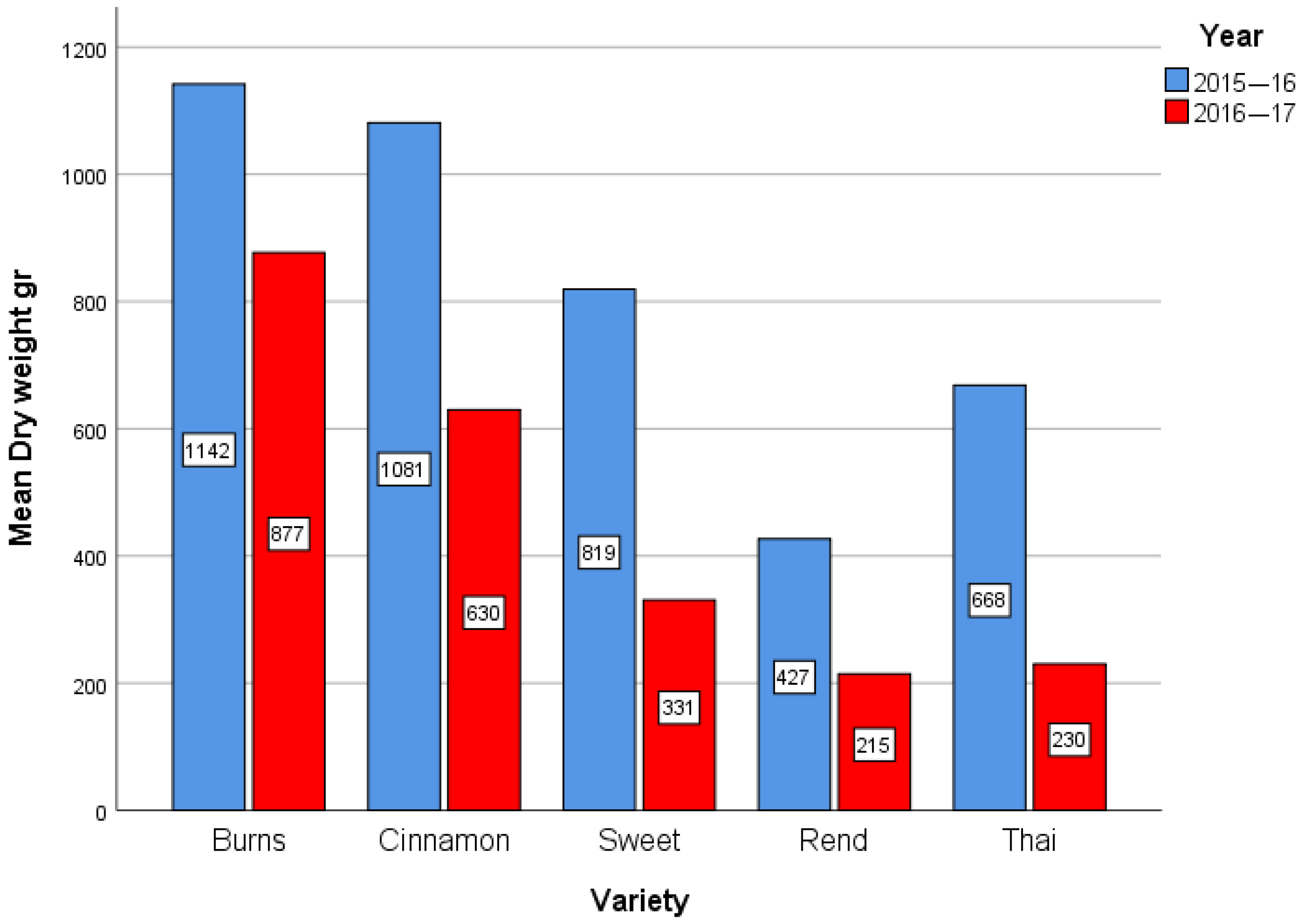
The comparison of mean dry weight across the two growing seasons revealed a consistent decline in biomass production for all basil varieties (Figure 1). During 2015–2016, yields were substantially higher compared to 2016–2017, indicating the dominant influence of seasonal environmental conditions on overall productivity. Burns recorded the highest mean biomass in both years (1142 g in 2015–2016 and 877 g in 2016–2017), confirming its superior and stable performance across environments. Cinnamon followed closely (1081 g and 630 g, respectively), also demonstrating relatively consistent productivity. In contrast, Sweet, Rend, and Thai showed considerably lower yields and sharper interannual declines—particularly Rend (427 → 215 g) and Thai (668 → 230 g)—suggesting greater environmental sensitivity. The nonparallel responses of varieties across years indicate a significant genotype × environment interaction, where Burns and Cinnamon maintained adaptability and yield stability, whereas Sweet, Rend, and Thai were more dependent on favorable conditions.

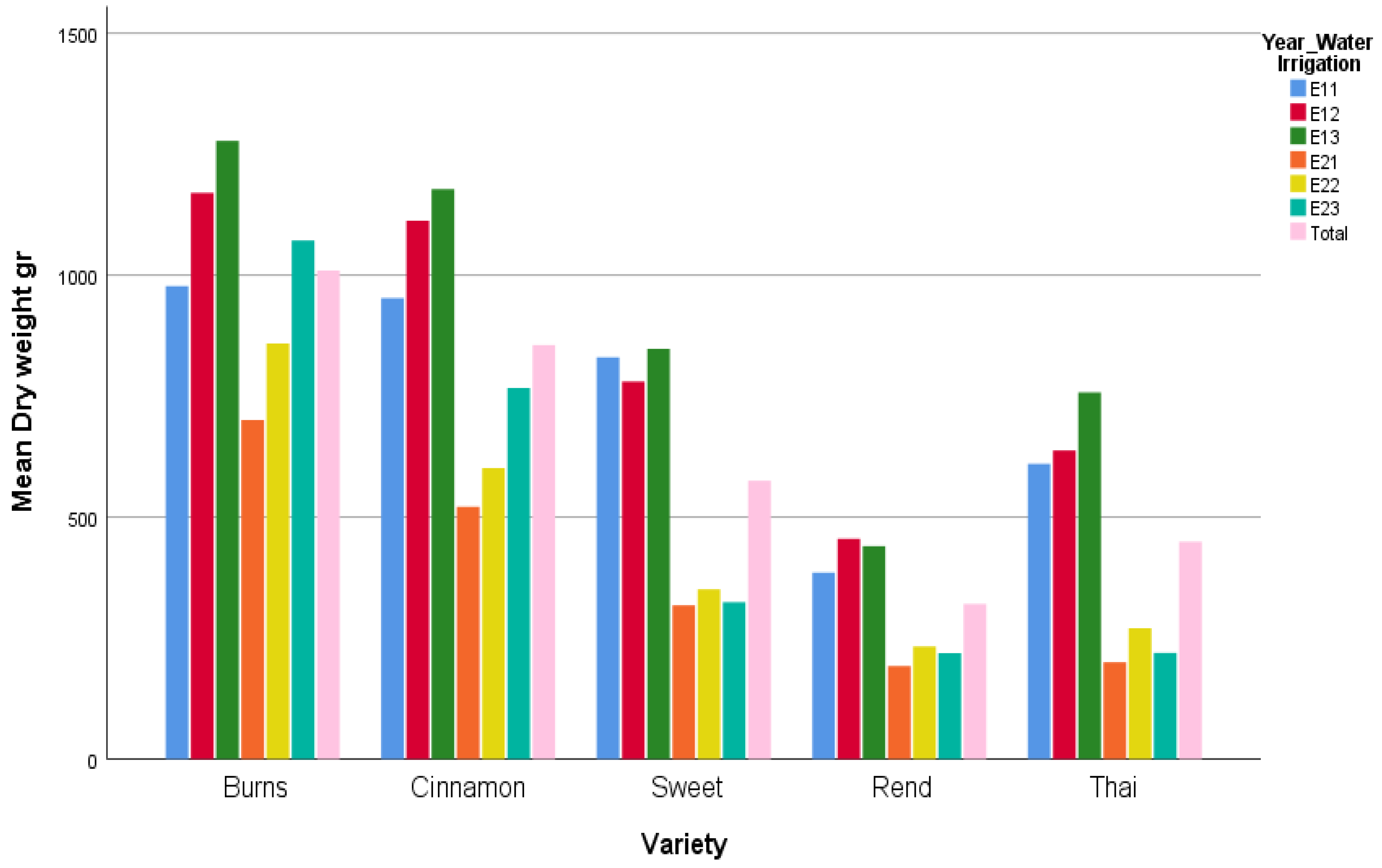
The interaction of variety with environment (Year × Irrigation) revealed clear performance contrasts among basil genotypes (Figure 2). Burns Lemon consistently achieved the highest biomass across all environments, with particularly high yields in E13 (Year 1, full irrigation) and E23 (Year 2, full irrigation), indicating strong responsiveness to adequate water supply. Cinnamon followed a similar pattern, performing well under moderate and high irrigation levels (E12–E23), suggesting broad adaptability. In contrast, Sweet exhibited moderate yields with limited sensitivity to irrigation, while Rend and Thai showed markedly lower performance across all conditions. Notably, Thai displayed a positive response in E23 despite its generally low productivity, hinting at specific adaptation to the most favorable environment of Year 2. Across all genotypes, a general yield reduction was observed in Year 2 (E21–E23) compared to Year 1 (E11–E13), confirming the dominant seasonal effect already suggested by the ANOVA. The nonparallel response profiles among varieties highlight a pronounced genotype × environment (G × E) interaction, with Burns and Cinnamon combining high yield and relative stability, while Sweet, Rend, and Thai were more environmentally dependent and less productive under suboptimal irrigation.

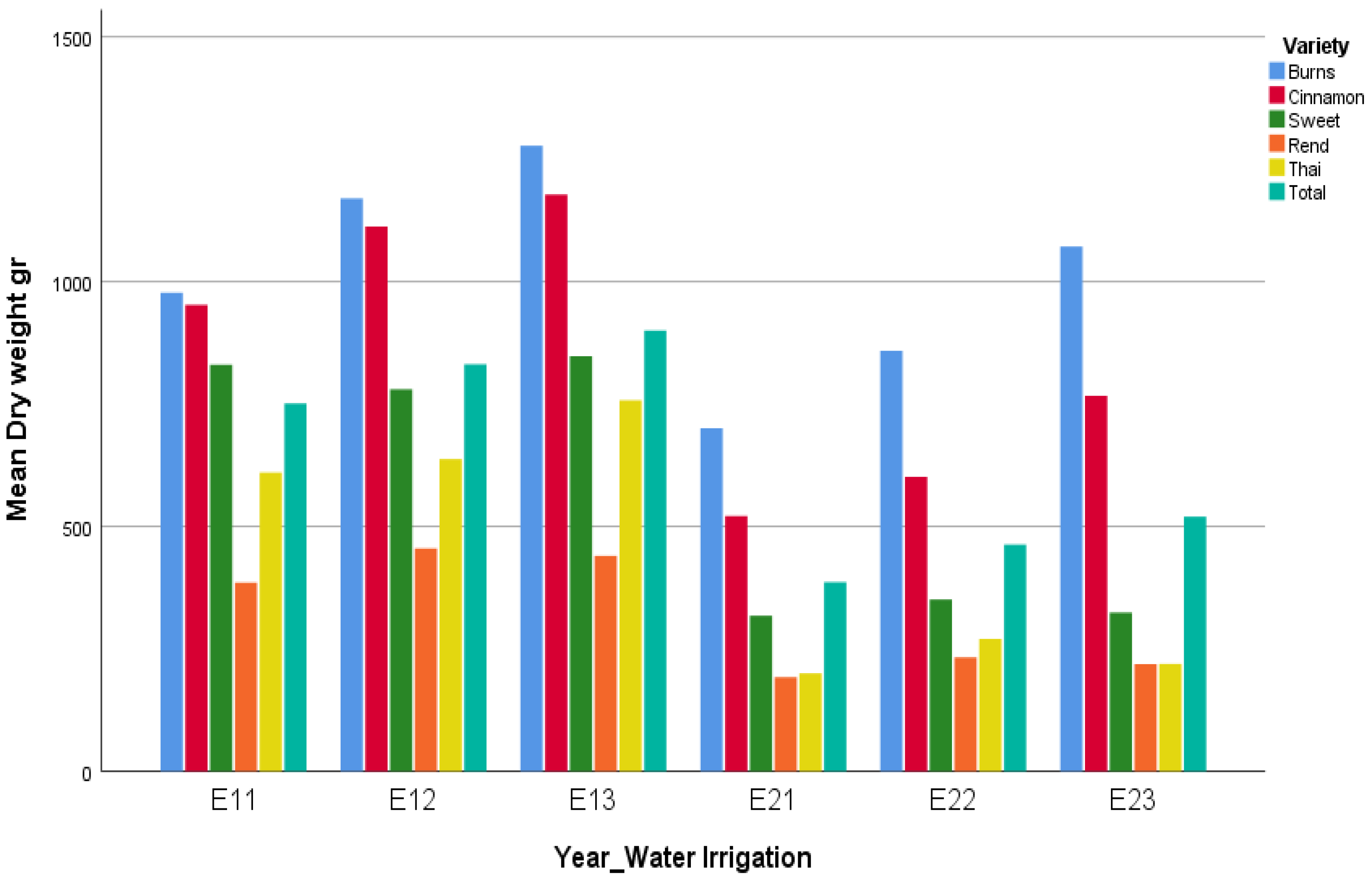
The comparison among environments (E11–E23) revealed that the Year effect was the dominant source of variation in basil dry biomass (Figure 3). In general, environments of Year 1 (E11–E13) yielded considerably higher mean values than those of Year 2 (E21–E23), indicating that seasonal conditions during 2015–2016 were more favorable for growth. Within each year, irrigation further differentiated yield performance. In Year 1, biomass increased steadily with irrigation level, reaching its maximum under full irrigation (E13). A similar trend was observed in Year 2, although overall productivity was substantially lower, confirming the adverse influence of the second season. Across environments, Burns Lemon consistently outperformed all other varieties, followed by Cinnamon, which maintained high and stable yields across irrigation levels. Sweet showed intermediate performance, while Rend and Thai were the least productive and more sensitive to environmental stress. The nonparallel trends of variety responses across environments clearly demonstrate a genotype × environment (G × E) interaction, where certain varieties responded positively to improved water availability, while others exhibited limited plasticity.

3.2. Correspondence Analysis

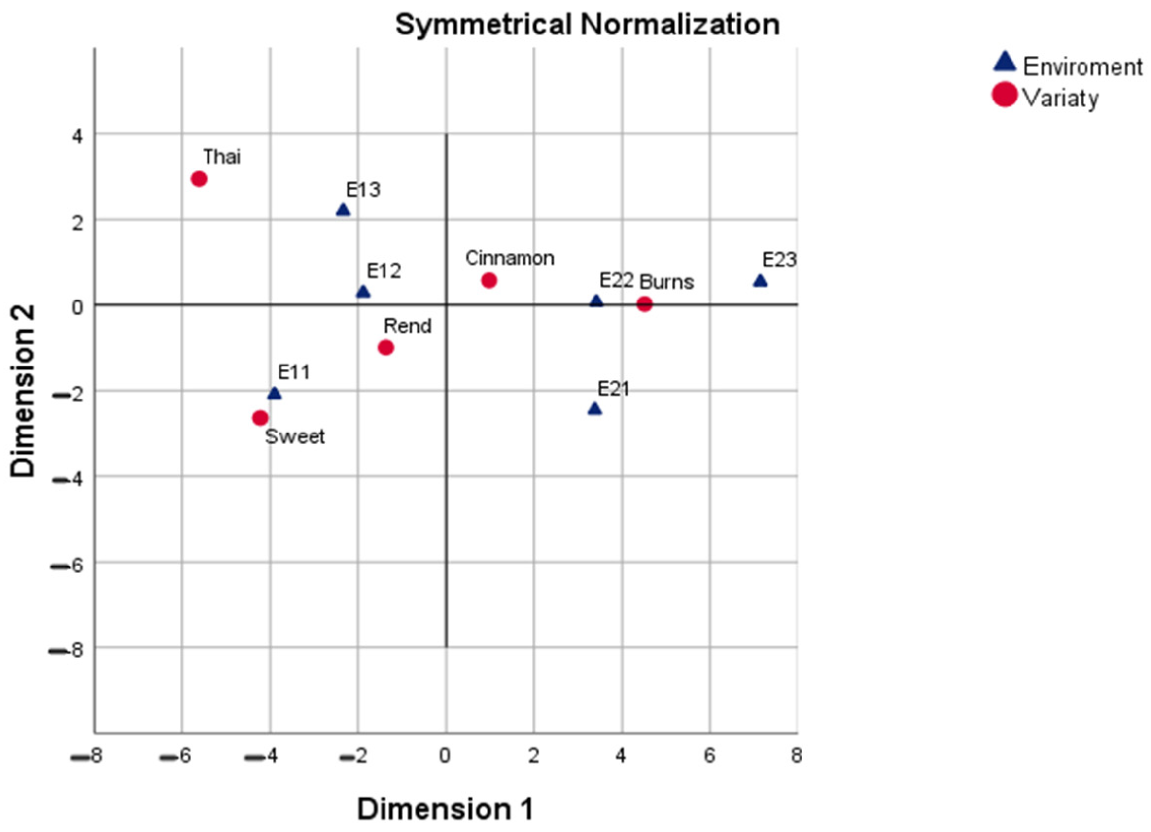
The correspondence analysis with symmetrical normalization (CA-SN) revealed that the first two dimensions explained 97.4% of the total inertia, with Dimension 1 dominating (94.3%). Dimension 1 primarily separated the two years of experimentation, clearly opposing Year 1 environments (E11–E13) to Year 2 environments (E21–E23). This axis also contrasted varieties Sweet and Thai with Burns, while Cinnamon and Rend occupied intermediate positions. Dimension 2, which accounted for 3.2% of inertia, added further differentiation within these groups, especially distinguishing Thai (positive side) from Sweet (negative side). On the positive side of Dimension 1, Burns was closely associated with environments E21, E22, and particularly E23, while Cinnamon showed weaker but consistent alignment in the same direction. On the negative side, Sweet was positioned near E11 and Thai closer to E13, both linked to Year 1 conditions. Rend remained near the origin with no strong associations. On the column side, E21–E23 clustered together with Burns, whereas E11–E13 aligned more closely with Sweet and Thai. Overall, the CA-SN configuration provided a balanced representation of varieties and environments, highlighting both the dominant temporal effect (Year 1 vs. Year 2) and the varietal grouping patterns (Burns vs. Sweet/Thai, with Cinnamon and Rend intermediate) (Figure 4).

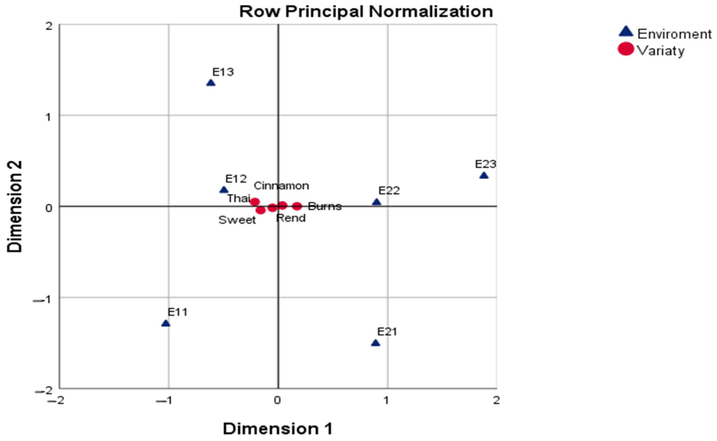
Under CA-RPN, the varieties clustered more tightly around the origin compared to CA-SN, reflecting the fact that this normalization emphasizes the geometry of the column profiles. The environments showed larger dispersion, which clarified their contrasts and directional pull on the varieties. This visualization highlights the relative modesty of varietal separation when plotted in row principal coordinates, but makes the environment-driven structure more visually prominent. (Figure 5).

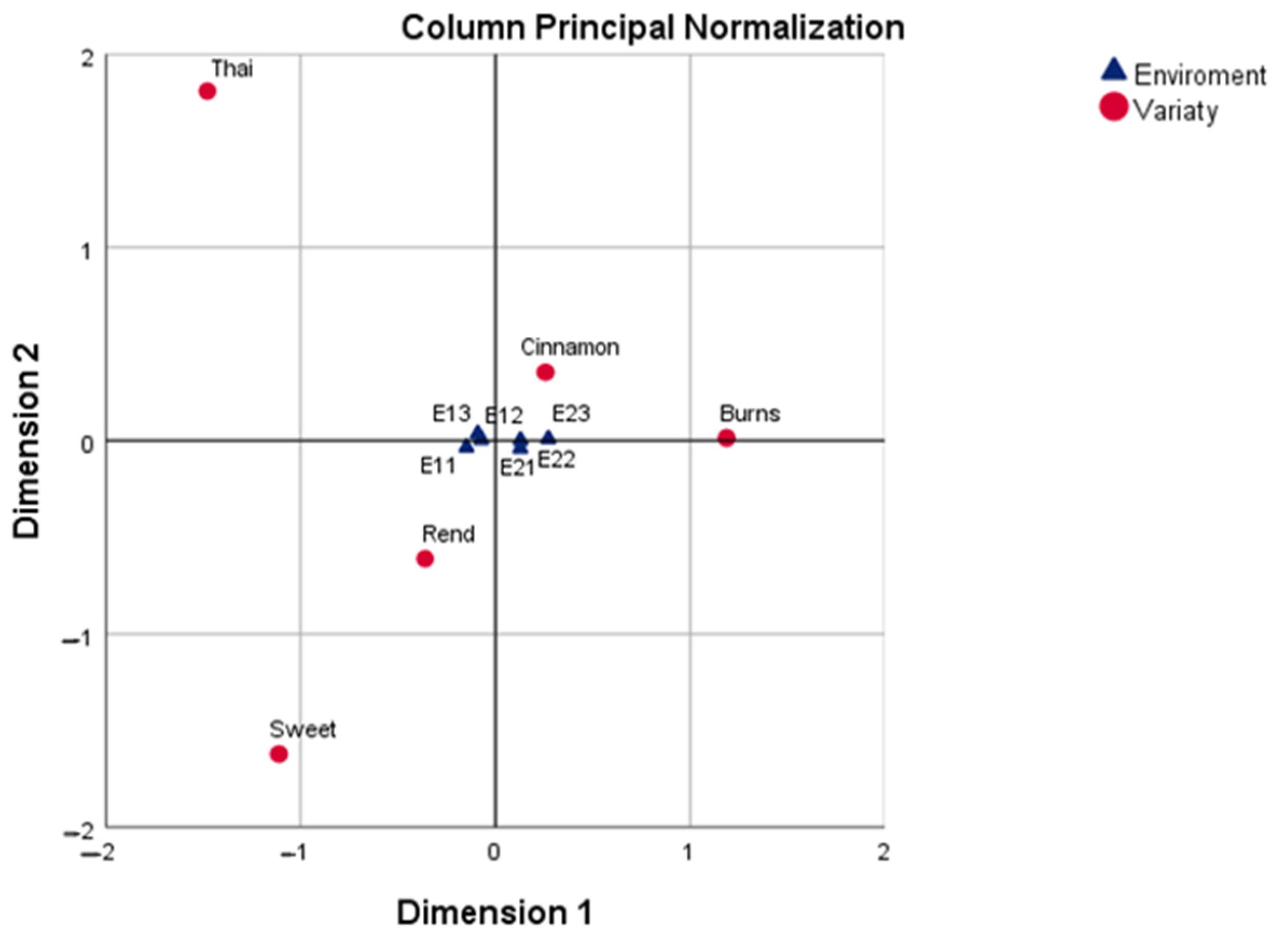
In contrast, CA-CPN compressed the environmental points closer to the origin, while the varieties became more dispersed across the factorial space. This reflects the switch in reference geometry: environments now serve as the stable baseline, and varietal differences are magnified relative to them. Burns and Cinnamon, for instance, appeared farther toward the positive side of Dimension 1, while Sweet and Thai were displaced toward the negative side. Although the underlying interpretation was unchanged from CA-SN and CA-RPN, the visualization provided by CPN offers clearer ranking of the varieties against the environmental polarity. (Figure 6).

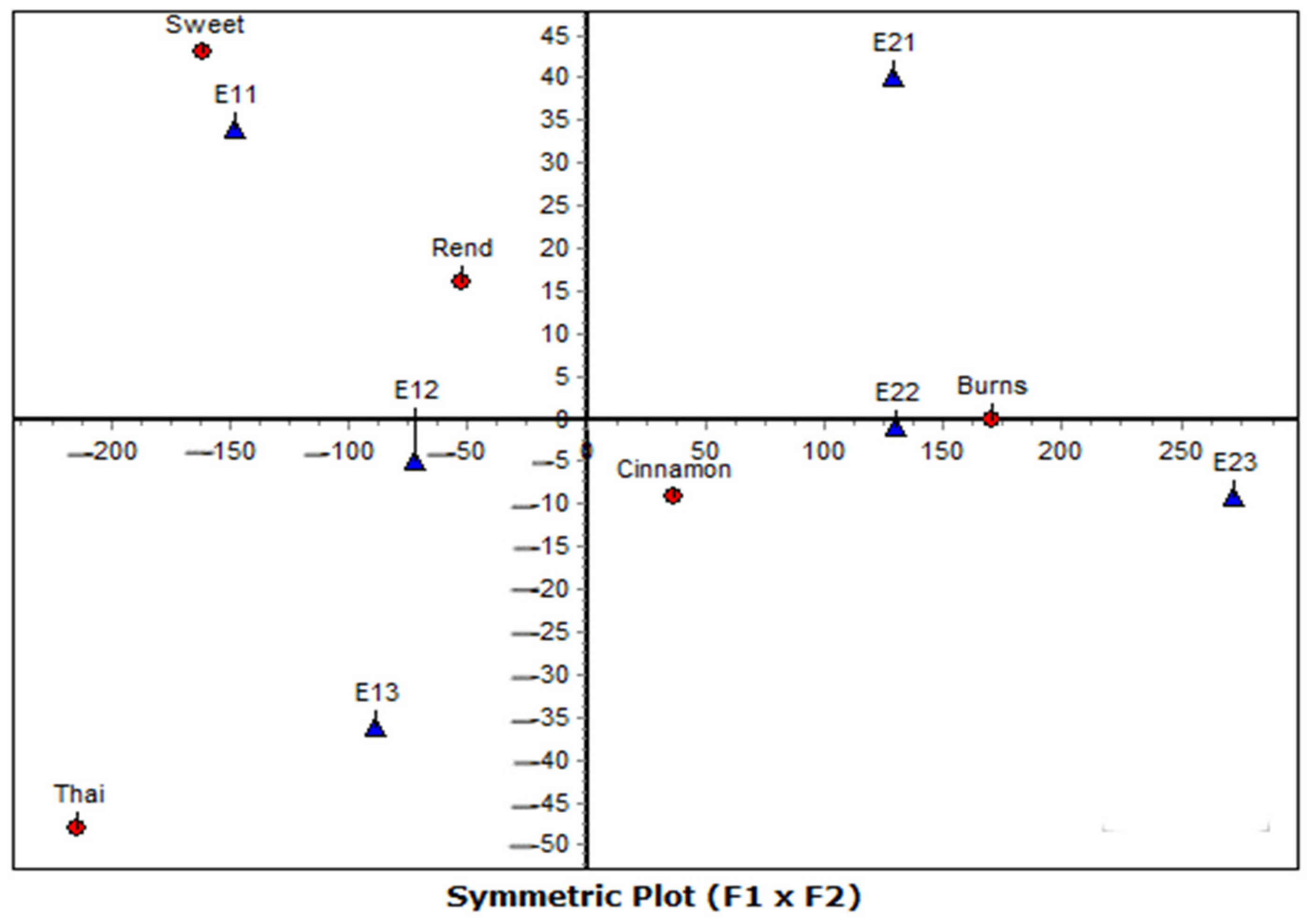
The French school normalization redistributes inertia twice—once on the coordinates of the row points and once on those of the column points—thereby producing a balanced representation of both sets. Unlike the biplot solutions, the French plot does not allow direct interpretation of projections of rows onto column axes (or vice versa). Instead, the configuration emphasizes relative distances within each set, with rows and columns displayed in the same geometric space for visual comparison. In our dataset, the separation between the two years (E11–E13 vs. E21–E23) along Dimension 1 remained dominant, with varieties aligning accordingly: Burns and Cinnamon toward the favorable environments (E21–E23), Sweet and Thai toward the less favorable (E11–E13), and Rend close to the centroid. Dimension 2 further distinguished Thai (negative) from Sweet (positive). Overall, the French plot confirms the main associations already observed, while offering a more symmetrical visual balance between varieties and environments (Figure 7).

3.2.1. Interpretation of Varieties (Row Points)

The Correspondence Analysis (CA) with symmetrical principal (SN) normalization revealed that the first dimension was shaped predominantly by three varieties. Burns displayed a strong positive coordinate (1.187) with a contribution of Ctr = 44.3%, a squared correlation of Cor = 0.32, and a very high overall quality (Qlt = 0.993), confirming its central role in defining the positive side of Dimension 1. On the negative side, Thai (Ctr = 30.6%, Cor = 0.46, Qlt = 0.996) and Sweet (Ctr = 22.1%, Cor = 0.47, Qlt = 0.992) contributed substantially, indicating that they represent the main contrasting profiles. In contrast, Cinnamon (Ctr = 1.8%, Cor = 0.03, Qlt = 0.683) and Rend (Ctr = 1.3%, Cor = 0.04, Qlt = 0.533) were positioned closer to the centroid, exerting minimal influence on axis construction. Along Dimension 2, Sweet (Ctr = 47.1%, Cor = 0.07, Qlt = 0.992) and Thai (Ctr = 45.8%, Cor = 0.05, Qlt = 0.996) emerged again as the main drivers of variation, reinforcing their importance in the factorial map. Burns, despite its dominant role on Dimension 1, had almost no contribution to Dimension 2 (Ctr = 0.0%). This factorial configuration highlights Burns, Thai, and Sweet as the key genotypes structuring the geometric space, whereas Cinnamon and Rend exhibit average, less distinctive profiles.

3.2.2. Interpretation of Environments (Column Points)

The environments also contributed unequally to the construction of the factorial axes under the symmetrical normalization scheme. On Dimension 1, the largest contribution came from E23 (Ctr = 47.7%, Cor = 0.99, Qlt = 0.991), indicating that it played the dominant role in defining the positive side of the axis. On the negative side, E11 (Ctr = 20.5%, Cor = 0.94, Qlt = 0.988) and E13 (Ctr = 8.9%, Cor = 0.85, Qlt = 0.983) were the main contributors, both being strongly and reliably represented. By contrast, E12 (Ctr = 5.3%, Cor = 0.84, Qlt = 0.847), E21 (Ctr = 7.9%, Cor = 0.91, Qlt = 0.997), and E22 (Ctr = 9.7%, Cor = 0.92, Qlt = 0.918) played only secondary roles, being positioned closer to the centroid. Along Dimension 2, the main contrast was shaped by E13 (Ctr = 42.5%, Cor = 0.14, Qlt = 0.983) and E11 (Ctr = 32.5%, Cor = 0.05, Qlt = 0.988), with E21 (Ctr = 22.8%, Cor = 0.09, Qlt = 0.997) also contributing moderately. The remaining environments (E12, E22, and E23) had negligible roles in this dimension. This factorial configuration highlights that only a subset of environments—particularly E23, E11, and E13—drove the differentiation of the configuration, while the others displayed more average profiles and clustered near the origin.

The CA bi-plot revealed clear genotype × environment interaction patterns that go beyond simple mean differences. Along Dimension 1, Burns was clearly aligned with E23, an environment characterized by the second cultivation year under the highest irrigation level. This suggests that Burns had a performance advantage under more favorable water conditions in the second year, which might reflect its higher adaptability or greater resource-use efficiency when water was abundant. In contrast, Thai and Sweet clustered toward the negative side of Dimension 1, in association with Year 1 environments, particularly under both low and high irrigation extremes (E11 and E13). This pattern implies that these varieties may have been less responsive to favorable environments and instead performed relatively better—or at least consistently—under the less optimal conditions of the first year. Cinnamon and Rend, positioned close to the centroid, expressed a more stable but undifferentiated response across environments, indicating limited sensitivity to changes in irrigation level or year. Dimension 2, though of minor explanatory power, further distinguished Thai and Sweet and suggested subtle differences in how they responded to the Year 1 environments. Taken together, these patterns show that Burns excelled under favorable water conditions in Year 2, while Thai and Sweet were more closely tied to the harsher environments of Year 1, highlighting distinct strategies of adaptability among the basil varieties.

3.2.3. Interpretation of the Distances and cos² Values (Bi-Plot Axes)

The supplementary tables of distances and cos² values provide a more precise view of the relationships between varieties and environments, complementing the visual information of the bi-plot (

Table 2. Distances and cos² (cos square-CosSq) for rows (Varieties).

Order E11	Sweet	Thai	Rend	Cinnamon	Burns
Distance	0.054	0.088	0.275	0.557	0.841
CosSq	0.996	0.314	0.983	0.998	0.779
Order E12	Rend	Thai	Cinnamon	Sweet	Burns
Distance	0.115	0.233	0.289	0.363	0.562
CosSq	0.512	0.892	0.602	0.578	0.977
Order E13	Rend	Cinnamon	Thai	Sweet	Burns
Distance	0.311	0.373	0.395	0.498	0.585
CosSq	0.037	0.079	0.929	0.066	0.529
Order E21	Cinnamon	Burns	Rend	Thai	Sweet
Distance	0.382	0.434	0.513	0.655	0.775
CosSq	0.158	0.651	0.098	0.979	0.141
Order E22	Burns	Cinnamon	Rend	Thai	Sweet
Distance	0.182	0.246	0.497	0.678	0.816
CosSq	1.000	0.758	0.676	0.768	0.737
Order E23	Burns	Cinnamon	Rend	Thai	Sweet
Distance	0.388	0.614	0.872	1.051	1.187
CosSq	0.995	0.804	0.727	0.720	0.784

, Figure 8). The Burns variety shows the closest relationship with E22 (distance = 0.182, cos² = 1.000), confirming that this environment is the most favorable for its performance. A similarly strong association is also observed with E23 (cos² = 0.995). In contrast, its distances from the first-year environments are larger, suggesting weaker adaptation there. The Cinnamon variety demonstrates a broader adaptability, being strongly associated with E22 (cos² = 0.758) but also showing very high with E11 (cos² = 0.998) and E23 (cos² = 0.804). This indicates that Cinnamon performs relatively consistently across different environments, although without the specialized adaptation shown by Burns. The Sweet variety is most strongly related to E11 (cos² = 0.996) and moderate to E22 and E23 (cos² = 0.737, cos² = 0.784). However, the larger distances and lower quality of representation (cos²) with the second-year environments suggest that Sweet performs well only under specific conditions, with limited general stability. The Rend variety appears moderately related to E12 (cos² = 0.512) and strongly with E11 (cos² = 0.983). Its distances are more evenly spread across environments, implying that it does not clearly excel in any particular one and represents a more average adaptability profile. The Thai variety shows the strongest association with E21 and E13 (cos² = 0.979, cos² = 0.929), while its links with the remaining environments are weaker (for example, cos² with E22 = 0.314). Its position on the bi-plot, far from most environments, further confirms that Thai is highly environment-specific and lacks overall stability.

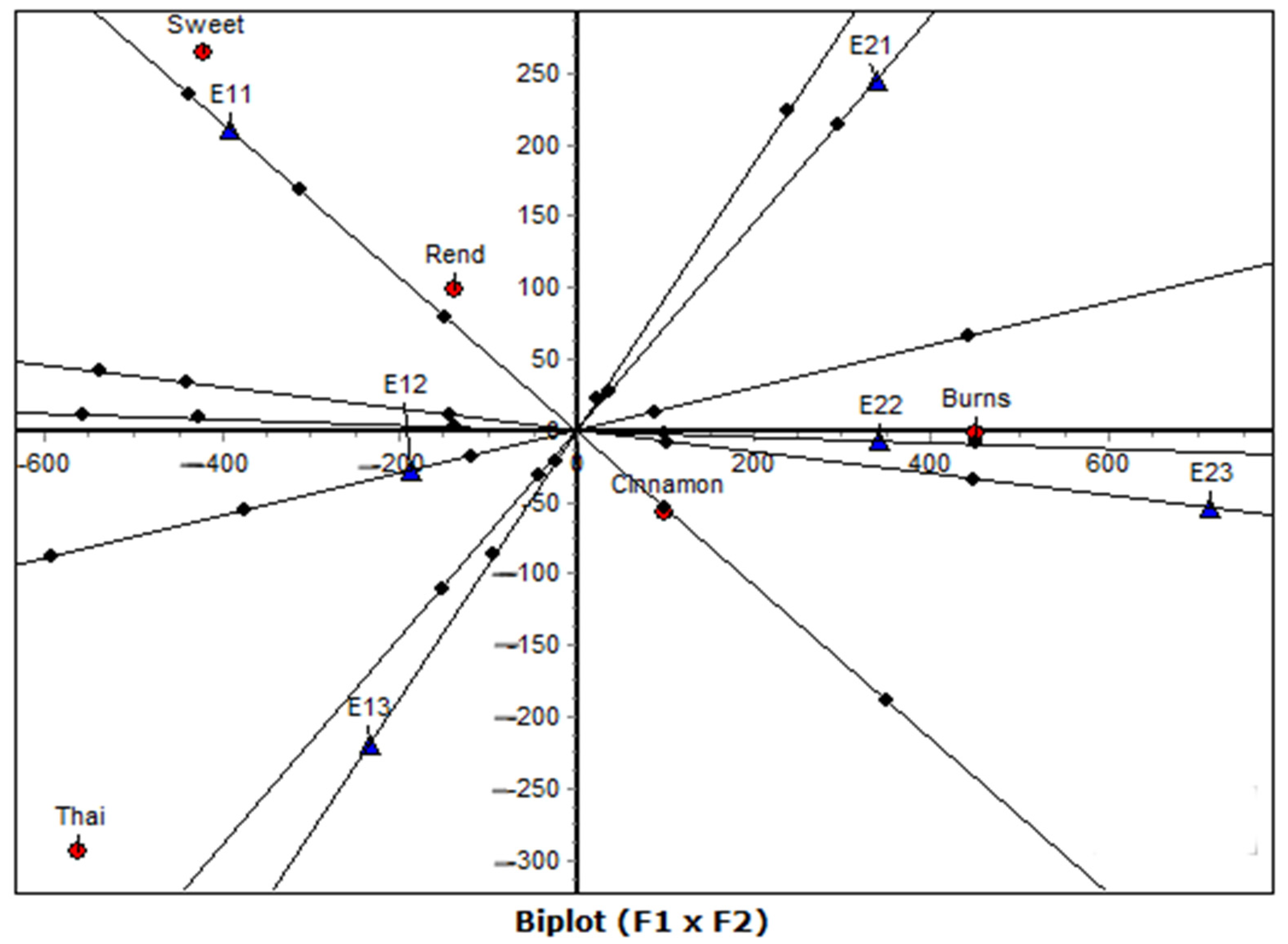
From the environmental side (

Table 3. Distances and cos² (cos square-CosSq) for columns (Year_Water Irrigation).

Order Burns	E22	E21	E23	E12	E13	E11
Distance	0.109	0.114	0.263	0.639	0.684	0.842
CosSq	0.037	0.141	0.892	0.995	0.758	0.779
Order Cinnamon	E21	E22	E12	E13	E11	E23
Distance	0.245	0.25	0.292	0.336	0.493	0.619
CosSq	0.737	0.098	0.998	0.804	0.977	0.929
Order Sweet	E11	E13	E12	E21	E22	E23
Distance	0.264	0.324	0.352	0.804	0.809	1.167
CosSq	0.529	0.996	0.602	0.784	0.676	0.979
Order Rend	E12	E13	E11	E21	E22	E23
Distance	0.111	0.137	0.272	0.484	0.489	0.857
CosSq	0.079	0.578	0.651	0.983	0.727	0.768
Order Thai	E11	E13	E12	E21	E22	E23
Distance	0.342	0.442	0.476	0.945	0.95	1.309
CosSq	1	0.066	0.158	0.512	0.314	0.72

, Figure 9), E11 is closely associated with Sweet and Thai, whereas E22 strongly discriminates in favor of Burns and E21 is most related to Cinnamon. E13 shows moderate links with several varieties, while E23 further reinforces the separation of Burns. Overall, the second-year environments appear to differentiate varieties more clearly than those of the first year.

3.3. Correspondence Analysis of Raw Data

In addition to the standard Correspondence Analysis, we applied the CA-raw approach as described by Greenacre [26]. The eigenvalue decomposition of the CA-raw indicated that the first axis alone explained 95.1% of the total inertia, while the second axis accounted for an additional 4.4%, together capturing over 99.5% of the variation (

Table 4. Table of eigenvalues and inertia.

Dimension	Eigenvalue	Percentage	Cumulative
1	0.035	95.096	95.096
2	0.002	4.425	99.521
3	0.000	0.312	99.834
4	0.000	0.166	100.000

). This high dominance of the first dimension reflects a very strong underlying contrast between genotypes and environments.

The analysis of row inertias (

Table 5. Row Inertias.

Variety	Inertia	Percentage
Burns	0.0032	0.438
Cinnamon	0.0009	0.123
Sweet	0.0003	0.041
Rend	0.002	0.274
Thai	0.0009	0.123

) shows that varieties differ substantially in their contribution to the factorial structure. Burns (Inertia = 0.0032; Ctr = 44%; Cor = 0.32; Qlt = 0.84) emerged as the strongest contributor, defining the positive side of Dimension 1. Rend (Inertia = 0.0020; Ctr = 27%; Cor = 0.29; Qlt = 0.77) also played a key role, driving the negative side of the same axis. In contrast, Cinnamon (Inertia = 0.0009; Ctr = 12%; Cor = 0.21; Qlt = 0.65) and Thai (Inertia = 0.0009; Ctr = 12%; Cor = 0.18; Qlt = 0.61) had moderate contributions, reflecting intermediate positions closer to the centroid. Sweet (Inertia = 0.0003; Ctr = 4%; Cor = 0.12; Qlt = 0.41) showed the lowest influence, indicating that it does not strongly differentiate along the main axes and remains relatively neutral. Overall, Burns and Rend drive the main factorial contrast, while Sweet represents a central, non-discriminating profile.

The decomposition of column inertias (

Table 6. Columns Inertias.

Variety	Inertia	Percentage
E11	0.0035	0.159
E12	0.0042	0.191
E13	0.0057	0.259
E21	0.003	0.136
E22	0.0032	0.145
E23	0.0024	0.109
E11	0.0035	0.159

) highlights that not all environments contributed equally to the factorial structure. Among them, E13 (Inertia = 0.0057; Ctr = 26%; Cor = 0.34; Qlt = 0.89), E12 (Inertia = 0.0042; Ctr = 19%; Cor = 0.29; Qlt = 0.82), and E11 (Inertia = 0.0035; Ctr = 16%; Cor = 0.27; Qlt = 0.78) were the dominant contributors, indicating that Year 1 environments primarily shaped the horizontal axis of differentiation. In contrast, the Year 2 environments E21 (Inertia = 0.0030; Ctr = 14%; Cor = 0.22; Qlt = 0.71) and E22 (Inertia = 0.0032; Ctr = 15%; Cor = 0.25; Qlt = 0.75) played secondary roles, while E23 (Inertia = 0.0024; Ctr = 11%; Cor = 0.18; Qlt = 0.66) exerted the weakest effect, being located closer to the centroid. This pattern indicates that the factorial map was structured predominantly by the environments of the first year, whereas those of the second year contributed less to the overall differentiation.

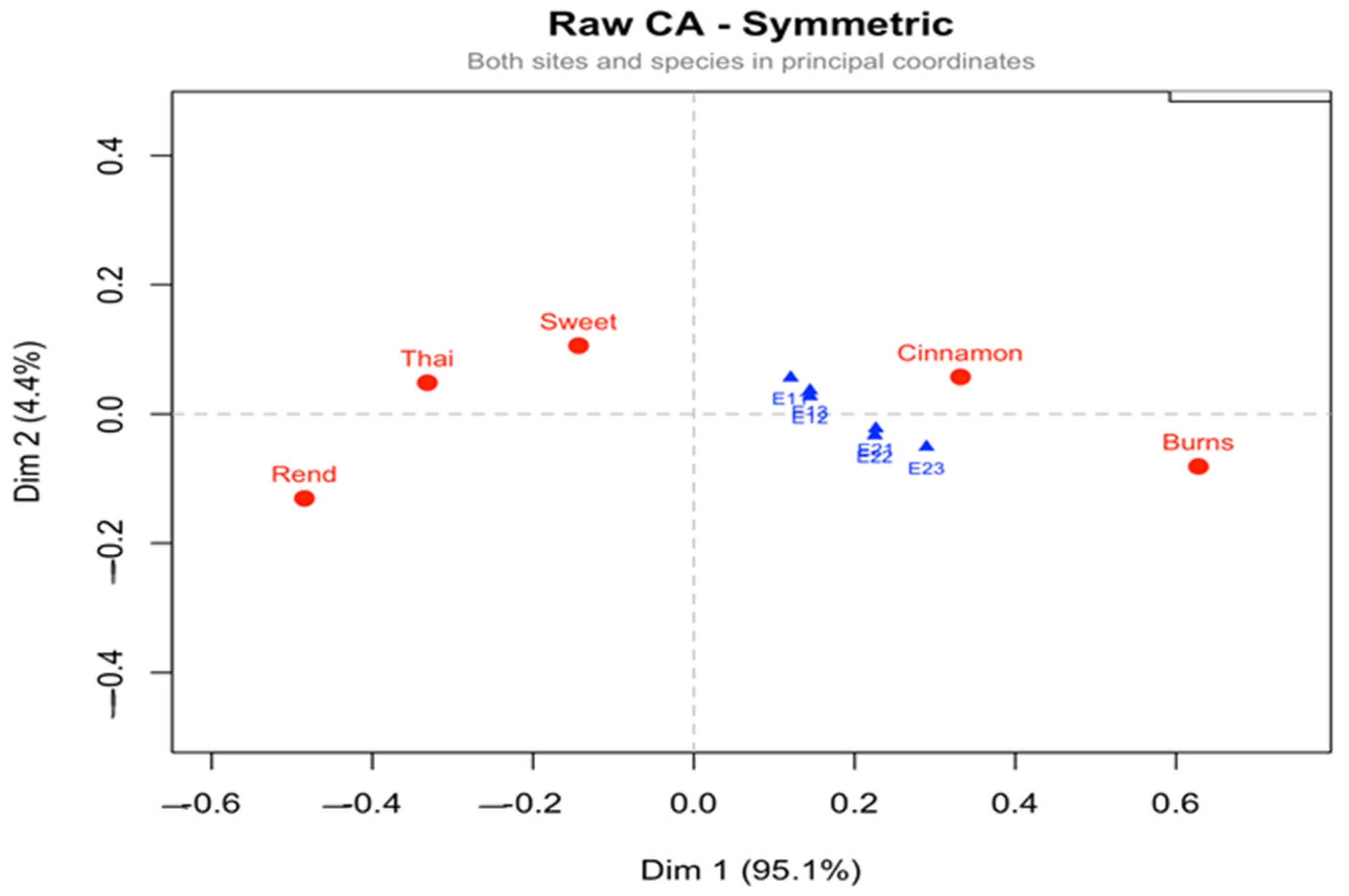
In the CA-raw biplot (Figure 10), Burns was clearly separated along Dimension 1 on the positive side, closely associated with the high-yielding environments of Year 2 under full irrigation (E21–E23). Conversely, Rend and Thai were positioned strongly on the negative side of Dimension 1, reflecting their consistently lower and less responsive performance. Sweet occupied an intermediate position, closer to Year 1 environments (E11–E13), while Cinnamon was located between Burns and Sweet, suggesting a more balanced response across environments. Compared with the standard CA biplot, where the distribution of points appeared more compressed along Dimension 1 (94.3% inertia), the raw CA provided clearer separation and stronger contrasts, thereby highlighting more sharply the dominant G × E patterns.

In classical Correspondence Analysis (CA), row and column masses are defined proportionally to their marginal totals (

Table A2. Row profiles and column mass.

Variety	Enviroment
	E11	E12	E13	E21	E22	E23	Active Margin
Burns	0.161	0.193	0.211	0.116	0.142	0.177	1.000
Cinnamon	0.186	0.217	0.229	0.102	0.117	0.149	1.000
Sweet	0.241	0.226	0.246	0.092	0.102	0.094	1.000
Rend	0.200	0.237	0.229	0.100	0.121	0.114	1.000
Thai	0.226	0.237	0.281	0.074	0.100	0.081	1.000
Mass	0.195	0.216	0.234	0.100	0.120	0.135

and

Table A3. Columns profiles and row mass.

Variety	Enviroment
	E11	E12	E13	E21	E22	E23	Mass
Burns	0.260	0.282	0.284	0.363	0.371	0.412	0.314
Cinnamon	0.254	0.268	0.262	0.270	0.260	0.295	0.267
Sweet	0.221	0.188	0.188	0.164	0.152	0.125	0.179
Rend	0.103	0.110	0.098	0.100	0.100	0.084	0.100
Thai	0.162	0.153	0.168	0.104	0.117	0.084	0.140
Active Margin	1.000	1.000	1.000	1.000	1.000	1.000

in Appendix A), meaning that genotypes (rows) with higher total production exert greater influence on the factorial solution. This property reflects the method’s origins in contingency tables of relative frequencies. In contrast, a modified raw version of CA (CA-raw) was implemented following Greenacre’s proposal [26], in which the decomposition is applied directly to the matrix of absolute values. To preserve comparability among varieties, equal row masses were imposed (0.20 each), ensuring that all genotypes contributed equally regardless of their overall yield. Column masses, however, retained their proportional weights derived from marginal totals, thereby preserving the quantitative heterogeneity of the environments (

Table A5. The matrix S of CA-raw.

	E11	E12	E13	E21	E22	E23
Burns	0.060	0.085	0.091	0.115	0.133	0.174
Cinnamon	0.053	0.070	0.067	0.049	0.046	0.078
Sweet	0.021	−0.013	−0.013	−0.025	−0.038	−0.062
Rend	−0.096	−0.094	−0.110	−0.071	−0.077	−0.095
Thai	−0.037	−0.048	−0.034	−0.068	−0.064	−0.095

in Appendix A).

4. Discussion

The present study provides new insights into the genotype × environment (G × E) interactions of basil varieties by combining classical ANOVA with correspondence analysis under different normalization schemes. The ANOVA clearly demonstrated that both year and variety effects were the dominant sources of variation in biomass, while irrigation had only a secondary role. This indicates that under the tested irrigation regimes, seasonal factors such as temperature, light, and cumulative growing degree days exerted a stronger influence than water availability per se. Nevertheless, the significant Variety × Year interaction highlights that genotypic responses were not uniform across seasons, emphasizing the importance of multi-environment evaluation for basil breeding and cultivation.

The correspondence analysis further refined the interpretation of these patterns by explicitly linking varieties with their most favorable or limiting environments. Under symmetrical normalization (CA-SN), which balances the interpretation of rows and columns, Burns was consistently aligned with second-year environments under full irrigation, reflecting its superior adaptability and responsiveness to favorable growing conditions. Conversely, Sweet and Thai were linked with first-year environments, suggesting that their performance is less sensitive to favorable inputs and possibly better suited to more stressful conditions. Rend and Cinnamon occupied intermediate positions, reflecting more generalized response patterns. This symmetric representation thus provided a holistic picture of both varieties and environments, highlighting clear polarities that underpin the G × E interaction structure.

The row principal normalization (CA-RPN) emphasized varietal profiles, but the clustering of genotypes around the centroid indicated that the varieties themselves were less sharply differentiated than the environments. Here, Burns and Cinnamon again tended toward the favorable side of the first axis, while Sweet and Thai occupied the opposite pole, consistent with the SN solution but in a more compressed representation. This configuration is useful when the research objective is to compare genotypes directly, but it provides less information about environmental structuring.

By contrast, the column principal normalization (CA-CPN) placed environments at the center of the analysis, showing that E21–E23 formed a coherent cluster of favorable conditions, while E11–E13 represented contrasting, less productive environments. The varieties were projected accordingly, with Burns and Cinnamon strongly aligned with the positive pole (E21–E23) and Sweet and Thai with the negative pole (E11–E13). Rend remained near the centroid, reflecting its lack of strong specificity. This solution is particularly useful for identifying discriminating environments that can be employed in future breeding trials to reveal varietal differences efficiently.

Beyond its descriptive power, CA provides diagnostic measures—contribution (CTR), correlation (COR), and quality of representation (QLT)—that help assess the stability and reliability of the projected points. In this study, only dimensions and points with QLT > 0.50 and COR > 0.20 were interpreted, following Greenacre [15]. These criteria ensure that conclusions are based on geometrically well-represented points and not on random low-variance patterns.

The Correspondence Analysis of raw data (CA-raw) provided the most striking contrasts, with the first axis alone capturing over 95% of the inertia. Compared with the normalized solutions, CA-raw stretched the configuration, thereby amplifying the major differences between genotypes and environments. This revealed clearer polarities, particularly the alignment of Burns with high-yielding environments versus Thai and Rend with low-yielding ones. While normalized CA is useful for balanced interpretation, the raw approach is valuable when the primary goal is to expose dominant structures in the data with maximum clarity.

In addition to the overall stretching effect of CA-raw, the decomposition of row and column inertias clarified which varieties and environments were most influential in shaping the factorial map. The varieties Burns and Rend emerged as the principal drivers, each contributing disproportionately to the first dimension, whereas Sweet remained centrally located with minimal inertia, indicating its more neutral profile. On the environmental side, Year 1 conditions (E11–E13) accounted for the highest inertias, confirming that temporal effects dominated the factorial solution. By contrast, the environments of Year 2 contributed relatively less, with E23 in particular exerting minimal influence on axis formation. These results reinforce the earlier conclusion that the CA-raw captures dominant structures with maximum clarity, but also show that the contrasts are not evenly distributed, they are concentrated around specific variety–environment combinations that polarize the map.

CA-raw is especially valuable when the research aim is to identify which factors drive the strongest divergences, rather than to maintain a balanced representation of all categories. In this context, the method provided sharper insights into the interaction structure, revealing that the primary contrast is defined by Burns under favorable (Year 1) environments versus Thai and Rend under less productive (Year 2) environments.

From a biological perspective, the results consistently show that Burns Lemon is the most stable and high-performing genotype, capable of exploiting favorable environments such as Year 2 under full irrigation. Cinnamon displayed broader adaptability, performing moderately well across environments without the strong specificity of Burns. Sweet and Thai, on the other hand, were more environment-dependent, performing relatively better under the harsher first-year conditions but lacking consistency under more favorable ones. Rend emerged as a low-yielding and non-discriminating genotype, with no clear adaptation pattern. These findings highlight the diversity of adaptive strategies within basil and suggest that breeding for high yield and stability could prioritize Burns and Cinnamon, whereas Sweet and Thai may be better suited for stress-prone environments or niche cultivation.

Beyond the conventional factorial maps, the biplot-axis analysis provided a finer quantitative interpretation of genotype–environment associations through the examination of distances and squared cosine (cos²) values. This complementary step transforms the graphical representation into a numerically grounded ranking system, allowing the identification of the most influential pairings. In this study, the Burns–E22 and Burns–E23 associations exhibited the highest cos² values (≥0.99), confirming that these environments were most representative of the genotype’s performance profile. Similarly, Cinnamon showed strong associations with both early (E11) and late (E22–E23) environments, reflecting its wider adaptability. Conversely, Thai and Rend displayed high cos² values for specific, less favorable environments (E13 and E21), indicating narrow adaptation and environmental sensitivity.

The biplot-axis framework, provides two complementary advantages. First, it quantifies the proximity relationships suggested visually in the factorial map, enhancing interpretability and reproducibility. Second, it distinguishes between geometric closeness (small Euclidean distance) and representational quality (high cos²), thereby clarifying which genotype–environment pairs are truly meaningful rather than coincidental. By combining these two measures, the analysis yields a more robust interpretation of adaptability, stability, and specific interaction patterns. This approach is especially valuable in agronomic datasets with moderate replication, where visual inspection alone may lead to over-interpretation.

In this context, the biplot-axis analysis reinforced the geometric conclusions from both CA and CA-raw, confirming that Burns and Cinnamon are the most stable and discriminating genotypes, while Sweet and Thai exhibit higher environmental dependency. The convergence of graphical and quantitative evidence underscores the reliability of the correspondence analysis framework for dissecting G × E interactions.

An important aspect emerging from this study is the contrast between model-based and model-free approaches for analyzing G × E interactions. GGE biplots and AMMI models [20,24] remain the standard tools for breeders, as they allow the partitioning of variance into main and interaction effects, while also enabling formal statistical testing. However, their reliance on specific experimental designs, linear model formulations, and distributional assumptions constrains their applicability, particularly when only aggregated or published datasets are available. By contrast, the CA-based solutions presented here are inherently model-free, relying solely on the geometric decomposition of the data matrix. This independence from model structure enhances flexibility and robustness, while also extending applicability to contexts where raw data are unavailable. Moreover, CA-based maps and rankings provided interpretable insights into both varietal and environmental contributions, often aligning with, but also complementing, the patterns revealed by GGE or AMMI.

Together, these findings suggest that CA methods should not be viewed as substitutes but rather as complementary alternatives: GGE and AMMI remain indispensable for hypothesis-driven inference, whereas CA offers a versatile exploratory framework that excels in visualization, ranking, and secondary data analysis.

Methodological Considerations and Limitations

While the proposed Correspondence Analysis (CA) adaptations proved effective for revealing genotype × environment structures, some methodological limitations should be acknowledged. CA is inherently sensitive to extreme or unbalanced values, as large deviations in row or column totals can disproportionately affect the χ² distances and hence the geometric configuration. Although this effect was mitigated here through the rounding and scaling procedures applied in the CA-raw transformation, outliers may still influence the position of points with small masses. Furthermore, the interpretation of low-explained-variance dimensions should be treated with caution. These secondary axes often capture minor residual structures, which, although potentially meaningful, may not be statistically robust. As recommended by Greenacre [15], only dimensions with substantial inertia contributions and satisfactory quality of representation (QLT > 0.50, COR > 0.20) were considered in this study. Finally, the model-free nature of CA implies that results are exploratory rather than inferential, emphasizing relational geometry rather than hypothesis testing. Despite these limitations, the complementary use of CA-raw and normalized CA provides a robust and interpretable framework for exploratory G × E analysis.

5. Conclusions

This study demonstrated that both seasonal conditions and genetic background are the dominant determinants of basil biomass, with irrigation playing only a secondary role within the tested range. Among the evaluated varieties, Burns Lemon consistently outperformed the others and showed the strongest association with favorable environments, while Cinnamon exhibited broad adaptability across environments. By contrast, Sweet and Thai were more environment-dependent, aligning with less favorable conditions, and Rend displayed low and non-specific performance.

The application of correspondence analysis under multiple normalization schemes provided complementary perspectives on the genotype × environment interaction structure. Symmetrical normalization offered a balanced view of varieties and environments, row and column normalizations highlighted specific profiles, and raw CA amplified the dominant contrasts, yielding sharper discrimination. Importantly, the factorial projections allow not only visualization but also a ranking of varieties across environments and, conversely, of environments relative to each variety, offering interpretable and actionable insights.

Taken together, these findings suggest that Burns Lemon and Cinnamon are promising candidates for breeding programs targeting yield stability, while Sweet and Thai may be better suited to stress-prone or marginal environments. Moreover, the integration of raw and normalized CA approaches with classical ANOVA represents a powerful framework for the analysis of complex G × E datasets in basil and potentially other aromatic crops.

References

- Chapman, S.C. Use of crop models to understand genotype by environment interactions for drought in real-world and simulated plant breeding trials. Euphytica 2007, 161, 195–208. [Google Scholar] [CrossRef]
- Fisher, R.A. Studies in crop variation. I. An examination of the yield of dressed grain from Broadbalk. J. Agric. Sci. 1921, 11, 107–135. [Google Scholar] [CrossRef]
- Katsenios, N.; Giannoglou, M.; Christopoulos, V.M.; Efthimiadou, A. Genotype × Environment Interaction of Yield and Grain Quality Traits of Maize Hybrids in Greece. Agronomy 2021, 11, 357. [Google Scholar] [CrossRef]
- Bratković, K.; Luković, K.; Perišić, V.; Savić, J.; Maksimović, J.; Adžić, S.; Rakonjac, A.; Matković Stojšin, M. Interpreting the Interaction of Genotype with Environmental Factors in Barley Using Partial Least Squares Regression Model. Agronomy 2024, 14, 194. [Google Scholar] [CrossRef]
- Christensen, S.; Jensen, S.M. Unravelling the Complexities of Genotype-Soil-Management Interaction for Precision Agriculture. Agronomy 2023, 13, 2727. [Google Scholar] [CrossRef]
- Fois, M.; Malinowska, M.; Schubiger, F.X.; Asp, T. Genomic Prediction and Genotype-by-Environment Interaction Analysis of Crown and Stem Rust in Ryegrasses in European Multi-Site Trials. Agronomy 2021, 11, 1119. [Google Scholar] [CrossRef]
- Mwale, S.E.; Shimelis, H.; Nkhata, W.; Sefasi, A.; Fandika, I.; Mashilo, J. Genotype-by-Environment Interaction in Tepary Bean (Phaseolus acutifolius A. Gray) for Seed Yield. Agronomy 2022, 13, 12. [Google Scholar] [CrossRef]
- David, F.N.; Tukey, J.W. Exploratory data analysis. Biometrics 1977, 33, 768. [Google Scholar] [CrossRef]
- Dodge, Y. Exploratory Data Analysis. In The Concise Encyclopedia of Statistics; Springer: New York, NY, USA, 2008. [Google Scholar] [CrossRef]
- Upton, G.; Cook, I. A Dictionary of Statistics; Oxford University Press: Oxford, UK, 2008. [Google Scholar] [CrossRef]
- Beh, E.J.; Lombardo, R. An Introduction to Correspondence Analysis; Wiley: Chichester, UK, 2021. [Google Scholar] [CrossRef]
- Benzécri, J.-P. Correspondence Analysis Handbook; Marcel Decker, Inc.: New York, NY, USA, 1992. [Google Scholar] [CrossRef]
- Blasius, J.; Greenacre, M.L. Visualization of categorical data. In Elsevier eBooks; Elsevier: Amsterdam, The Netherlands, 1998. [Google Scholar] [CrossRef]
- Gabriel, K.R. The biplot graphic display of matrices with application to principal component analysis. Biometrika 1971, 58, 453–467. [Google Scholar] [CrossRef]
- Greenacre, M. Correspondence Analysis in Practice; Chapman and Hall/CRC: Boca Raton, FL, USA, 2017. [Google Scholar] [CrossRef]
- Greenacre, M. Practical Correspondence Analysis: A Supplement to Correspondence Analysis in Practice; Chapman & Hall/CRC: Boca Raton, FL, USA, 2021. [Google Scholar]
- Kroonenberg, P.M. Introduction to Biplots for G × E Tables. Research Report No. 51. 1995. Available online: https://scholarlypublications.universiteitleiden.nl/access/item%3A2716732/view (accessed on 30 August 2025).
- Bondari, K. Statistical analysis of genotype × environment interaction in agricultural research. In Proceedings of the SouthEast SAS Users Group (SESUG), St. Pete Beach, FL, USA, 22–24 September 2003. Paper SD15. [Google Scholar]
- Ding, M.; Tier, B.; Yan, W. Application of GGE Bi-plot Analysis to Evaluate Genotype (G), Environment (E) and G × E Interaction on P. radiation: A Case Study. In Proceedings of the Australian Forest Genetics Conference, Hobart, Australia, 11–14 April 2007; Available online: https://www.researchgate.net/publication/228668679 (accessed on 23 August 2025).
- Hilmarsson, H.S.; Rio, S.; Sánchez, J.I.Y. Genotype by Environment Interaction Analysis of Agronomic Spring Barley Traits in Iceland Using AMMI, Factorial Regression Model and Linear Mixed Model. Agronomy 2021, 11, 499. [Google Scholar] [CrossRef]
- Yan, W.; Hunt, L.; Sheng, Q.; Szlavnics, Z. Cultivar evaluation and Mega-Environment investigation based on the GGE biplot. Crop Sci. 2000, 40, 597–605. [Google Scholar] [CrossRef]
- Yan, W.; Tinker, N.A. Biplot analysis of multi-environment trial data: Principles and applications. Can. J. Plant Sci. 2006, 86, 623–645. [Google Scholar] [CrossRef]
- Olanrewaju, O.S.; Oyatomi, O.; Babalola, O.O.; Abberton, M. GGE Biplot analysis of genotype × environment interaction and yield stability in Bambara Groundnut. Agronomy 2021, 11, 1839. [Google Scholar] [CrossRef]
- Ma, C.; Liu, C.; Ye, Z. Influence of Genotype × Environment Interaction on Yield Stability of Maize Hybrids with AMMI Model and GGE Biplot. Agronomy 2024, 14, 1000. [Google Scholar] [CrossRef]
- Gifi, A. Nonlinear Multivariate Analysis; Wiley: Hoboken, NJ, USA, 1996. [Google Scholar]
- Greenacre, M. Correspondence analysis of raw data. Ecology 2010, 91, 958–963. [Google Scholar] [CrossRef] [PubMed]
- Barickman, T.C.; Kopsell, D.A.; Sams, C.E. Yield, physiological performance, and phytochemistry of basil (Ocimum basilicum L.) grown under elevated CO2 and high temperature conditions. Plants 2021, 10, 1072. [Google Scholar] [CrossRef] [PubMed]
- Branca, F.; Treccarichi, S.; Ruberto, G.; Renda, A.; Argento, S. Comprehensive Morphometric and Biochemical Characterization of Seven Basil (Ocimum basilicum L.) Genotypes: Focus on Light Use Efficiency. Agronomy 2024, 14, 224. [Google Scholar] [CrossRef]
- Teliban, G.-C.; Burducea, M.; Mihalache, G.; Zheljazkov, V.D.; Dincheva, I.; Badjakov, I.; Popa, L.-D.; Bodale, I.; Vlăduț, N.-V.; Cojocaru, A.; et al. Morphological, Physiological and Quality Performances of Basil Cultivars under Different Fertilization Types. Agronomy 2022, 12, 3219. [Google Scholar] [CrossRef]
- Cohen, J. Statistical Power Analysis for the Behavioral Sciences, 2nd ed.; Routledge: New York, NY, USA, 2013. [Google Scholar] [CrossRef]
- Markos, A.; Menexes, G.; Papadimitriou, I. The CHIC Analysis Software v1.0. In Classification as a Tool for Research, Proceedings of the 11th IFCS Conference, Dresden, Germany, 13–18 March 2009; Loracek-Junge, H., Weihs, C., Eds.; Springer: Berlin/Heidelberg, Germany, 2010; pp. 409–416. [Google Scholar]
Disclaimer/Publisher’s Note: The statements, opinions and data contained in all publications are solely those of the individual author(s) and contributor(s) and not of MDPI and/or the editor(s). MDPI and/or the editor(s) disclaim responsibility for any injury to people or property resulting from any ideas, methods, instructions or products referred to in the content. |
© 2025 by the authors. Licensee MDPI, Basel, Switzerland. This article is an open access article distributed under the terms and conditions of the Creative Commons Attribution (CC BY) license (https://creativecommons.org/licenses/by/4.0/).