Abstract
The objectives were to assess the efficacy of genomic selection in pure line breeding, using a simulated dataset, the significance of several factors, including model updating, selection intensity, early generation (F2) selection, dominance, and the presence of major-effect genes (QTLs). The simulated genome included 1000 biallelic genes and 49,825 SNPs, distributed on 10 chromosomes of 100 cM. We used genomic selection with partial phenotyping over generations and other scenarios. The efficacy of genomic selection was based on total realized genetic gain and probability of selecting superior pure lines. The results showed that genomic selection with model updating maximized the probability of selecting superior F8 progeny and provided the highest total genetic gain, comparable to selection based on the true genotypic value. Larger training sets (achieved through model updating) and higher selection intensity were key factors affecting the development of elite pure lines. Dominance did not significantly affect genomic selection efficiency. Including QTLs increased genomic selection efficiency. Direct selection imposed within the F2 generation was no more effective than selection started in F3. All selection methods provided a high decrease in the genotypic variance at F8. The realized genetic gains per cycle were positively correlated with the prediction accuracies.
1. Introduction
Developing superior pure lines as cultivars is the most common approach employed in the improvement of self-pollinating crops. This is primarily due to the higher economic costs associated with producing hybrid seeds on a commercial scale. Regardless of the species’ reproductive system, there are several applications of genomic selection in plant breeding. The most significant application is the genomic prediction of non-assessed single crosses [1,2]. Regarding self-pollinated crops, it can also be emphasized the genomic prediction of pure lines that have not been evaluated in certain environments [3,4] and of parents for recurrent selection [5,6] or for identifying superior F2 generations, in order to obtain pure lines [7,8]. However, most genomic selection studies performed on self-pollinated crops are not in the breeding context, but rather to evaluate predictive ability and the factors that affect its efficiency [9,10,11].
Recently, several investigations assessed the genomic selection efficacy in self-pollinating crops breeding, most of them using a simulated dataset. Chiaravallotti et al. [12] simulated a common bean pure line breeding program (10 cycles) to assess how breeding strategies, parental population sizes, and trait architecture affect genomic selection. They concluded that trait architecture and breeding strategy had a larger impact on genomic selection accuracy than initial number of parents. They also observed that updating the genomic selection model may be beneficial for certain strategies. Sabadin et al. [13] used a rice simulated dataset to assess five breeding schemes and four strategies for updating the training set. Considering the response to selection, the best breeding method was genomic selection in F2 and within F3 progeny. The genetic gain was 20% higher than the other fast recycling methods (one year per cycle). Additionally, the authors observed that all schemes decreased the additive variance. Furthermore, all updating methods provided similar additive value prediction accuracies and outperformed no update of the training set.
da Silva et al. [14] used a soybean simulated dataset for investigating the impact of different genomic selection statistical methods, breeding strategies, progeny size, and selection intensity on the genetic gains and genetic variances. Their main findings were: within progeny selection provided the most significant long-term genetic gains; genomic-best linear unbiased prediction (GBLUP) and Bayesian methods outperformed random forest and phenotypic selection; the across-family selection and selection within pre-selected progeny led to a faster decay in the genetic variances, relative to within progeny selection; and the selection intensity had less impact on long-term genetic gains than did the breeding strategies. Tessema et al. [15] used a simulated wheat dataset to investigate if genomic selection increases genetic gains, relative to phenotypic selection. They also assessed the changes in the genetic variances. The authors observed that genomic selection provided annual genetic gains three times higher than the gains from phenotypic selection, proportional to the estimated additive value prediction accuracy. In consequence, the decrease in the genetic variance was higher with genomic selection.
The empirical genetic evaluations of pure lines also confirm that genomic selection can be effectively applied to pure line breeding. Bandillo et al. [16] processed data from 1500 soybean lines (most F4:5) in multi-environment trials. They observed that genomic and phenotypic selection performed similarly. From the analysis of genetic similarity, the authors further concluded that genomic selection is powerful but, if not managed carefully, it can lead to faster loss of genetic diversity. Mendonça et al. [17] investigated the consequences of applying genomic selection in early generations of a soybean breeding program. They genotyped 1476 F2 plants and phenotyped their F2:4 progenies, derived without selection, assessed in multi-environment trials. Ninety percent of the progenies were used as training set. Under low selection intensity, the best models provided additive value prediction accuracies in the range 0.40–0.56. They concluded that enabling low-intensity selection in F2 will allow higher efficiency of the breeding program in advanced stages. Michel et al. [18] compared genomic, genomic-assisted, and phenotypic selection for simultaneous selection for grain yield and protein content in wheat breeding. They assessed 1114 F4:6 progenies and doubled haploid lines in multi-environment trials. Both genomic-assisted and phenotypic selection included prior information from preliminary yield trials into the prediction models. They concluded that the prediction accuracy of initial progeny tests could be strongly improved when combining phenotypic and genomic information.
Surprisingly, considering the economic and scientific significance of wheat, rice, and soybean, we did not find field- and simulation-based studies on the efficacy of genomic selection for developing pure lines, starting from F2, and selecting from F2 or F3 to F7. Thus, our objectives were to: (1) assess the efficacy of genomic selection in pure line breeding, using a simulated dataset, from F2 to F8; (2) evaluate the impact of model updating, selection intensity, early generation (F2) selection, dominance, and major genes (QTLs); (3) examine the relationship between prediction accuracy and realized genetic gain; and (4) quantify the decrease in genotypic variance due to selection.
2. Materials and Methods
We used REALbreeding software (available by request), which simulates genome, genotypes for molecular markers and genes, and phenotypes. It has been used in studies involving genomic selection [19], genome-wide association study (GWAS) [20] and quantitative trait loci (QTL) mapping [21]. The software’s main feature is its quantitative genetics background. The additive, dominance, and epistatic genetic values, the general and specific combining ability effects, or the genotypic values, depending on the population, are calculated using quantitative genetics theory and not sampled from a probability distribution.
The simulated data is generated based on information provided by the user in three stages: genome simulation, population simulation, and trait simulation. In the first stage, the user specifies the number of chromosomes, the type, number and density of markers, the number of traits, and the number of genes determining each trait. In the second stage, the user specifies the population, the progeny number and size, and the number of generations of crossings or selfings. The population is characterized by the average frequencies for genes and markers. The software uses beta distribution to generate allele frequencies. The reference population with linkage disequilibrium (LD) (generation 0) is generated by crossing two populations in linkage equilibrium, followed by a random cross generation to achieve Hardy–Weinberg equilibrium. The LD value in the gametic pool of generation −1 is , where is the recombination rate, is the allele frequency, and the indexes and refer to the parental populations. In the third step, the user specifies the maximum and minimum genotypic values for homozygotes, assuming no epistasis (for calculating the parameters m and a for each gene), the minimum and maximum phenotypic values (to avoid outliers), the degree and direction of dominance (to calculate the dominance deviation (d) for each gene), and the broad sense heritability (for computing the error variance; , where and are the heritability and the genotypic variance).The software computes genetic and genotypic values from the parameters a and d, the allele frequencies, and the LD values. Finally, it samples random errors and computes the phenotypic values.
The simulated genome consisted of 10 chromosomes of 100 cM, 1000 minor genes and 49,825 single nucleotide polymorphisms (SNPs), with genes distributed within the range of markers. The average density for genes and SNPs were 1 and 0.02 cM, respectively. The simulated trait was grain yield in soybean. Note that the number of SNPs is compatible with the SoySNP50K chip. The minimum and maximum genotypic values were 7 and 16 g (0.03 m2)−1, and the minimum and maximum phenotypic values were 4 and 20 g (0.03 m2)−1, respectively, assuming 300,000 plants ha−1. The average degree of dominance ranged from 0 to 1.2, with an average of 0.6, using a uniform distribution. The heritability in the broad sense was 30% in each generation. We assumed a low heritability because genomic selection efficacy, relative to phenotypic selection, is inversely proportional to the trait heritability. The other inputs were based on several empirical and simulation-based studies with soybean. We simulated an F2 generation by crossing two pure lines, one with 70% and the other with 30% of the favorable alleles. Thus, the F1 had 100% heterozygosity. The genotypic values of the parents and F1 were 13.3, 9.7 and 14.2 g (0.03 m2)−1, respectively. The F2 population comprised 500 plants. The progeny size from F3 to F8 was 10. The F3 generation comprised 500 progenies (5000 plants). From F3 onwards, selection was carried out in all generations up to F7. Generations F4 and F5 comprised 300 progenies (3000 plants), F6 100 (1000 plants), F7 50 (500 plants), and F8 10 (100 plants). The proportions of selected plants were 6, 10, 3.3, 5 and 2%, from generation F3 to F7, respectively.
Genomic selection was conducted using the predicted additive genetic value. We used VanRaden [22]’s method 1 to compute the genomic additive relationship matrix. The prediction model was trained by phenotyping all the F2 plants, 18% of the F3 plants (900) and 30% of the F4 to F7 plants (900, 900, 300 and 150, respectively. We adopted partial phenotyping to allow model updating, minimizing costs. The average percentage of genotyped and phenotyped plants/generation was 5. To characterize absence of selection, we simulated 500 plants per generation using single seed descent. For maximum efficiency, we also selected using the true genotypic value, which is computed by REALbreeding (Table 1). Because of selection, REALbreeding does not compute the true additive values. For these reference scenarios, we processed 10 simulations.

Table 1.
Generation (Gen.) size, training set (TS), number of phenotyped plants (N), and percentage of selected plants (% sel.) for the reference scenarios—no selection (NS), genomic selection with model updating (GS), and selection based on the true genotypic value (GV)—and for the additional scenarios—genomic selection with no model updating (GSF2), pedigree-based BLUP with full and partial phenotyping (pbB1 and pbB2), genomic selection assuming 50 and 25% of selected F2 plants (GSF250 and GSF225), higher selection intensity in F3 (GS2), and genomic selection with high and low selection intensity (GSps20 and GSps5).
Additionally, we also considered genomic selection with no updating model, assuming phenotyping of only F2 plants (lower phenotyping cost). A second alternative scenario was selection by the predicted additive value based on the additive relationship matrix, using pedigree, which is also generated by REALbreeding. For pedigree-based BLUP selection, we used phenotyping of all individuals and, alternatively, a set of phenotyped plants equivalent to that used in genomic selection, also considering historical data (Table 1). This third alternative scenario is best characterized as partial phenotyping due to high cost or because phenotyping involves a destructive process, rather than data loss. For these alternative scenarios, we also processed 10 simulations.
We also investigated the effect of increasing the selection intensity in F3, while keeping the progeny and the other generation sizes. For this, we increased the number of F3 plants to 10,000, derived from 1000 F2 plants. Thus, the proportion of selected F3 plants was reduced to 3%. We also evaluated the effect of F2 selection. In this case, to keep the progeny and the other generations sizes, we increased the size of the F2 to 1000 and 2000 plants and selected 50 and 25%, respectively. We also evaluated the effects of increasing and decreasing the selection intensity. We reduced the progeny size to five and increased it to 20, while keeping the number of plants evaluated in the generations. The size of the F2 was increased to 1000 and reduced to 250, respectively. Then, the proportions of selected plants from F3 to F7 were 12, 20, 6.7, 10 and 4%, with five plants/progeny, and 3, 5, 1.7, 2.5 and 1%, with progeny size 20. In other words, we doubled and reduced by half the proportion of selected plants, respectively (Table 1). Lastly, we assumed absence of dominance, keeping parents and gene and SNP positions, and converted 18 minor genes in QTLs explaining 3.8, 9.4 and 16.8% of the phenotypic variance. The number of simulations for these six additional scenarios was five.
We used the R package AGHmatrix [23] to calculate the genomic additive relationship matrix. We computed the additive relationship matrix based on Cockerham [24]. We predicted the additive genetic value based on the individual model, using the R package rrBLUP [25]. The genotypic variance in each generation was calculated using the true genotypic values provided by REALbreeding. The additive value prediction accuracies were estimated by Pearson’s correlation between the predicted additive values and the true genotypic values. The accuracy of the phenotypic selection, assuming phenotyping of all individuals, is the heritability square root. The realized genetic gains were calculated by the difference between the genotypic means of successive generations. We compared the genotypic means of the F8 generations using the t test assuming distinct variances.
3. Results
Genomic selection with model updating provided, on average, a set of 10 F8 progenies with a genotypic mean of 3882.1 kg ha−1 (Figure 1). In the 10 simulations, the F8 genotypic mean ranged from 3841.5 to 3937.1 kg ha−1. When selecting from F3 to F7, genomic selection with model updating provided genetic gains of 88.6, 46.9, 58.5, 26.2 and 10.1 kg ha−1, i.e., a cumulative gain of 230.3 kg ha−1. It is important to emphasize that the total gain from selection by the true genotypic value was slightly lower (227.1 kg ha−1). Therefore, genomic selection with model updating was as efficient as selection based on the genotypic value (p value of 0.73). By reducing the phenotyping costs from F3 to F7, genomic selection with no model updating had an efficiency 19.0% lower (total gain of 186.6 kg ha−1). The difference between the F8 means was statistically significant (p value of 0.01) When compared to genetic evaluation by pedigree-based BLUP (total gain of 211.5 kg ha−1), genomic selection with model updating was 8.2% more efficient. However, there was no statistical difference between the F8 means (p value of 0.22). The advantage was even greater (16.7%) when compared to pedigree-based BLUP with partial phenotyping (total gain of 191.9 kg ha−1). The F8 means were statistically different (p value of 0.02). One result shows how selection plays a significant role in pure line breeding. The F8 mean under a no-selection scenario dropped appreciably to 3453.5 kg ha−1 due to inbreeding depression (a net reduction of 196.4 kg ha−1 from F2).
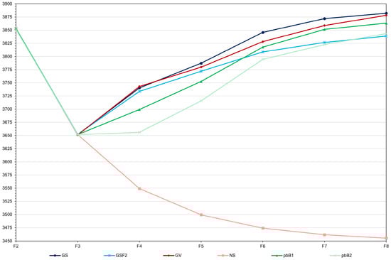
Figure 1.
Average grain yield (kg ha−1) over generations for GS—genomic selection with model updating (average standard deviation (sd) = 17.2), GSF2—genomic selection with no model updating (average sd = 18.6), GV—selection by the true genotypic value (average sd = 12.3), NS—no selection (average sd = 10.7), pbB1—pedigree-based BLUP with full phenotyping (average sd = 22.3), and pbB2—pedigree-based BLUP with partial phenotyping (average sd = 21.0).
There was a marked decrease in the population genotypic variance because of selection, regardless of the selection process (Figure 2). Note that inbreeding decreased the genotypic variance in F8 by approximately 7%. With selection, the decreases ranged from approximately 95 to 100%. Genomic selection caused a more rapid reduction in genotypic variance in the initial cycles (F3−F4) compared to other methods. Fitting exponential models (R2 in the range 0.90 to 1.00), the lowest rate of decrease, from F3, occurred with selection based on the true genotypic value. For the other procedures the rates were similar (−0.85 to −1.05). However, in the long term, all methods resulted in a significant decrease in genetic variability. Regarding the additive value prediction accuracy, in general, except for genomic selection with no model updating, the values observed in F3 to F6 were higher than the accuracy of the phenotypic value, whose selection process assumes phenotyping of all plants (Figure 3). It is important to emphasize that, for the two genomic selection and the two pedigree-based BLUP processes, the correlations between the additive value prediction accuracy and the genetic gain were of high magnitude (0.92 to 0.99). Based on the Least Significant Difference for the F8 progenies (31.9 kg ha−1), genomic selection with model updating provided the progeny with the highest genotypic value (3939.8 kg ha−1). Among the group of 31/500 superior progenies obtained in the 10 simulations, statistically equal to the best progeny, 20 were derived from genomic selection with model updating, nine from selection based on the true genotypic value, and two from pedigree-based BLUP with partial phenotyping (Figure 4). A significant result was that even the top 17% of F8 progenies selected by genomic selection with model updating failed to surpass the genotypic value of the superior parent (3995.4 kg ha−1), being roughly 1–2% suboptimal (Figure 4). This indicates a limitation under the infinitesimal model when parents are far apart.
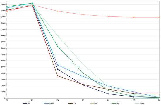
Figure 2.
Average genotypic variances of grain yield ((kg ha−1)2) over generations for GS—genomic selection with model updating (average standard deviation (sd) = 305.5), GSF2—genomic selection with no model updating (average sd = 621.3), GV—selection by the true genotypic value (average sd = 358.0), NS—no selection (average sd = 686.0), pbB1—pedigree-based BLUP with full phenotyping (average sd = 470.7), and pbB2—pedigree-based BLUP with partial phenotyping (average sd = 802.1).
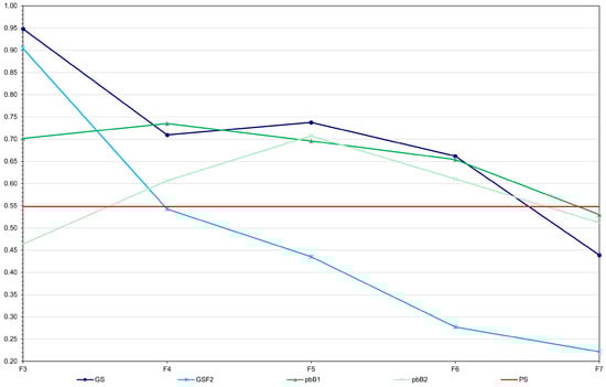
Figure 3.
Average additive value prediction accuracy for grain yield over generations for GS—genomic selection with model updating (average standard deviation (sd) = 0.07), GSF2—genomic selection with no model updating (average sd = 0.06), pbB1—pedigree-based BLUP with full phenotyping (average sd = 0.07), and pbB2—pedigree-based BLUP with partial phenotyping (average sd = 0.09). PS indicates phenotypic selection.
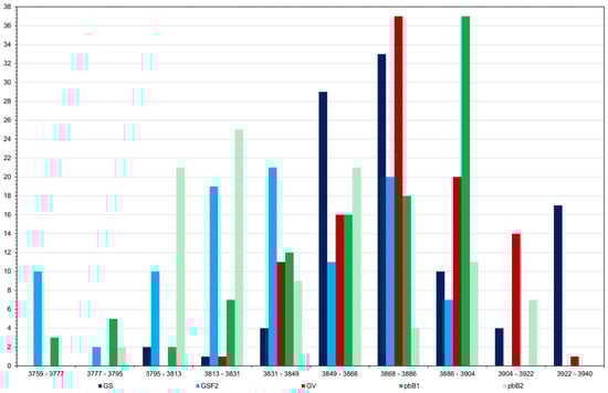
Figure 4.
Frequency distribution of the average genotypic value (kg ha−1) of 100 F8 progenies obtained in the 10 simulations of GS—genomic selection with model updating, GSF2—genomic selection with no model updating, GV—selection by the true genotypic value, pbB1—pedigree-based BLUP with full phenotyping, and pbB2—pedigree-based BLUP with partial phenotyping.
Increasing the selection intensity in F3 led to an increase in the genomic selection efficiency of 5.8% (total gain of 243.7 kg ha−1) (Figure 5). However, the two F8 means were statistically equal (p value of 0.30). Since F2 selection reduced inbreeding depression (3.4 and 2.5 versus 5.2%), the analysis of the F2 selection effect should be based on the F8 genotypic means, as the F3 means are not all comparable. Selecting 50 and 25% of the F2 plants did not change the average yield of the 10 F8 progenies, relative to the genomic selection with model updating (genotypic means of 3881.7 and 3880.2 kg ha−1, respectively). None of the two contrasts were significant (p values of 0.96 and 0.72). Doubling the proportion of selected plants from F3 to F7 resulted in a 14.5% decrease in the genomic selection efficiency (total gain of 197.1 kg ha−1). On the other hand, decreasing by half the proportion of selected plants from F3 to F7 resulted in a 2.6% increase in the genomic selection efficiency (total gain of 236.4 kg ha−1). Only the decrease due to lower selection intensity was statistically significant (p value of 0.004). Increasing the genomic selection intensity did not significantly increase the F8 mean (p value of 0.27). Assuming no dominance resulted in an insignificant increase in the average yield of the F8 progenies (0.3%; p value of 0.30) (Figure 6). The inclusion of 18 QTLs explaining 3.8, 9.4 and 16.8% of the phenotypic variance increased the genomic selection efficiency by 10.7, 38.7 and 82.1%, respectively. Thus, the selection efficiency was proportional to the phenotypic variance explained by the QTLs. The differences between the F8 means relative to the scenario of no QTL were highly significant (p values lower than 1 × 10⁻⁵).
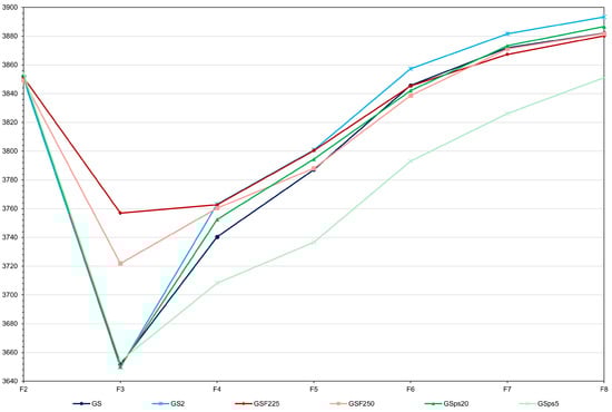
Figure 5.
Average grain yield (kg ha−1) over generations for GS—genomic selection with model updating (average standard deviation (sd) = 16.1), GS2—genomic selection with F2 of size 1000 and F3 of size 10,000 (average sd = 10.0), GSF225 and 50—genomic selection starting in F2, assuming 25 and 50% of selected plants (average sd = 26.7 and 15.1), and GSps5 and 20—genomic selection with high and low selection intensity (average sd = 7.1 and 21.2).
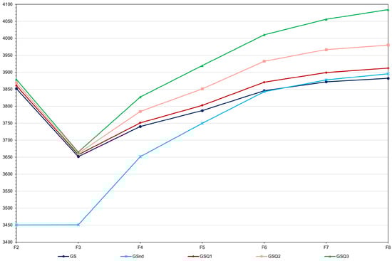
Figure 6.
Average grain yield (kg ha−1) over generations for the scenarios GS—genomic selection with model updating (average standard deviation (sd) = 10.5), GSnd—genomic selection assuming no dominance (average sd = 15.0), and GSQ1, 2 and 3—genomic selection considering 18 QTLs explaining 3.8, 9.4 and 16.8% of the phenotypic variance, respectively (average sd = 11.1, 10.7, and 15.4).
To investigate, under the infinitesimal model, why none selected F8 plant showed genotypic value higher than the superior parent, we assessed the average numbers of homozygous genotypes for the favorable and the unfavorable alleles, and of heterozygous genotypes, in the F2 to F8 generations (Figure 7 and Figure 8). This occurred because of random fixation of the unfavorable alleles in selected heterozygotes. When a selected individual is heterozygous for a gene, the probability of random fixation of the unfavorable allele is 1/4. Note that genomic selection in F2 (in heterozygous loci) increased in 7% the number of homozygous loci for the favorable allele in the F3 plants, relative to the value expected with random fixation (Figure 7). With selection from F3 to F7, the increase was 36% (Figure 8).
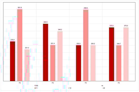
Figure 7.
Average numbers (3 simulations) of genotypes 11, 12 and 22 in the F2 and F3 generations, relative to the 1000 genes controlling grain yield, assuming no selection (ns) and genomic selection of 50% of the F2 plants (50). In this case, the numbers refer to the 500 selected plants. Code 1 identifies the favorable allele.
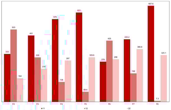
Figure 8.
Average numbers of genotypes 11, 12 and 22, relative to the 1000 genes controlling grain yield, in the five superior F8 progenies derived by genomic selection with model updating and in their F2 to F7 ancestors. Code 1 identifies the favorable allele.
4. Discussion
The genomic selection with model updating provided the highest total realized genetic gain, outperforming the pedigree-based BLUP. We emphasize that this process achieved the same efficiency as selection by the true genotypic value. In other studies based on simulated data, genomic selection was shown to be superior to phenotypic selection, although only in the short and medium term [14] and for some breeding strategies [12]. Tessema, Liu, Sorensen, Andersen and Jensen [15] observed a marked difference between the methods. The genetic gain with genomic selection was three times higher. However, Lin et al. [26] observed no clear differences between the genetic gains/cycle from phenotypic and genomic selection, regardless of selection strategy and initial number of parents. Based on field data, Bandillo, Jarquin, Posadas, Lorenz and Graef [16] concluded that the two methods showed equivalent efficiency. In addition to greater efficiency in terms of genetic gain, the genomic selection with model updating maximized the probability of obtaining F8 progeny with a higher genotypic mean, as also observed in the study of Bandillo, Jarquin, Posadas, Lorenz and Graef [16]. Ignoring selection based on the true genotypic value, 90.9% of the superior F8 progenies were obtained from genomic selection with model updating.
Model updating is recognized as an important factor affecting genomic selection. Restricting the training set for the F2 plants led to a 19% decrease in total genetic gain. But the cost of phenotyping was 86% lower. And phenotyping is expensive. The probability of selecting superior F8 progeny was also reduced. Thus, updating the genomic model by means of partial phenotyping over generations had an impact on genomic selection efficiency. One of the main findings of Chiaravallotti, Lin, Arief, Jahufer, Osorno, McClean, Jarquin and Hoyos-Villegas [12] was that model updating only improved genetic gain in one or two following cycles. Sabadin, DoVale, Platten and Fritsche-Neto [13] concluded that all investigated updating methods led to similar additive values prediction accuracies, whose values were significantly higher than the accuracies with no updating.
Regarding the impact of selection intensity, only in F3 or in all generations, we observed a significant effect on the genetic gains. Decreasing by half the proportion of selected plants only in F3 and in all generations increased the cumulative gain by 5.8 and 6.5%, respectively. However, the decrease in the total gain resulting from doubling the percentages of selected plants was 19%. In other studies, higher selection intensities increased the genomic selection efficiency in early [17] and advanced generations [16]. In our investigation, model updating, selection intensity, and selection strategy were the most important factors affecting the genomic selection efficiency. da Silva, Xavier and Faria [14] observed that breeding strategy had a higher impact on total genetic gain than selection intensity. This concurs with our results, where the change in breeding strategy (e.g., by selection in F2) had minimal effect, but changes in selection intensity from within the core strategy (from F3) had more influence.
Mendonça, Galli, Malone and Fritsche-Neto [17] consider that low-intensity selection in F2 will help to increase the selection efficiency in advanced stages. In contrast, our findings did not yield any advantage. This could be due to variations in the simulated trait architecture, the higher marker density used here, or the exact strategies compared. Due to positive correlations between the predicted additive values of F2 plants and the values of F2:4 progenies, Bonnett et al. [27] concluded that the application of genomic selection in early generations is valid. We also demonstrated that the genomic selection efficiency was not affected by dominance effects. It is worth noting that only additive effects were assumed in most of the simulation-based studies [12,14,15]. In studies with simulated data, it is common to include QTL effects. In our study, the genomic selection efficiency increased proportionally to the phenotypic variance explained by the QTLs, which was also observed by Chiaravallotti, Lin, Arief, Jahufer, Osorno, McClean, Jarquin and Hoyos-Villegas [12]. In that study, the authors observed an increase in the prediction accuracy due to an increase in the QTL number.
In our study, as also observed by Seno et al. [28], although in panmictic populations, pedigree-based BLUP is a genetic evaluation strategy that cannot be disregarded, at least in the development of pure lines. Although this method is inferior to genomic selection in terms of maximizing the probability of selecting superior F8 progeny, the difference in the cumulative gains was 8.2% with full phenotyping and two times higher with partial phenotyping. It is important to emphasize that genomic prediction including genotyped and non-genotyped individuals (single-step genomic-BLUP) has become the prevalent methodology for genetic evaluations in livestock populations [29]. If we assume that the seed company/research institution has the infrastructure of human resources, agricultural equipment, and inputs to carry out phenotypic selection, but depends on third parties for DNA extraction and genotyping, the difference in costs between genomic selection and pedigree-based BLUP with partial phenotyping is the cost of DNA extraction and genotyping. Akdemir and Isidro-Sanchez [30] consider that the high cost of phenotyping is the most important constraint in plant breeding since the genotyping cost has continuously decreased while the phenotyping cost remains constant. Obsteter et al. [31] demonstrated that dairy breeding programs can increase genetic gains by reallocating phenotyping resources into genotyping, regardless of the amount and cost of genotyping. Furthermore, the decrease in the genotyping costs per sample in recent years are making genomic selection more accessible.
Any effective selection process decreases variability. In our study, we observed no differences between the long-term selection processes, as occurred in the studies of Bandillo, Jarquin, Posadas, Lorenz and Graef [16], da Silva, Xavier and Faria [14], and Tessema, Liu, Sorensen, Andersen and Jensen [15]. In these investigations, involving field- and simulated-data, genomic selection led to a higher decrease in the genotypic variance. A significant result from our analysis of the additive value prediction accuracy was a perfect correlation between accuracy and genetic gains, demonstrating the importance of accuracy for predicting the efficiency of a selection process. From F2 to F7, the accuracy of genomic selection decreased from 0.95 to 0.44, indicating a decrease in the selection efficiency due to reduction in the genotypic variance, confirmed by the decrease in the genetic gains. Tessema, Liu, Sorensen, Andersen and Jensen [15] observed increases in accuracy and genetic gain from F6 to F8, associated with a high correlation (0.93). Michel, Löschenberger, Ametz, Pachler, Sparry and Bürstmayr [18] consider that prediction accuracy in initial generations can be increased by combining phenotypic and genomic information.
One additional result needs to be discussed. Note that, assuming the infinitesimal model, when crossing two pure lines with 70 and 30% of the favorable genes and performing genomic selection, the 17/100 F8 progenies with the highest average genotypic values did not outperform the superior parent. This shows that genomic selection failed to provide an elite pure line with much more than 70% of the favorable genes. This is not due to any limitation of this method, but rather to the random fixation of the unfavorable alleles in heterozygous loci of the selected plants. Theoretically, on average, 25% of fixation is expected in F2. Analyzing the genotypes for the 1000 genes, we observed, on average, 250 loci 22 in F2. Two is the code for the unfavorable allele. With 50% selection of F2 plants, there were, on average, 348 loci 22 in F3. This indicates that in this selection cycle, the best pure line could only accumulate 652 loci 11 (9% lower than the superior parent). Considering that there were, on average, 400 loci 11, there were only, on average, 252 heterozygous loci to allow fixation of the favorable allele. However, when a heterozygous plant is selected, the probability of random fixation of the unfavorable allele is 25%.
The analysis of the genotypes of 50 plants in the five F8 progenies with the highest average genotypic values revealed, on average, 325 loci 22 and 7 loci 12, derived from F3 plants with, on average, 230 loci 22 and 309 loci 12. Therefore, even with selection, there was random fixation of (325 − 230)/(309 − 7) = 31.5% of the heterozygous loci in F3. This value is higher than expected without selection (25%), but the superior F8 plants had, on average, 668 loci 11 and, still available for selection, seven loci 12. In other words, selection based on the predicted additive value fixed the favorable allele at (668 − 461)/(309 − 7) = 68.5% − 31.5% (random fixation) = 37% of the loci in heterozygosity in F3. Our analysis reveals that genomic selection is overwhelmingly able to fix superior alleles. The results, however, also reveal a fundamental limitation, under the infinitesimal model: when original parents are vastly divergent, the genetic limit for any derived pure line is restricted. Thus, the potential for going beyond the better parent is greater when crossing parents of higher similarity.
Considering that self-pollinated crop breeders generally do not measure plants, but plot/progenies, that they simultaneously assess progenies from several biparental crosses, and that both genotyping and phenotyping are expensive, integrating genomic selection in pure line breeding is a challenger. We believe that a good alternative for genomic selection would be partial phenotyping and genotyping of F3 plants (to fit the prediction model), genotyping of Fn parents (n > 3), and phenotyping of their Fn+1 progeny. The objective is to predict the Fn plants breeding values using the inbred progeny model [32]. In this case, the choice of plants within the selected progeny would be at random. To minimize the costs of genotyping, the breeder can use low density panel or imputation. For updating the prediction model, the random parents in the selected Fn+1 progeny needs to be phenotyped. In our opinion, however, an increase of 19% in the genomic selection efficacy with model updating does not justify 30% of phenotyping from F4 to F7.
5. Conclusions
Genomic selection with model updating in each cycle maximized the probability of selecting superior F8 progeny and provided the higher total genetic gain, comparable to the selection based on the true genotypic value. Training set size and selection intensity are key factors affecting the development of elite pure lines. Dominance does not significantly affect genomic selection efficiency. The existence of QTLs increases genomic selection efficiency, proportional to the percentage of the phenotypic variance explained by the QTLs. There is no justification for selecting in F2. Pedigree-based BLUP cannot be disregarded as a genetic assessment method in pure line breeding. All selection methods provided a higher decrease in the genotypic variance at F8. The prediction accuracies with genomic selection showed almost perfect correlation with the genetic gains. This work measured a major problem in pure line breeding: random fixation of unfavorable alleles. Our data show that genomic selection is an effective means to counteract this problem. The solution demonstrated here is the application of genomic selection, which effectively maximizes selection for homozygotes for the favorable allele and thereby reduces the undesirable effect of random genetic drift.
Author Contributions
Conceptualization, J.M.S.V.; methodology, J.M.S.V.; software, J.M.S.V.; formal analysis, J.P.A.d.S.; data curation, J.M.S.V.; writing—original draft preparation, J.P.A.d.S.; writing—review and editing, J.M.S.V.; funding acquisition, J.M.S.V. All authors have read and agreed to the published version of the manuscript.
Funding
This research was funded by The National Council for Scientific and Technological Development (CNPq), the Brazilian Federal Agency for Support and Evaluation of Graduate Education (CAPES; Finance Code 001), and the Foundation for Research Support of Minas Gerais State (FAPEMIG).
Data Availability Statement
The dataset is available at https://doi.org/10.6084/m9.figshare.25864315.v2.
Conflicts of Interest
The authors declare no conflicts of interest.
Abbreviations
The following abbreviations are used in this manuscript:
| GS | Genomic selection |
| GV | Selection based on the true genotypic value |
| NS | No selection |
| pbB | Pedigree-based BLUP |
| PS | Phenotypic selection |
References
- Melchinger, A.E.; Fernando, R.; Stricker, C.; Schön, C.C.; Auinger, H.J. Genomic prediction in hybrid breeding: I. Optimizing the training set design. Theor. Appl. Genet. 2023, 136, 176. [Google Scholar] [CrossRef]
- Basnet, B.R.; Crossa, J.; Dreisigacker, S.; Perez-Rodriguez, P.; Manes, Y.; Singh, R.P.; Rosyara, U.R.; Camarillo-Castillo, F.; Murua, M. Hybrid Wheat Prediction Using Genomic, Pedigree, and Environmental Covariables Interaction Models. Plant Genome 2019, 12, 180051. [Google Scholar] [CrossRef]
- Persa, R.; Vieira, C.C.; Rios, E.; Hoyos-Villegas, V.; Messina, C.D.; Runcie, D.; Jarquin, D. Improving predictive ability in sparse testing designs in soybean populations. Front. Genet. 2023, 14, 1269255. [Google Scholar] [CrossRef]
- Ward, B.P.; Brown-Guedira, G.; Tyagi, P.; Kolb, F.L.; Van Sanford, D.A.; Sneller, C.H.; Griffey, C.A. Multienvironment and Multitrait Genomic Selection Models in Unbalanced Early Generation Wheat Yield Trials. Crop Sci. 2019, 59, 491–507. [Google Scholar] [CrossRef]
- Dreisigacker, S.; Perez-Rodriguez, P.; Crespo-Herrera, L.; Bentley, A.R.; Crossa, J. Results from rapid-cycle recurrent genomic selection in spring bread wheat. G3 2023, 13, jkad025. [Google Scholar] [CrossRef] [PubMed]
- Merrick, L.F.; Herr, A.W.; Sandhu, K.S.; Lozada, D.N.; Carter, A.H. Utilizing Genomic Selection for Wheat Population Development and Improvement. Agronomy 2022, 12, 522. [Google Scholar] [CrossRef]
- Chung, P.Y.; Liao, C.T. Selection of parental lines for plant breeding via genomic prediction. Front. Plant Sci. 2022, 13, 934767. [Google Scholar] [CrossRef] [PubMed]
- Chung, P.Y.; Liao, C.T. Identification of superior parental lines for biparental crossing via genomic prediction. PLoS ONE 2020, 15, e0243159. [Google Scholar] [CrossRef]
- Morais, O.P., Jr.; Müller, B.S.F.; Valdisser, P.; Brondani, C.; Vianello, R.P. Genomic prediction for drought tolerance using multienvironment data in a common bean (Phaseolus vulgaris) breeding program. Crop Sci. 2023, 63, 2145–2161. [Google Scholar] [CrossRef]
- Miller, M.J.; Song, Q.J.; Li, Z.L. Genomic selection of soybean (Glycine max) for genetic improvement of yield and seed composition in a breeding context. Plant Genome 2023, 16, e20384. [Google Scholar] [CrossRef]
- Haile, T.A.; Walkowiak, S.; N’Diaye, A.; Clarke, J.M.; Hucl, P.J.; Cuthbert, R.D.; Knox, R.E.; Pozniak, C.J. Genomic prediction of agronomic traits in wheat using different models and cross-validation designs. Theor. Appl. Genet. 2021, 134, 381–398. [Google Scholar] [CrossRef]
- Chiaravallotti, I.; Lin, J.; Arief, V.; Jahufer, Z.; Osorno, J.M.; McClean, P.; Jarquin, D.; Hoyos-Villegas, V. Simulations of multiple breeding strategy scenarios in common bean for assessing genomic selection accuracy and model updating. Plant Genome 2024, 17, e20388. [Google Scholar] [CrossRef]
- Sabadin, F.; DoVale, J.C.; Platten, J.D.; Fritsche-Neto, R. Optimizing self-pollinated crop breeding employing genomic selection: From schemes to updating training sets. Front. Plant Sci. 2022, 13, 935885. [Google Scholar] [CrossRef] [PubMed]
- da Silva, É.; Xavier, A.; Faria, M.V. Impact of Genomic Prediction Model, Selection Intensity, and Breeding Strategy on the Long-Term Genetic Gain and Genetic Erosion in Soybean Breeding. Front. Genet. 2021, 12, 637133. [Google Scholar] [CrossRef] [PubMed]
- Tessema, B.B.; Liu, H.M.; Sorensen, A.C.; Andersen, J.R.; Jensen, J. Strategies Using Genomic Selection to Increase Genetic Gain in Breeding Programs for Wheat. Front. Genet. 2020, 11, 578123. [Google Scholar] [CrossRef]
- Bandillo, N.B.; Jarquin, D.; Posadas, L.G.; Lorenz, A.J.; Graef, G.L. Genomic selection performs as effectively as phenotypic selection for increasing seed yield in soybean. Plant Genome 2023, 16, e20285. [Google Scholar] [CrossRef]
- Mendonça, L.D.; Galli, G.; Malone, G.; Fritsche-Neto, R. Genomic prediction enables early but low-intensity selection in soybean segregating progenies. Crop Sci. 2020, 60, 1346–1361. [Google Scholar] [CrossRef]
- Michel, S.; Löschenberger, F.; Ametz, C.; Pachler, B.; Sparry, E.; Bürstmayr, H. Simultaneous selection for grain yield and protein content in genomics-assisted wheat breeding. Theor. Appl. Genet. 2019, 132, 1745–1760. [Google Scholar] [CrossRef]
- Viana, J.M.S.; Pereira, H.D.; Mundim, G.B.; Piepho, H.P.; Silva, F.F.E. Efficiency of genomic prediction of non-assessed single crosses. Heredity 2018, 120, 283–295. [Google Scholar] [CrossRef] [PubMed]
- Pereira, H.D.; Viana, J.M.S.; Andrade, A.C.B.; Silva, F.F.E.; Paes, G.P. Relevance of genetic relationship in GWAS and genomic prediction. J. Appl. Genet. 2018, 59, 1–8. [Google Scholar] [CrossRef]
- Viana, J.M.S.; Souza, C.A.S. Efficiency of mapping epistatic quantitative trait loci. Heredity 2023, 131, 25–32. [Google Scholar] [CrossRef]
- VanRaden, P.M. Efficient methods to compute genomic predictions. J. Dairy Sci. 2008, 91, 4414–4423. [Google Scholar] [CrossRef]
- Amadeu, R.R.; Cellon, C.; Olmstead, J.W.; Garcia, A.A.; Resende, M.F.; Munoz, P.R. AGHmatrix: R Package to Construct Relationship Matrices for Autotetraploid and Diploid Species: A Blueberry Example. Plant Genome 2016, 9, plantgenome2016.01.0009. [Google Scholar] [CrossRef] [PubMed]
- Cockerham, C.C. Covariances of relatives from self-fertilization. Crop Sci. 1983, 23, 1177–1180. [Google Scholar] [CrossRef]
- Endelman, J.B. Ridge regression and other kernels for genomic selection with R package rrBLUP. Plant Genome 2011, 4, 250–255. [Google Scholar] [CrossRef]
- Lin, J.; Arief, V.; Jahufer, Z.; Osorno, J.; McClean, P.; Jarquin, D.; Hoyos-Villegas, V. Simulations of rate of genetic gain in dry bean breeding programs. TAG. Theor. Appl. genetics. Theor. Und Angew. Genet. 2023, 136, 14. [Google Scholar] [CrossRef]
- Bonnett, D.; Li, Y.; Crossa, J.; Dreisigacker, S.; Basnet, B.; Perez-Rodriguez, P.; Alvarado, G.; Jannink, J.L.; Poland, J.; Sorrells, M. Response to Early Generation Genomic Selection for Yield in Wheat. Front. Plant Sci. 2021, 12, 718611. [Google Scholar] [CrossRef]
- Seno, L.D.; Guidolin, D.G.F.; Aspilcueta-Borquis, R.R.; do Nascimento, G.B.; da Silva, T.B.R.; de Oliveira, H.N.; Munari, D.P. Genomic selection in dairy cattle simulated populations. J. Dairy Res. 2018, 85, 125–132. [Google Scholar] [CrossRef]
- Bermann, M.; Cesarani, A.; Misztal, I.; Lourenco, D. Past, present, and future developments in single-step genomic models. Ital. J. Anim. Sci. 2022, 21, 673–685. [Google Scholar] [CrossRef]
- Akdemir, D.; Isidro-Sanchez, J. Design of training populations for selective phenotyping in genomic prediction. Sci. Rep. 2019, 9, 1446. [Google Scholar] [CrossRef]
- Obsteter, J.; Jenko, J.; Gorjanc, G. Genomic Selection for Any Dairy Breeding Program via Optimized Investment in Phenotyping and Genotyping. Front. Genet. 2021, 12, 637017. [Google Scholar] [CrossRef] [PubMed]
- Viana, J.M.S.; Faria, V.R.; Fonseca e Silva, F.; Vilela de Resende, M.D. Best Linear Unbiased Prediction and Family Selection in Crop Species. Crop Sci. 2011, 51, 2371–2381. [Google Scholar] [CrossRef]
Disclaimer/Publisher’s Note: The statements, opinions and data contained in all publications are solely those of the individual author(s) and contributor(s) and not of MDPI and/or the editor(s). MDPI and/or the editor(s) disclaim responsibility for any injury to people or property resulting from any ideas, methods, instructions or products referred to in the content. |
© 2025 by the authors. Licensee MDPI, Basel, Switzerland. This article is an open access article distributed under the terms and conditions of the Creative Commons Attribution (CC BY) license (https://creativecommons.org/licenses/by/4.0/).