Abstract
Uncertainties continue to prevail in the potential of natural forests and plantations in carbon stock assessment. The present study was carried out to assess the carbon stock in natural and plantation forests of Manipur using geo-informatics in Imphal East and West districts. The integrated approach of geospatial technology, along with field inventory based data, was used in spatial modeling of biomass carbon of selected natural and plantation forests. The stand density was similar for both LNG and TRS forests (680 individuals ha−1) and lowest for KHP forest (640 individuals ha−1). Paulownia fortunei (770 individuals ha−1) showed highest density among tree species while Tectona grandis (54.07 m2 ha−1) followed by Gmelina arborea (42.18 m2 ha−1) had higher basal area compared to other tree species. The soil moisture content (%) in the natural forest ranged from 19.13 ± 0.47 to 26.9 ± 0.26%. The soil moisture content in the plantation forest ranged from 19.16 ± 0.98 to 25.83 ± 0.06%. The bulk density of natural forests ranged from 1.27 g cm−3 to 1.37 g cm−3 while for plantation forests it ranged from 1.18 g cm−3 to 1.34 g cm−3. Among the studied sites of natural forest, TRS forest had both the highest AGBC value of 132.74 t ha−1 as well as the BGBC value of 38.49 t ha−1. Similarly, among the plantations, T. grandis plantation showed the highest AGBC (193 t ha−1) and BGBC (55.97 t ha−1). On the other hand, Tharosibi forest and T. grandis plantation had the highest total carbon stock for natural and plantation forest with values of 274.824 t ha−1 and 390.88 t ha−1, respectively. The total above-ground carbon stock estimated for the natural forest of KHP, LNG and TRS were 109.60 t ha−1, 79.49 t ha−1 and 132.74 t ha−1, respectively. On the other hand, the estimated total above-ground carbon stock in plantation of GA, PD, PF and TG were 62.93 t ha−1 62.81 t ha−1, 45.85 t ha−1 and 193.82 t ha−1. In the present study, the relationship with the biomass was observed to be better in SAVI compared to NDVI and TVI. The linear regression analysis performed to determine the relationship between the estimated and predicted biomass resulted in a correlation coefficient of R2 = 0.85 for the present study area, which is an indication of a good relationship between the estimated and predicted biomass.
1. Introduction
The terrestrial ecosystem acts as a spatially and temporally variant carbon source and sink due to its monsoon-grounded climate system, diversified land use and land cover distribution and cultural practices. Human-induced change in land-use practices has been considered as foremost driver for alteration persuading the Earth’s ecosystem and climate [1]. According to 5th report Assessment of the Intergovernmental Panel on Climate Change (IPCC), deforestation is explicitly regarded as the second largest source of carbon dioxide (CO2) emission after the emission from fossil fuel burning [2]. The deforestation and land-use change combined caused emission of around 1.0 Pg C per year in tropical regions [3]. Hence, the atmospheric CO2 concentration reduction has been recognized as a major agenda among the nations under the Kyoto Protocol and the Paris Agreement [4].
As an integral part of terrestrial ecosystem, the natural forest has a noteworthy contribution in earth’s energy cycle and is regarded as the largest storehouse of terrestrial ecosystem carbon. The forest stores carbon in the form biomass in its different body parts known as carbon pool [5]. Among the different pools, the above-ground biomass (AGB) pool has been considered as a crucial indicator of many forest ecosystem processes [6]. Undisturbed forest ecosystems or natural forests are generally highly productive and accumulate more biomass and carbon per unit area compared to other land use systems such as agriculture and plantation forests. Forest plantations also have a significant role on the global carbon sink [7,8,9].
Many researchers reported that soil holds around 2344 Gt organic carbon and a little disturbance to the soil organic carbon pool could result in significant effects on the atmospheric carbon dioxide (CO2) concentration [10]. According to Lal [11], by increasing the input of C into soil compared to output through good soil management practices could enhance soil organic carbon (SOC) sequestration while higher output causes loss of carbon into the atmosphere.
To address the regional carbon stock and carbon sequestration potential of forest ecosystem, it is ultimately necessary to assess the forest biomass of the region. Researchers around the globe have used three major approaches such as field-based measurements, integrated approach of field inventory and satellite-based data, and the process-based ecosystem model [12,13]. Among the available methods of biomass assessment, direct measurement is the traditional way of measurement and the most accurate; however, it is laborious and costly. The remote-sensing-based approach has now become the most widely accepted method of biomass assessment due to its spatial, spectral and temporal advantages over the traditional measurements, to address issues such as large areal coverage, complex forest landscape, biomass assessment at different scale, long-term, real-time monitoring of AGB [14,15]. Satellite data from NOAA (National Oceanic and Atmospheric Administration), SPOT (French: Satellite Pour l’Observation de la Terre, (Satellite for Observation of Earth), LANDSAT, IKONOS, etc. have enormous potential in assessing terrestrial biomass and carbon pools. Recently many researchers have used this satellite data for AGB and carbon estimation. It uses spectral reflectance properties of the satellite data as these contained an integrated effect of forest canopy through factors such as vegetation composition, soil characteristics, atmospheric condition and topographic effect [16]. Devagiri et al. [17] estimated the AGB and carbon pool in different vegetation types of the south western part of Karnataka using field-based and spectral modeling. Baishya et al. [18] reported a comparative analysis of above-ground biomass in Sal plantation and natural forests of north east India. Many researchers have used the spectral vegetation indices (VI) model for estimating the biomass [17,19,20,21].
There are basically two approaches to estimate above-ground biomass (ABG) carbon. These can be destructive—by cutting down the trees and woody components, developing a model biomass [22,23,24]—or a non-destructive remote-sensing approach [25,26,27]. The complex association of forest tree species principally limits direct harvesting in multi-species stands [28], besides, the destructive approach being very costly, time-consuming and non environmentally friendly, remote sensing is being mostly used by the researchers during recent years. Changes due to anthropogenic land use and land cover is the most important threat to biodiversity and ecosystems the world over [29,30,31,32]. Therefore, efforts are constantly being carried out to estimate the carbon stock and sequestration potential of different forest types (both locally and regionally) so that due conservation efforts could be made [33]. Correct protocols are highly recommended for assessment of carbon stock in forested landscapes [34]. In the remote sensing approach, selection of appropriate algorithms to model AGB will play a vital role [35,36,37,38]. There is a conspicuous lack of assessment of carbon stock and sequestration potential of both natural and planted forests of Manipur, a state in northeast India.
The present study aims to estimate and predict the biomass, carbon stock, and sequestration potential of both natural forests and plantations through spatial modeling. It also briefly describes the current scenario of carbon stock in the study area using forest-based data and relates it to plot-based results.
2. Materials and Methods
2.1. Study Area
The state of Manipur is known as “The Land of Jewel” and it is also known for its resource richness, supporting diversity of endemic flora and fauna. It lies within 23°50′ N to 25°42′ N latitudes and 92°59′ E to 94°46′ E longitudes covering a geographical area of 22,327 km2 [39]. The state also lies within the junction of two biodiversity hotspots i.e., ‘The Indo–Myanmar hotspot’ and ‘The Himalayan hotspot’. The recorded area under forest cover is approximately 16,846.90 km2 which is 75.46% of the state’s geographical area [39]. Legally, the forest area distribution is 8.42% under reserved forest, 23.94% under protected forest and 67.64% under unclassed forest [39]. Imphal East district has a geographical area of 709 km2 and forest cover of 274.26 km2. On the other hand, the total geographical area of Imphal West is 519 km2 and the total forest cover is 51.75 km2, respectively (Figure 1). The study area experiences tropical climate with mean annual minimum and maximum temperature of 16 °C and 26.83 °C (Figure 2). The average rainfall and relative humidity of the study sites were 144.79 mm and 74.12%, respectively. The study was carried out in three (3) sites of natural forests i.e., Langol, Khonghampat and Tharosibi forests and four (4) Plantation sites i.e., Gmelina arborea, Populus deltoides, Paulownia fortunei and Tectona grandis.
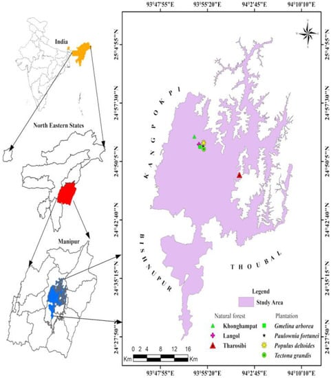
Figure 1.
Selected study area of natural forests and plantations of Imphal East and West districts of Manipur.
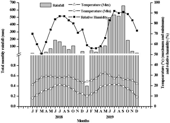
Figure 2.
Climatogram of the study area of natural forests and plantations of Imphal, Manipur.
2.2. Data Base and Methods
2.2.1. Field Measurement
The study was carried out in two selected land use types i.e., natural forests and plantation forests under the Imphal East and West districts of Manipur. For each forest/plantation, three stands each measuring 250 m × 250 m were selected, and at each stand a total of 20 quadrats measuring 10 m × 10 m each were laid randomly for studying community characteristics. All the trees (≥30 cm gbh) enclosed within the quadrats were recorded along with their height and diameter. Community characteristics such as stand density, basal area, mean tree diameter at breast height and mean tree height of the natural forests and plantations were determined according to Misra [40]. Tree individuals with more than 30 cm girth were considered to calculate the AGB for each woody species. Field measuring tape was used to determine the girth of individual trees at breast height i.e., 1.37 m from the base of tree and a Ravi altimeter was used to determine the height of each tree. The data compiled were used for estimation of volume using species-specific equation, considering the physiographic zone of each species following the Forest Survey of India [28]. The given Equation (1) was used to determine the volume of tree species in the study area.
where, D = diameter at 1.37 m i.e., breast height level.
V = 0.11079 − 1.81103 × D + 11.4132 × D2 + 0.38528 × D3
Tree/plant biomass was determined by multiplying the volume with the specific gravity of each individual species. For those species whose specific gravity is not available, the specific gravity value of 0.5 for tropical region [41] was used in the current study. Equation (2) gives the calculation of biomass from volume of tree species.
Biomass = Volume × Specific gravity of the species
The above-ground biomass (AGB) carbon was estimated by assuming that the carbon content is 55% of the total above-ground biomass [42]. By multiplying the factor 0.29 to the AGB value, the corresponding below-ground biomass (BGB) was also calculated.
2.2.2. Remote Sensed Data
The precision of spatial data is important for the user and is essential in the evaluation of the equality of the results of data processing. Landsat OLI optical remote-sensing data sets and ASTER elevation data sets of 2016 were used for the study (Table 1) which were downloaded during January and February, 2020 from Earth Explorer (https://earthexplorer.usgs.gov) [43], a public domain of NASA. The cloud free images were selected and red, green, blue and NIR bands were included in the analysis. All the images were georeferenced to the common UTM (Universal Transversal Mercator) projection with WGS 84 datum (Zone 46). The images were converted to top of atmospheric (TOA) reflectance by radiometric correction method as per Landsat 8 user handbook.

Table 1.
Landsat satellite data used for the present study.
2.2.3. Vegetation Indices
Landsat OLI-derived vegetation indices such as the normalized difference vegetation index (NDVI), soil-adjusted vegetation index (SAVI) and transformed vegetation index (TVI), were used in the present study (Table 2). The tested vegetation indices consist of the NDVI, which is the ratio of contrasting reflectance between the maximum absorption of the red wavelength and maximum reflectance of the infrared wavelength [30]. The SAVI is similar to the NDVI but it adjusts the soil brightness correction factor [31,32]. EVI involves three band ratios which is sensitive to high AGB and also eliminates the atmospheric influence along with the canopy background effect.
Table 2.
Different vegetation indices used.
2.2.4. Regression Analysis between Different Vegetation Indices and Plot Based Biomass
Satellite-derived vegetation indices NDVI, TVI and SAVI were applied to the image of the study area. Based on the location of sample plot, values of the vegetation indices are extracted for each plot. An individual linear regression model was applied to extracted vegetation indices value vs. AGB (t ha−1) based on field inventory data [47].
2.2.5. Spectral Biomass Modelling
A multiple regression approach was used for modelling of spatial biomass and carbon stock. First, an individual tree linear regression analysis model was used to derive the relationship between calculated plot-based biomass and the corresponding different vegetation indices. The resultant best fit model having R2 values were further used for spectral modelling of the biomass and carbon stock for the study area.
2.2.6. Soil Analysis
Within each sampled plot, soil samples were collected systematically at two depths (i.e., 0–15 cm and 15–30 cm) using a metallic soil auger (40 cm deep, 8 cm dia.) at random locations for analysis of various soil parameters. A total of 54 soil samples (3 cores × 2 depths × 3 subplots × 3 major plots) were collected from each studied natural/plantation forests. Soil pH was measured using a pH meter, and soil texture class was identified following the ISSS soil mixture classification system. Soil cores were oven-dried at 105 °C for 48 h to determine soil moisture content gravimetrically. Soil bulk density was determined as the ratio of oven-dried soil mass and the core volume. Soil organic carbon was determined by the rapid dichromate oxidation method [48].
2.2.7. Statistical Analysis
All basic analyses were performed using Microsoft Excel 2010 (Microsoft 2010, USA). Mean and standard errors were calculated using descriptive statistical tools. One-way analysis of variance (ANOVA) and significance of difference at p < 0.05 was detected using the Tukey honest significance (HSD) test. Linear regression was used to estimate biomass from NDVI, TVI and SAVI values using leave-one-out procedure [49]. The predicted biomass was then compared with that measured in the field.
3. Results
3.1. Community Characteristics
Among the natural forests, the trees of the Tharosibi forests had the highest mean height (17.07 m) and average diameter (33.76 cm) and highest stand basal area (71.92 m2 ha−1), respectively (Table 3). However, the stand density was highest for both the Langol and Tharosibi forests (680 individuals ha−1) and lowest in the Khonghampat forest (640 individuals ha−1). On the other hand, among the plantations, the mean height was highest in Populus deltoides (19.09 m) and mean diameter the highest in Tectona grandis (31.63 m). The stand density was highest in Paulownia fortunei (770 individuals ha−1) and the stand basal area the highest in Tectona grandis (54.07 m2 ha−1) followed by Gmelina arborea (42.18 m2 ha−1).
Table 3.
Community characteristics of the selected natural forests and plantations of Imphal East and West districts of Manipur.
3.2. Soil Parameters
The soil moisture content in the natural forest ranged from 19.43 ± 0.43% to 26.9 ± 0.26% in the surface layer whereas it ranged from 19.13 ± 0.47 to 25.46 ± 0.2 in the sub-surface layer (Table 4). The soil moisture content in the plantation forest ranged from 21.2 ± 0.15% to 25.83 ± 0.07% in the surface layer and in the sub-surface layer ranged from 19.16 ± 0.98% to 24.56 ± 1.46% (Table 5). The bulk density in the surface layer of natural forests ranged from 1.35 g cm−3 to 1.37 g cm−3 whereas it ranged from 1.27 g cm−3 to 1.32 g cm−3 in the sub-surface layer (Table 4). The bulk density in the plantation forests ranged from 1.23 g cm−3 to 1.34 g cm−3 in the surface layer whereas it ranged from 1.18 g cm3 to 1.34 g cm−3 in the sub-surface layer (Table 5). The soil texture of the natural forest was sandy loam to sandy clay loam and in the plantation forest it was sandy loam (Table 4 and Table 5). The pH of the soil in the KHP natural forest was found to be more acidic (4.79 ± 0.003) followed by (4.85 ± 0.03) and 5.53 ± 0 in the upper depth of TRS and LNG, respectively (Table 4). The pH in the surface layer of the GA plantation forest (5.41 ± 0.01) was found to be more acidic than the TG (5.583 ± 0.003), PF (5.86 ± 0.01) and PD (6.13 ± 0.01) plantation forest (Table 5). The organic carbon in the natural forests ranged from 102.64 ± 1.35 t ha−1 to 187.64 ± 0.77 t ha−1 in the surface layer and in the sub-surface layer it ranged from 93.82 ± 0.38 t ha−1 to 137.92 ± 2.31 t ha−1 (Table 4). The organic carbon in the plantation forest ranged from 160.38 ± 0 t ha−1 to 181.23 ± 1.60 t ha−1 in the surface layer and in the sub-surface layer it ranged from 115.47 ± 3.20 t ha−1 to 128.3 ± 8.01 t ha−1 (Table 5). The soil organic carbon was found to be highest in the surface soil and it decreased with increase in depth. The organic matter content in the natural forests ranged from 176.95 ± 2.32 t ha−1 to 323.49 ± 1.32 t ha−1 in the surface layer and it ranged from 161.75 ± 0.66 t ha−1 to 237.78 ± 3.98 t ha−1 in the sub-surface layer (Table 4). The organic matter content in the plantation followed the same trend as the soil organic carbon content.
Table 4.
Soil physico-chemical properties at different soil depth in selected natural forests of Imphal East and West districts of Manipur.
Table 5.
Soil physico-chemical properties at different soil depth in selected plantation forests of Imphal East and West districts of Manipur.
3.3. Carbon Stock in Different Pools
Among the study sites of natural forests, Tharosibi forest had the highest AGBC value of 132.74 t ha−1 as well as the highest BGBC value of 38.494 t ha−1. However, the highest soil carbon was recorded in the Langol forest (162.78 t ha−1) and the highest litter carbon was obtained from the Khonghampat forest (3.91 t ha−1). Similarly, among the plantations, the highest AGBC (193 t ha −1) and BGBC (55.97 t ha−1) were both recorded from T. grandis plantation. The highest soil carbon was recorded from P. fortunei (153.56 t ha−1) (Figure 3) and the highest litter carbon was obtained from P. deltoides (1.28 t ha−1), respectively. The Tharosibi forest and T. grandis plantation had the highest total carbon stocks for natural and plantation forests, with values of 274.824 t ha−1 and 390.88 t ha−1, respectively.
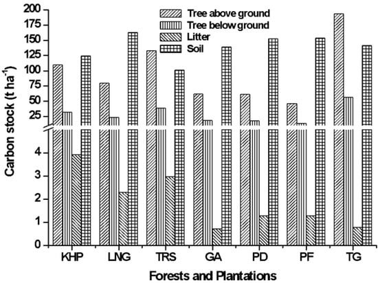
Figure 3.
Carbon stock (t ha−1) in different pools of the in selected natural forests and plantations of Imphal East and West district of Manipur (KHP: Khonghampat, LNG: Langol, TRS: Tharosibi, GA: Gmelina arborea, PD: Populus deltoides, PF: Paulownia fortunei, TG: Tectona grandis).
3.4. Above Ground Biomass and Carbon Estimation Using GIS
The estimated total above-ground biomass from the field-based data for the natural forests of KHP, LNG and TRS were 199.28 t ha−1, 144.53 t ha−1 and 241.34 t ha−1, respectively. Similarly, the total above-ground biomass estimated in plantations of GA, PD, PF and TG were 114.42 t ha−1, 114.20 t ha−1, 83.37 t ha−1 and 352.39 t ha−1, respectively (Table 6). The maximum total AGB (352.39 t ha−1) was recorded in TG plantation. The total above-ground carbon stock estimated for the natural forest of KHP, LNG and TRS were 109.60 t ha−1, 79.49 t ha−1 and 132.74 t ha−1, respectively. On the other hand, the estimated total above-ground carbon stock in plantation of GA, PD, PF and TG were 62.93 t ha−1 62.81 t ha−1 45.85 t ha−1 and 193.82 t ha−1, respectively.
Table 6.
Estimated above-ground biomass and carbon stock in natural forests and plantations.
3.5. Regression Analysis between Different Vegetation Indices and Plot Based Biomass
3.5.1. NDVI
The Landsat-derived normalized difference vegetation index (NDVI) has been carried out by applying it to the image of study area. The NDVI values varied across the study area and it also varied from plantation to plantation. The results showed that the value of NDVI ranged between −0.35 and 0.72. The plot-wise NDVI ranged from 0.35 to 0.52 for KHP, 0.37 to 0.52 for LNG and 0.41 to 0.52 for TRS of natural forest. Similarly, for plantation, the NDVI value ranged from 0.38 to 0.44, 0.35 to 0.48, 0.38 to 0.43 and 0.45 to 0.54 for GA, PD, PF and TG, respectively (Table 7). When a linear regression model was applied to the extracted values of NDVI and between biomass (t ha−1), the resultant correlation coefficient value was (R2 = 0.62). An NDVI map of study area of different season is presented in Figure 4a.
Table 7.
TVI, NDVI, and SAVI values for each sample plot.
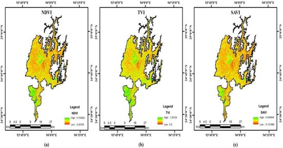
Figure 4.
Vegetation indices map of the study area. (a) NDVI, (b) TVI and (c) SAVI.
3.5.2. TVI
The operation of transformed vegetation index (TVI) was carried out by applying it to the image of the present study area. The TVI values varied across the study area and also varied from different study sites of natural forest as well as from one plantation to another. The present study showed that the value of TVI ranged from 0.5 to 1.35. The plot-wise TVI ranges from 1.09 to 1.22, 1.12 to 1.22 and 1.11 to 1.22 for KHP, LNG and TRS, respectively. Similarly, for plantation, the value ranged from 1.08 to 1.16, 1.09 to 1.19, 0.11 to 0.16 and 0.17 to 1.23 for GA, PD, PF and TG, respectively (Table 7). When linear regression model was applied to the extracted values of TVI and between types of biomass, the resultant correlation coefficient values was (R2 = 0.49). TVI map of study area of different season is presented in Figure 4b.
3.5.3. SAVI
The SAVI was also being performed for the present study area. One of the advantages of the SAVI is that it minimized the soil background effect in the study area and results in better vegetation index value than the NDVI and DVI. In the present study it showed that SAVI value ranged from −0.13 to 0.54. The plot-wise SAVI value ranged from 0.18 to 0.29, 0.19 to 0.26, 0.19 to 0.31 for the natural forest of KHP, LNG and TRS, respectively. On the other hand, the SAVI value in plantation of GA, PD, PF and TG were 0.20 to 0.23, 0.20 to 0.26, 0.19 to 0.23 and 0.26 to 0.34, respectively (Table 7). When linear regression model was applied to the extracted values of SAVI and between types of biomass, the resultant correlation coefficient value was (R2 = 0.62). SAVI map of study area of a different season is presented in Figure 4c.
The coefficient (R2) of regression model biomass and different vegetation indices are given in Table 8.
Table 8.
Coefficient for R2 for biomass and different vegetation indices.
3.6. Spatial Biomass Carbon Prediction through Modeling
The multiple regression modelling used the two best models viz., NDVI and SAVI derived from linear regression analysis of different vegetation indices, and field-based biomass (Figure 5). The regression equation derived (AGB = 96.855 × NDVI + 271.412 × SAVI−116.604 × TVI + 43.47, R2 = 0.84) was used for above-ground biomass prediction. The predicted biomass carbon for the study area was 126.61 t ha−1 (Figure 6). The observed biomass carbon for the natural forests of KHP, LNG and TRS were 141.39 t ha−1, 102.54 t ha−1 and 171.23 t ha−1, respectively. Similarly, the observed biomass carbon in plantations of GA, PD, PF and TG were 81.18 t ha−1, 81.02 t ha−1, 59.15 t ha−1 and 250.02 t ha−1, respectively. However, the predicted biomass from field-based data were 182.11 t ha−1, 122.15 t ha−1, 146.50 t ha−1, 76.55 t ha−1, 89.80 t ha−1, 46.90 t ha−1 and 222.23 t ha−1 for KHP, LNG, TRS, GA, PD, PF and TG, respectively (Table 9). The total biomass carbon stock was predicted by combining AGBC and BGBC (0.29 fraction of AGBC) of the different sites.
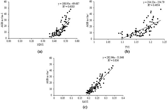
Figure 5.
Linear regression model. (a) NDVI and biomass (t ha−1), (b) TVI and biomass (t ha−1), and (c) SAVI and biomass (t ha−1).
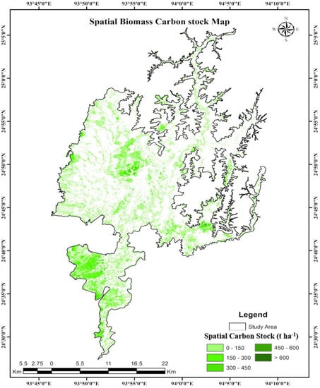
Figure 6.
Spatial carbon stock in the study area of Manipur.
Table 9.
Predicted biomass carbon for different natural forests and plantations.
3.7. The Relationship between Estimated and Predicted Biomass
The correlation coefficient of R2 = 0.8491 was observed for the present study area, which is an indication of good relationship between the estimated and predicted biomass (Figure 7).
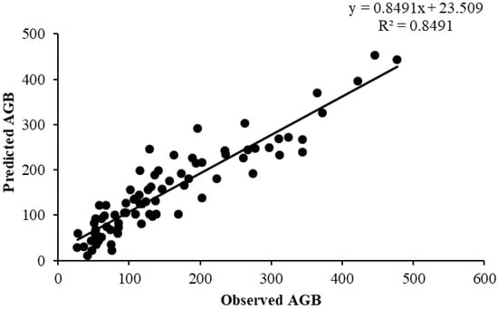
Figure 7.
Linear regression analysis between the observed and predicted biomass.
4. Discussion
4.1. Community Characteristics and Carbon Stocks
Natural forests are found to be typically more diverse with a greater variety of tree species than plantation forests [50]. The variations in basal area of the selected forest stands were related to the number of individual trees of larger girths and diversity of tree species. In the present study, stand density, basal area and mean tree height were the determining factors contributing to forest biomass and above-ground carbon stocks. The above-ground biomass carbon in the present study is comparable with various studies reported in the region [18,51,52,53]. Higher species richness combined with tree size and growth pattern influence various carbon pools of an ecosystem [54,55,56,57]. Among the plantations, T. grandis had higher above-ground biomass owing to their higher mean dbh over other plantations. Highest soil C in P. fortunei and litter C in P. deltoides forests may be due to slower C turnover in these pools. Carbon balance in any pool is governed by both C storage and C loss mediated by several complex processes operating in an ecosystem [55,58,59]. The climatic conditions, vegetative cover and management practices are some of the most important factors that affect the C storage in different pools (live biomass, litter, deadwood and soil). Under the current threat of climate change, it is therefore of paramount importance to properly manage the natural and plantation forests of the region to enhance soil quality, in order to sustain soil health and improve carbon stocks [53].
4.2. Soil Parameters
The maximum percentage of moisture in the surface layer might be due to the higher accumulation of litter on the forest floor [60,61]. The decrease in moisture content with increase in depth could be attributed to the reduced surface evaporation coupled with accumulation of litter and their deposition in the sub-surface layers with specific micro climatic conditions of the area. The variations in the bulk density were attributed to the organic matter content in the soil which accelerates the decomposition rate in the soil [62]. It was found that the pH values decreased with increase in depth. The differences in the soil pH might be due to the dynamic nature of soil organic matter content that releases hydrogen ions which are associated with organic ions by nitrification [63]. Acidity could also be associated with a high possibility of aluminum and other heavy-metal toxicity [64] and leaching of bases under prevailing heavy rainfall and the undulating topography of the area. Fuji [65] also reported that trees and shrubs plays an important role in minimizing soil acidification through the development of deep root systems capable of taking up bases such as Ca and Mg from deep layers of the soil profile and returning them to the topsoil as leaf litter containing excess basic or alkaline cations [58]. The variations in the SOC might be due to the accumulation of organic matter in the forest floor after decomposition of litter [38,39]. The presence of a large amount of dead root material on the soil surface layer greatly enhances the populations of micro-organisms and hence the organic carbon content. The soil organic carbon (SOC) can be extremely regulated by land use and physiographic conditions, particularly altitude and slope. Altitudinal gradients often influence the soil organic carbon content by differences in species composition and factors such as soil pH, soil moisture content, soil texture etc. [66] and it is necessary in regulating the global C cycle [67,68]. Poor soil management and the replacement of native forests by agricultural land may compromise soil health. The dramatic changes in vegetation cover are expected to modify soil C content and nutrient cycling, thus impacting environmental equilibrium and sustainability [69]. The differences in SOC content in the different natural/plantation forests in the present study might be due to differential residue additions that can augment soil aggregation [70], and affect soil profile [71]. The higher SOC content in the forests might be due to its higher tree density, low disturbance in comparison to the other selected land use systems.
4.3. Regression Analysis between Vegetation Indices and Plot-Based Biomss
The correlation coefficient R2 value for NDVI was 0.62. The R2 value for TVI and SAVI were 0.49 and 0. 84, respectively. Devagiri [17] reported an R2 value of 0.73 for rubber plantations, which is higher than in the present study. Ye et al. [72] also reported an R2 value of 0.8519 for AGB. In the present study, the relationship with biomass was observed to be better in SAVI as compared to other indices such as NDVI and TVI. This was due to the fact that SAVI considers the soil brightness factor and minimized it in the resultant images. The model was derived by using data from forest inventory and satellite-based VIs. From the current study it was found that among the selected VIs, the NDVI for AGB estimation and prediction was also used for comparing the results obtained with other indices. It resulted a positive correlation with AGB (R2 = 0.64) but areas with high AGB stock had a severe color intensity and purity problem. It was reported that the saturation could be mainly due to high reflectance in NIR as compared to low reflectance in the red band, which could be responsible for poor correlation [73]. Further, NDVI was more influenced by canopy, optical and geometrical orientation effects due to sun and sensor viewing angle [74]. The SAVI outperformed all other indices. The reason for better performance might be due to inclusion of unique soil adjustment factors, which minimize the soil brightness factor and, as an improvised form, enriched the vegetation mapping and AGB estimation [75,76]. The SAVI performance (R2 = 0.84) in AGB estimation can be compared with the result (R2 = 0.85) reported by others [77,78,79].
To predict the spatial AGB and carbon stock of the study area, a multi-linear regression analysis was utilized in the present study. From the regression analysis it was observed that SAVI (R2 = 0.84) has a better correlation compared to the NDVI (0.62) and TVI (0.49). Among the indices, the SAVI and NDVI have good correlation with the field-based AGB as these two indices have shown a higher R2 value. Further integrating the SAVI and NDVI as a predictor, the subsequent regression model to predict spatial distribution of AGB and carbon stock resulted in better AGB estimation (R2 = 0.85, RMSE) compared to using individual indices as the predictor in regression. The R2 value obtained in the present study can be compared with the value reported using Landsat data [80,81].
4.4. Spatial Biomass C Prediction through Modeling
The spatial AGB predicted for the natural forest was 122.15 to 182.11 t ha−1 with a mean AGB of 150.25 t ha−1 and the values can be compared with those of other researchers who used the Landsat OLI for their studies [82,83]. Thumaty et al. [83] have reported a smaller AGB of 58 t ha−1 for the deciduous forests of India. However, the present research’s AGB was found to be lower compared to the AGB (230 t ha−1) value reported from the evergreen forest of Karnataka [17] and mangrove forest (250.53 t ha−1) of Thailand [84]. Similarly, the AGB predicted for the plantation forest (108.87 t ha−1) can be compared with that reported from the Kodagu teak plantation (118.19 t ha−1) by Devagiri et al. [17] and the 196.2 t ha−1 in a plantation forest in Arunachal Pradesh [85,86], while it was lower than AGB reported from a plantation forest of Papum Pare district of Arunachal Pradesh [87].
5. Conclusions
From the present study, it is found that tree-based systems (forests and plantations) are important carbon sinks, and have the potential to mitigate climate change. The ability of these systems to store carbon depends on species composition, tree age and size, and the soil’s physico-chemical properties and climatic conditions. These systems therefore may be sustainably managed to preserve ecological integrity, and deliver sustainable development goals (SDG 13), and contribute to the nationally determined contributions of the United Nations Framework Convention on Climate Change. This study also explored the potential of optical remote sensing data (Landsat OLI) for the prediction of the spatial biomass density and carbon sequestration of the selected plantations. This study revealed that the SAVI was the most suitable vegetation index as it has a strong relationship with the estimated AGB of plantations. Hence, it is suggested that SAVI may be used for the estimation of AGB in plantations in other parts of the country.
Author Contributions
Conceptualization: H.W. and O.P.T. Supervision: O.P.T. Writing—original draft: H.W., A.P., R.B., B.D. and O.P.T. Review: editing and finalization: U.K.S., S.K.T., J.Y.Y., O.P.T., P.K.S., P.P. and F.I. Funding acquisition: P.P., F.I., visualization. All authors have read and agreed to the published version of the manuscript.
Funding
The APC of this paper was funded by a project grant (Code 6PFE) under the scheme “Increasing the impact of excellence research on the capacity for Innovation and Technology transfer within USV Timiosoara” Romania.
Institutional Review Board Statement
Not applicable.
Data Availability Statement
The data presented in this study are available on request from the corresponding author (O.P.T.).
Acknowledgments
The authors are grateful to the plantation owners and field assistants for extending help during the study. The authors are thankful to the Director, NERIST and Head Department of Forestry for providing laboratory facilities.
Conflicts of Interest
The authors declare no conflict of interest.
References
- Ali, F.; Khan, N.; Abd_Allah, E.F.; Ahmad, A. Species diversity, growing stock variables and carbon mitigation potential in the phytocoensis of Monotheca buxiflora forests along altitudinal gradient across Pakistan. Appl. Sci. 2022, 12, 1292. [Google Scholar] [CrossRef]
- Ciais, P.; Sabine, C.; Bala, G.; Bopp, L.; Brovkin, V.; Canadell, J.; Chhabra, A.; DeFries, R.; Galloway, J.; Heimann, M.; et al. Carbon and other biogeochemical cycles. In Climate Change 2013: The Physical Science Basis. Contribution of Working Group I to the Fifth Assessment Report of the Intergovernmental Panel on Climate Change; Stocker, T.F., Qin, D., Plattner, G.-K., Tignor, M., Allen, S.K., Boschung, A., Midgley, P., Eds.; Cambridge University Press: Cambridge, UK, 2014; pp. 465–570. [Google Scholar]
- Baccini, A.; Walker, W.; Carvalho, L.; Farina, M.; Sulla-Menashe, D.; Houghton, R.A. Tropical forests are a net carbon source based on aboveground measurements of gain and losses. Science 2017, 358, 230–234. [Google Scholar] [CrossRef] [PubMed]
- Skjaerseth, J.B.; Andersen, S.; Bang, G.; Heggelund, C. The Paris agreement and key actors domestic mixes: Comparative patterns. Int. Environ. Agreem. 2021, 21, 58–73. [Google Scholar] [CrossRef]
- The Intergovernmental Panel on Climate Change (IPCC). Intergovernmental Panel on Climate Change: Good Practices Guidance for Land Use, Land-Use Change and Forestry; IPCC: Kyoto, Japan, 2003. [Google Scholar]
- Luo, S.; Wang, C.; Xi, X.; Pan, F.; Peng, D.; Zou, J.; Nie, S.; Qin, H. Fusion of airborne LiDAR data and hyperspectral imagery for aboveground and belowground forest biomass estimation. Ecol. Indic. 2017, 73, 378–387. [Google Scholar] [CrossRef]
- Rahman, M.H.; Bahauddin, M.; Khan, M.A.S.A.; Islam, M.J.; Uddin, M.B. Assessment of soil physical properties under plantation and deforested sites in a biodiversity conservation area of north-eastern Bangladesh. Int. J. Environ. Sci. 2012, 3, 1079–1088. [Google Scholar]
- Teerawong, L.; Pornchai, U.; Usa, K.; Charlie, N.; Chetpong, B.; Jay, H.S.; David, L.S. Carbon sequestration and offset, The pilot project of carbon credit through forest sector for Thailand. Int. J. Environ. Sci. 2012, 3, 126–133. [Google Scholar]
- Winjum, J.K.; Schroeder, P.E. Forest plantations of the world: Their extent, ecological attributes, and carbon storage. Agric. For. Meteorol. 1997, 84, 153–167. [Google Scholar] [CrossRef]
- Stockmann, U.; Adams, M.A.; Crawford, J.W.; Field, D.J.; Henakaarchchi, N.; Jenkins, M.; Minasny, B.; McBratney, A.B.; de Courcelles, V.d.R.; Singh, K.; et al. The knowns, known unknowns and unknowns of sequestration of soil organic carbon. Agric. Ecosyst. Environ. 2013, 164, 80–99. [Google Scholar] [CrossRef]
- Lal, R. Soil carbon sequestration impacts on global climate change and food security. Science 2004, 304, 1623–1627. [Google Scholar] [CrossRef]
- Lu, D.; Chen, Q.; Wang, G.; Liu, L.; Li, G.; Moran, E. A survey of remote sensing-based aboveground biomass estimation methods in forest ecosystems. Int. J. Digit Earth 2016, 9, 63–105. [Google Scholar] [CrossRef]
- Safari, A.; Sohrabi, H.; Powell, S.; Shataee, S. A comparative assessment of multi-temporal Landsat 8 and machine learning algorithms for estimating aboveground carbon stock in coppice oak forests. Int. J. Remote Sens. 2017, 38, 6407–6432. [Google Scholar] [CrossRef]
- Sun, H.; Qie, G.; Wang, G.; Tan, Y.; Li, J.; Peng, Y.; Ma, Z.; Luo, C. Increasing the accuracy of mapping urban forest carbon density by combining spatial modeling and spectral unmixing analysis. Remote Sens. 2015, 7, 15114–15139. [Google Scholar] [CrossRef]
- Galidaki, G.; Zianis, D.; Gitas, I.; Radoglou, K.; Karathanassi, V.; Tsakiri–Strati, M.; Woodhouse, I.; Mallinis, G. Vegetation biomass estimation with remote sensing: Focus on forest and other wooded land over the Mediterranean ecosystem. Int. J. Remote Sens. 2017, 38, 1940–1966. [Google Scholar] [CrossRef]
- Das, S.; Singh, T.P. Correlation analysis between bio-mass and spectral vegetation indices of forest ecosystem. Int. J. Eng. Res. Technol. 2012, 1, 1–13. [Google Scholar]
- Devagiri, G.M.; Money, S.; Singh, S.; Dadhawal, V.K.; Patil, P.; Khaple, A.; Devakumar, A.S.; Hubballi, S. Assessment of above ground biomass and carbon pool in different vegetation types of south western part of Karnataka, India using spectral modeling. Trop. Ecol. 2013, 54, 149–165. [Google Scholar]
- Baishya, R.; Barik, S.K.; Upadhyaya, K. Distribution pattern of aboveground biomass in natural and plantation forests of humid tropics of northeast India. Trop. Ecol. 2009, 50, 295–304. [Google Scholar]
- Dabi, H.; Bordoloi, R.; Das, B.; Paul, A.; Tripathi, O.P.; Mishra, B.P. Carbon stock, soil physicochemical properties in plantations of East Siang district, Arunachal Pradesh, India. Environ. Chall. 2021, 4, 100191. [Google Scholar] [CrossRef]
- Gunawardena, A.R.; Nissanka, S.P.; Dayawansa, N.D.K.; Fernando, T.T. Estimation of above ground biomass in Horton Plains National Park, Sri Lanka using Optical, thermal and RADAR remote sensing data. Trop. Agric. Res. 2015, 26, 608. [Google Scholar] [CrossRef]
- Ali, F.; Khan, N.; Ahmad, A.; Khan, A.B. Structure and biomass carbon of Olea ferruginea forests in the foot hills of Molakand division, Hindukush range mountains of Pakistan. Acta Ecol. Sin. 2019, 39, 261–266. [Google Scholar] [CrossRef]
- Brown, S.; Gillespie, A.J.; Lugo, A.E. Biomass estimation methods for tropical forests with applications to forest inventory data. For. Sci. 1989, 35, 881–902. [Google Scholar]
- Nath, A.J.; Tiwari, B.K.; Sileshi, G.W.; Sahoo, U.K.; Brahma, B.; Deb, S.; Devi, N.B.; Das, A.K.; Reang, D.; Chaturvedi, S.S. Allometric models for estimation of forest biomass in North East India. Forests 2019, 10, 103. [Google Scholar] [CrossRef]
- Sahoo, U.K.; Nath, A.J.; Lalnunpuii, K. Biomass estimation models, biomass storage and ecosystem carbon stock in sweet orange orchards: Implication for land use management. Acta Ecol. Sin. 2021, 41, 57–63. [Google Scholar] [CrossRef]
- Kashung, Y.; Das, B.; Deka, S.; Bordoloi, R.; Paul, A.; Tripathi, O.P. Geospatial technology based diversity and above ground biomass assessment of woody species of West Kameng district of Arunachal Pradesh. For. Sci. 2018, 14, 84–90. [Google Scholar] [CrossRef]
- Bordoloi, R.; Das, B.; Yam, G.; Deka, S.; Tripathi, O.P. Carbon stock assessment in different land use sectors of Ziro valley, Arunachal Pradesh using geospatial approach. J. Geomat. 2019, 13, 262–270. [Google Scholar]
- Bordoloi, R.; Das, B.; Tripathi, O.P.; Sahoo, U.K.; Nath, A.J.; Deb, S.; Das, D.J.; Gupta, A.; Devi, N.B.; Chaturvedi, S.S.; et al. Satellite based integrated approach to modelling carbo stock and carbon sequestration potential of different land uses of Northeast India. Environ. Sustain. Indic. 2022, 13, 100166. [Google Scholar]
- Brahma, B.; Nath, A.J.; Deb, C.; Sileshi, G.W.; Sahoo, U.K.; Das, A.K. A critical review of forest biomass equations in India. Trees For. People 2021, 5, 100098. [Google Scholar] [CrossRef]
- Foley, J.A.; DeFries, R.; Asner, G.P.; Barford, C.; Bonan, G.; Carpenter, S.R.; Chapin, F.S.; Coe, M.T.; Daily, G.C.; Gibbs, H.K.; et al. Global consequences of land use. Science 2005, 309, 570–574. [Google Scholar] [CrossRef]
- Sahoo, U.K.; Singh, S.L.; Gogoi, A.; Kenye, A.; Sahoo, S.S. Active and passive soil organic carbon pools as affected by different land use types in Mizoram, Northeast India. PLoS ONE 2019, 14, e02199969. [Google Scholar] [CrossRef]
- Sahoo, U.K.; Tripathi, O.P.; Nath, A.J.; Deb, S.; Das, D.J.; Gupta, A.; Devi, N.B.; Charturvedi, S.S.; Singh, S.L.; Kumar, A.; et al. Quantifying tree diversity, carbon stocks and sequestration potential of diverse land uses in Northeast India. Front. Environ. Sci. 2021, 10, 724950. [Google Scholar] [CrossRef]
- Singh, S.L.; Sahoo, U.K.; Gogoi, A.; Kenye, A. Effect of land use changes on carbon stock in major land use sectors of Mizoram, Northeast India. J. Environ. Prot. 2018, 9, 1262–1285. [Google Scholar] [CrossRef]
- Pandit, S.; Tsuyuki, S.; Dube, T. Estimating above-ground biomass in sub-tropical buffer zone community forests, Nepal, using Sentinel 2 data. Remote Sens. 2018, 10, 601. [Google Scholar] [CrossRef]
- Qureshi, A.; Badola, R.; Hussain, S.A. A review of protocols used for assessment of carbon stock in forested landscapes. Environ. Sci. Policy 2012, 16, 81–89. [Google Scholar] [CrossRef]
- Norovsuren, B.; Tseveen, B.; Batomunkuev, V.; Renchin, T. Estimation for forest biomass and coverage using Satellite data in small scale area, Mongolia. In IOP Conference Series: Earth and Environmental Science; IOP Publishing: Bristol, UK, 2019; Volume 320, p. 012019. [Google Scholar]
- Le Quéré, C.; Andrew, R.M.; Friedlingstein, P.; Sitch, S.; Hauck, J.; Pongratz, J.; Pickers, P.A.; Korsbakken, J.I.; Peters, G.P.; Canadell, J.G.; et al. Global carbon budget 2018. Earth Syst. Sci. Data 2018, 10, 2141–2194. [Google Scholar] [CrossRef]
- Li, C.; Li, Y.; Li, M. Improving Forest Aboveground Biomass (AGB) Estimation by Incorporating Crown Density and Using Landsat 8 OLI Images of a Subtropical Forest in Western Hunan in Central China. Forests 2019, 10, 104. [Google Scholar] [CrossRef]
- Li, Y.; Li, M.; Li, C.; Liu, Z. Forest aboveground biomass estimation using Landsat 8 and Sentinel-1A data with machine learning algorithms. Sci. Rep. 2020, 10, 9952. [Google Scholar] [CrossRef]
- ISFR. India State of Forest Report. Forest Survey of India; Ministry of Forest and Climate Change, Government of India: New Delhi, India, 2019.
- Misra, R. Ecology Workbook; Scientific Publishers: Jodhpur, India, 1968. [Google Scholar]
- FSI. Volume Equations for Forests of India, Nepal and Bhutan. Forest Survey of India; Ministry of Environment and Forest: Dehradun, India, 1996.
- MacDicken, K.G. A Guide to Monitoring Carbon Storage in Forestry and Agroforestry Projects; Winrock International Institute for Agricultural Development: Arlington, VI, USA, 1997. [Google Scholar]
- USGS. Earth Explorer, United States Geological Survey(.gov) educational.resources.earth. Available online: https://earthexplorer.usgs.gov (accessed on 1 January 2020).
- Rouse, J.W.; Hoas, R.H.; Schell, J.A.; Dearing, D.W. Monitoring Vegetation Systems in the Great Plains with ERTS; Third ERTS-1 symposium, NASA SP-35; NASA: Washington, DC, USA, 1974; pp. 309–317.
- Tucker, C.J. Red and photographic infrared linear combinations for monitoring vegetation. Remote Sens. Environ. 1979, 8, 127–150. [Google Scholar] [CrossRef]
- Haute, A.R. A soil-adjusted vegetation index. Remote Sens. Environ. 1988, 25, 295–309. [Google Scholar] [CrossRef]
- Ali, F.; Khan, N.; Khan, A.M.; Ali, K.; Abbas, F. Species distribution modelling of Monotheca buxiflora (Falc.) A.DC.: Present distribution and impact of potential climate change. Heliyon 2023, 9, e13417. [Google Scholar] [CrossRef]
- Nelson, D.W.; Sommers, L.E. Total nitrogen, organic carbon and organic matter. In Methods of Soil Analysis; Sparks, D.L., Page, A.L., Helmke, P.A., Loeppert, R.H., Soltanpour, P.N., Tabatabai, M.A., Johnston, C.T., Sumner, M.E., Eds.; American Society of Agronomy. Inc.: Madison, WI, USA, 1996; Volume 9, pp. 911–1010. [Google Scholar]
- Valbuena, R.; Hernando, A.; Manzanera, J.A.; Gorgens, E.B.; Almeida, D.R.A.; Silva, C.A.; Garcia-Abril, A. Evaluating observed versus predicted forest biomass: R-squared, index of agreement or maximal information coefficient. Eur. J. Remote Sens. 2019, 52, 345–358. [Google Scholar] [CrossRef]
- Gogoi, A.; Ahirwal, J.; Sahoo, U.K. Plant biodiversity and carbon sequestration potential of planted forest in Brahmaputra flood plain. J. Environ. Manag. 2020, 280, 111671. [Google Scholar] [CrossRef] [PubMed]
- Borah, N.; Nath, A.J.; Das, A.K. Aboveground biomass and carbon stock of tree species in tropical forests of Cachar district of Assam, northeast India. Int. J. Ecol. Environ. Sci. 2013, 39, 97–106. [Google Scholar]
- Thokcham, A.; Yadava, P.S. Biomass and carbon stock along an altitudinal gradient in forest of Manipur, Northeast India. Trop. Ecol. 2017, 58, 389–396. [Google Scholar]
- Gogoi, A.; Sahoo, U.k.; Singh, S.L. Assessment of biomas and total carbon stock in a tropical Wet evergreen rainforest of Eastern Himalaya along a disturbance gradient. J. Plant Biol. Soil Health 2017, 4, 2–9. [Google Scholar]
- .Gogoi, A.; Ahirwal, J.; Sahoo, U.K. Evaluation of ecosystem carbon storage in major forest types of Eastern Himalaya: Implications for carbon sink management. J. Environ. Manag. 2022, 302, 113972. [Google Scholar] [CrossRef]
- Ahirwal, J.; Nath, A.; Brahma, B.; Deb, S.; Sahoo, U.K.; Nath, A. Pattern and driving factors of biomass and carbon and soil organic carbon stock in the Himalayan region. Sci. Total Environ. 2021, 770, 145292. [Google Scholar] [CrossRef]
- Ahirwal, J.; Gogoi, A.; Sahoo, U.K. Stability of soil organic carbon pools as affected by land use and land cover changes in forests of eastern Himalaya region, India. Catena 2022, 215, 106308. [Google Scholar] [CrossRef]
- Thong, P.; Sahoo, U.K.; Thangjam, U.; Pebam, R. Pattern of forest recovery and carbon stock following shifting cultivation in Manipur, North-East India. PLoS ONE 2020, 15, e0239906. [Google Scholar] [CrossRef]
- Ahirwal, J.; Sahoo, U.K.; Thangjam, U.; Thong, P. Oil palm agroforestry enhances crop yield and ecosystem carbon stock in northeast India: Implications for the United Nations sustainable development goals. Sustain. Prod. Consump. 2022, 30, 478–487. [Google Scholar] [CrossRef]
- Sahoo, U.K.; Ahirwal, J.; Giri, K.; Mishra, G.; Francaviglia, R. Modeling land use and climate change effects on soil organic storage under different planatation systems in Mizoram, Northeast India. Agriculture 2023, 13, 1332. [Google Scholar] [CrossRef]
- Maithani, K.; Tripathi, R.S.; Arunachalam, A.; Pandey, H.N. Seasonal dynamics of microbial biomass C, N and P during regrowth of a disturbed subtropical humid forest in north-east India. Appl. Soil Ecol. 1996, 4, 31–37. [Google Scholar] [CrossRef]
- Singh, A.N.; Raghubansh, A.S.; Singh, J.S. Plantations as a tool for mine spoil restoration. Curr. Sci. 2002, 82, 1436–1441. [Google Scholar]
- Ghosh, P.; Dhyani, P.P. Nitrogen mineralization, nitrification and nitrifier population in a protected grassland and rainfed agricultural soil. Trop. Ecol. 2005, 46, 173–181. [Google Scholar]
- Porter, W.M. Soil acidity: Is it a problem in Western Australia? J. Dep. Agric. West Aust. 1980, 21, 126–133. [Google Scholar]
- Muya, E.M.; Obanyi, S.; Ngutu, M.; Sijali, I.V.; Okoti, M.; Maingi, P.M.; Bulle, H. The physical and chemical characteristics of soils of Northern Kenya Arid lands: Opportunity for sustainable agricultural production. J. Soil Sci. Environ. Manag. 2011, 2, 1–8. [Google Scholar]
- Fujii, K. Soil acidification and adaptations of plants and microorganisms in Bornean tropical forests. Ecol. Res. 2014, 29, 371–381. [Google Scholar] [CrossRef]
- Kidanemariam, A.; Gebrekidan, H.; Mamo, T.; Kibret, K. Impact of altitude and land use type on some physical and chemical properties of acidic soils in Tsegede Highlands, Northern Ethiopia. Open J. Soil Sci. 2012, 2, 223. [Google Scholar] [CrossRef]
- Hagedorn, F.; Schleppi, P.; Waldner, P.; Flühler, H. Export of dissolved organic carbon and nitrogen from Gleysol dominated catchments–the significance of water flow paths. Biogeochemistry 2000, 50, 137–161. [Google Scholar]
- Bronick, C.J.; Lal, R. Manuring and rotation effects on soil organic carbon concentration for different aggregate size fractions on two soils in north eastern Ohio, USA. Soil Tillage Res. 2005, 81, 239–252. [Google Scholar] [CrossRef]
- Khan, A.; Bajwa, G.A.; Yang, X.; Hayat, M. Determining effect of tree on wheat growth and yield parameters at three tree base distances in wheat/Jand (Proposis cineraria) agroforestry systems. Agrofor. Syst. 2022, 17, 187–196. [Google Scholar] [CrossRef]
- Bossuyt, B.; Heyn, M.; Hermy, M. Seed bank and vegetation composition of forest stands of varying age in central Belgium: Consequences for regeneration of ancient forest vegetation. Plant Ecol. 2002, 162, 33–48. [Google Scholar] [CrossRef]
- Beare, M.H.; Hendrix, P.F.; Cabrera, M.L.; Coleman, D.C. Aggregate-protected and unprotected organic matter pools in conventional-and no-tillage soils. Soil Sci. Soc. Am. J. 1994, 58, 787–795. [Google Scholar] [CrossRef]
- Ye, Q.; Yu, S.; Liu, J.; Zhao, Q.; Zhao, Z. Aboveground biomass estimation of blast locust planted forests with aspect variable using machine learning regression algorithms. Ecol. Ind. 2021, 129, 107948. [Google Scholar] [CrossRef]
- Askar; Nuthammachot, N.; Phairuang, W.; Wicaksono, P.; Sayektiningsih, T. Estimating aboveground biomass on private forest using Sentinel-2 imagery. J. Sens. 2018, 2018, 6745629. [Google Scholar] [CrossRef]
- Chen, J.M.; Cihlar, J. Retrieving leaf area index of boreal conifer forests using Landsat TM images. Remote Sens. Environ. 1996, 55, 153–162. [Google Scholar] [CrossRef]
- Huete, A.R.; Liu, H.Q. An error and sensitivity analysis of the atmospheric-and soil-correcting variants of the NDVI for the MODIS-EOS. IEEE Trans. Geosci. Remote Sens. 1994, 32, 897–905. [Google Scholar] [CrossRef]
- Vidhya, R.; Vijayasekaran, D.; Ahamed Farook, M.; Jai, S.; Rohini, M.; Sinduja, A. Improved classification of mangroves health status using hyperspectral remote sensing data. Int. Arch. Photogramm. Remote Sens. Spat. Inf. Sci. 2014, 40, 667–670. [Google Scholar] [CrossRef]
- Ali, A.; Ullah, S.; Bushra, S.; Ahmad, N.; Ali, A.; Khan, M.A. Quantifying forest carbon stocks by integrating satellite images and forest inventory data. Austrian J. For. Sci. 2018, 135, 93–117. [Google Scholar]
- Kumar, D.; Shekhar, S. Statistical analysis of land surface temperature–vegetation indexes relationship through thermal remote sensing. Ecotoxicol. Environ. Saf. 2015, 121, 39–44. [Google Scholar] [CrossRef] [PubMed]
- Li, B.; Wang, W.; Bai, L.; Chen, N.; Wang, W. Estimation of aboveground vegetation biomass based on Landsat-8 OLI satellite images in the Guanzhong Basin, China. Int. J. Remote Sens. 2019, 40, 3927–3947. [Google Scholar] [CrossRef]
- Avitabile, V.; Baccini, A.; Friedl, M.A.; Schmullius, C. Capabilities and limitations of Landsat and land cover data for aboveground woody biomass estimation of Uganda. Remote Sens. Environ. 2012, 117, 366–380. [Google Scholar] [CrossRef]
- Powell, S.L.; Cohen, W.B.; Healey, S.P.; Kennedy, R.E.; Moisen, G.G.; Pierce, K.B.; Ohmann, J.L. Quantification of live aboveground forest biomass dynamics with Landsat time-series and field inventory data: A comparison of empirical modeling approaches. Remote Sens. Environ. 2010, 114, 1053–1068. [Google Scholar] [CrossRef]
- Suhardiman, A.; Tampubolon, B.A.; Sumaryono, M. Examining spectral properties of Landsat 8 OLI for predicting above-ground carbon of Labanan Forest, Berau. IOP Conf. Ser. Earth Environ. Sci. 2018, 144, 012064. [Google Scholar] [CrossRef]
- Thumaty, K.C.; Fararoda, R.; Middinti, S.; Gopalakrishnan, R.; Jha, C.S.; Dadhwal, V.K. Estimation of above ground biomass for central Indian deciduous forests using ALOS PALSAR L-band data. J. Indian Soc. Remote Sens. 2016, 44, 31–39. [Google Scholar] [CrossRef]
- Jachowski, N.R.; Quak, M.S.; Friess, D.A.; Duangnamon, D.; Webb, E.L.; Ziegler, A.D. Mangrove biomass estimation in Southwest Thailand using machine learning. Appl. Geogr. 2013, 45, 311–321. [Google Scholar] [CrossRef]
- Das, B.; Bordoloi, R.; Deka, S.; Paul, A.; Pandey, P.K.; Singha, L.B.; Mishra, M. Above ground biomass carbon assessment using field, satellite data and model based integrated approach to predict the carbon sequestration potential of major land use sector of Arunachal Himalaya, India. Carbon Manag. 2021, 12, 201–214. [Google Scholar] [CrossRef]
- Das, B.; Patnaik, S.K.; Bordoloi, R.; Paul, A.; Tripathi, O.P. Prediction of forest aboveground biomass using an integrated approach of space-based parameters, and forest inventory data. Geol. Ecol. Landsc. 2022. [Google Scholar] [CrossRef]
- Bordoloi, R.; Das, B.; Tripathi, O.P. Biomass estimation in plantation forests of Papum Pare district of Arunachal Pradesh, India. Malaya J. Biosci. 2017, 4, 63–70. [Google Scholar]
Disclaimer/Publisher’s Note: The statements, opinions and data contained in all publications are solely those of the individual author(s) and contributor(s) and not of MDPI and/or the editor(s). MDPI and/or the editor(s) disclaim responsibility for any injury to people or property resulting from any ideas, methods, instructions or products referred to in the content. |
© 2023 by the authors. Licensee MDPI, Basel, Switzerland. This article is an open access article distributed under the terms and conditions of the Creative Commons Attribution (CC BY) license (https://creativecommons.org/licenses/by/4.0/).