Abstract
Reasonable evaluation of evapotranspiration (ET) is crucial for optimizing agricultural water resource management. In the study, we utilized the Data Mining Sharpener (DMS) model; the Landsat thermal infrared images were sharpened from a spatial resolution of 100 m to 30 m. We then used the Surface Energy Balance System (SEBS) to estimate daily ET during the winter wheat growing season in the People’s Victory Irrigation District in Henan, China. It was concluded that the spatiotemporal patterns of land surface temperature and daily evapotranspiration remained consistent before and after sharpening. Results showed that the R2 value between the ET of 30 m spatial resolution and the value by eddy covariance method reached 0.814, with an RMSE of 0.516 mm and an MAE of 0.245 mm. All of these were higher than those of 100 m spatial resolution (R2 was 0.802, the RMSE was 0.534 mm, and the MAE was 0.253 mm). Furthermore, the daily ET image with a 30 m spatial resolution exhibited clear texture and distinct boundaries, without any noticeable mosaic effects. The changes in surface temperature and ET were more consistent in complex subsurface environments. The daily evapotranspiration of winter wheat was significantly higher in areas with intricate drainage systems compared to other regions. During the early growth stage, daily evapotranspiration decreased steadily until the overwintering stage. After the greening and jointing stages, it began to increase and peaked during the sizing period. The correlation between net solar radiation and temperature with ET was significant, while relative humidity and soil moisture were negatively correlated with ET. Throughout the growth period, net solar radiation had the greatest effect on ET.
1. Introduction
Evapotranspiration (ET) is a crucial factor in the balance of terrestrial water and heat. It is an essential indicator of vegetation’s adaptive water usage [1]. Real-time assessment of field-scale evapotranspiration is essential for developing intelligent irrigation systems and optimizing regional water resource allocation [2]. Given the context of modern agriculture, near-real-time monitoring is necessary to respond to extreme events in changing climatic conditions [3]. The use of satellite data, such as MODIS, Landsat series, GF series, and Sentinel, has made it increasingly convenient to conduct regional- and even global-scale ET research with the development of quantitative remote sensing [4].
Land surface temperature (LST) is a key parameter in land ET remote sensing models; it integrates the interaction between the land surface and the atmosphere as well as the results of energy exchange between the atmosphere and the land [5]. Due to the limitations of thermal imaging technology, the existing satellite data are insufficient to meet the requirements of precision agriculture [6]. The spatial resolution of shortwave band images from medium-resolution sensors ranges from 15 m to 30 m, while the resolution of thermal infrared sensors ranges from 60 m to 120 m [7]. Obtaining high spatial and temporal resolution surface information in complex environments has become an urgent problem [8].
Several statistical regression methods have been proposed to sharpen land surface temperature models by using surface parameters. The aim is to improve the resolution of ET [9]. These methods usually establish a relationship between surface temperature and spectral signals or derived biophysical parameters in low-resolution images, which is then applied to high-resolution spectral images [10]. The TsHARP model assumes that the correlation between LST–NDVI (Normalized Difference Vegetation Index) and LST–FVC (Fractional Vegetation Cover) is unique for different spatial resolutions and locations of land cover types [11]. It seeks the empirical relationship in low-resolution imagery and applies it to high-resolution imagery to produce sharpened thermal infrared images. Ha Wonsook assessed the ability of the TsHARP model to achieve LST sharpened using high-resolution NDVI imagery by seven sharpened low-resolution images (240 m, 360 m, 480 m, 600 m, 720 m, 840 m, and 960 m) to LST imagery with a resolution of 120 m. The results showed that the RMSE of the surface temperature images before and after the sharpening stayed in the range of 1–2 °C [12]. In fact, in complex subsurface environments, the LST–NDVI correlation may vary with spatial resolution, because the aggregation of temperature is nonlinear and the process of reflectance aggregation is linear, and the LST–NDVI correlation and regression parameters also vary in different seasons, being dependent on land use practices [13]. Sattari Farshid used ASTER Level1B data to study the relationship between impervious water (ISA) and surface temperature LST in the city of Kuala Lumpur, Malaysia. The results showed that the correlation between LST and ISA was higher compared to NDVI [14]. Nowadays, using the powerful capabilities of machine learning to establish multifaceted surface temperature sharpened models has become a new area of research [15,16]. Gao utilized the DMS (Data Mining Sharpener) model to predict the land surface temperature (LST) at high resolution. This was achieved by using the reflectance (R) of shortwave radiation as an independent variable to identify representative sample points of LST and R in low-resolution images. A regression decision tree was then employed to construct the LST and R model. DMS can identify uncommon correlations between surface temperature and reflectance without relying on hypothetical relationships, indicating potential universal significance [17]. Radoslaw Guzinski utilized Sentinel-2 satellite data to downscale low-resolution thermal infrared data from the kilometer-scale Sentinel-3 satellite by DMS. The resulting dataset was then used as an input to a surface energy balance model to estimate ET from the Skjern River Basin in the Jutland Peninsula, Denmark. The results indicate that the fluxes derived from the enhanced thermal data were reasonably accurate (with a relative error of less than 20%) at the scale of the flux tower footprint. Additionally, they provided more information than the corresponding low-resolution fluxes [18].
Currently, it is crucial to consider both the supply and demand sides of the water equation due to rising water demands caused by both climate and management factors, as well as droughts [19]. Previous estimations of regional-scale evapotranspiration have often neglected to examine land surface temperature and, in particular, the impact of land surface temperature resolution on ET estimation results [20]. Henan Province, as a major grain-producing region, bears the primary responsibility for ensuring the security and consolidation of grain production [21]. However, the region has complex land use types, serious field fragmentation, and lacks contiguous farmland. Therefore, studying water consumption at the field scale in the region can provide technical support for water resource allocation [22,23,24]. This study aimed to evaluate water consumption in the People’s Victory Drainage Irrigation District in Henan Province using remote sensing data and the DMS model. The ET of winter wheat was estimated using a single-layer remote sensing model. This study analyzed the spatial and temporal distribution of ET in the study area and evaluated the accuracy of the DMS and SEBS models. This study is of high scientific and practical significance.
2. Materials and Methods
2.1. Study Area
As shown in Figure 1, the People’s Victory Irrigation District is situated in the northern region of Henan Province (35°0′–35°30′ N, 113°31′–114°25′ E) and is known as “the first canal to divert the Yellow River in New China”. It commenced irrigation in April 1952 with a design flow rate of 115 m3/s and was designed to irrigate an area of 1232.27 km2, of which 922 km2 is effectively irrigated. The district is primarily used for agriculture, industry, urban life, and ecological water replenishment. The area falls within the warm temperate continental monsoon climate zone, with an average annual temperature of 15.5 °C. The average annual sunshine hours were 219.1 h, and the average annual rainfall was 409.2 mm. The surface cover type is dominated by arable land, forest land, construction land, and water bodies [25]. Maize is the food crop grown in the irrigation field during summer (June to October), while wheat is grown during winter (October to the following June). The latest government statistics report that the area under wheat cultivation is 4.99 km2, and the area under corn cultivation is 3.85 km2.
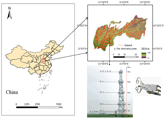
Figure 1.
The geographical position of study area.
The flux observation site is situated at the Xinxiang Comprehensive Test Base of the Chinese Academy of Agricultural Sciences, Qiliying Town, Xinxiang County, Henan Province (35°9’ 42” N, 113°47’ 42” E). It is equipped with a complete set of eddy covariance observation and meteorological gradient systems for real-time monitoring of water vapor fluxes and meteorological factors in agricultural fields.
2.2. Data
2.2.1. Remote Sensing Data
In this study, we selected 15 image data during the winter wheat growth period from 2019 to 2022 with less than 10% cloud conditions. As shown in Table 1, the data were obtained from Landsat-8 and Landsat-9 secondary products (downloaded address: https://earthexplorer.usgs.gov/, accessed on 30 September 2023). Landsat-9 launched on 27 September 2021 from Vandenberg Air Force Base, California, onboard a United Launch Alliance Atlas V 401 rocket. Landsat-9 carried the Operational Land Imager 2 (OLI–2) and the Thermal Infrared Sensor2 (TIRS–2). The satellite’s band resolution is consistent with that of Landsat-8, with a spatial resolution of up to 30 m in the multispectral band and 100 m in the thermal infrared band. However, its operating cycle is offset from Landsat-8 by 8 days, making it a useful complement to Landsat-8 and addressing the issue of data scarcity. The secondary products have undergone radiometric and atmospheric correction and only require mosaicking and cropping to extract the surface parameters of the study area [26].

Table 1.
Information of remote sensing data used in the study.
2.2.2. Digital Elevation Model
The ASTER GDEM model (download address: https://glovis.usgs.gov/, accessed on 30 September 2023) was used in the study with a spatial resolution of 30 m. The image was cropped to obtain a topographic elevation map of the study area.
2.2.3. Meteorological Data
The study utilized meteorological data obtained from GLDAS (download address: https://ldas.gsfc.nasa.gov/data, accessed on 30 September 2023). The data had a spatial resolution of 0.25° × 0.25° and a temporal resolution of 3 h. The meteorological elements extracted and resampled in ArcGIS included temperature, wind speed, barometric pressure, and relative humidity, which were used as input parameters for the SEBS model.
2.2.4. Validation Data
The measurements from eleven eddy covariance (EC) sites were used in the study. These data were provided by the flux observation site in Xinxiang Comprehensive Test Base of Chinese Academy of Agricultural Sciences. An eddy covariance observation system (acronym: EC system) and a meteorological gradient system were equipped. The EC system, with a height of 5 m, consisted of a three-dimensional ultrasonic anemometer (CSAT-3, Campbell Scientific Ine, Logan, UT, USA) and a closed-circuit gas analyzer (EC155, Campbell Scientific Ine, Logan, UT, USA). The three-dimensional wind speed, the virtual temperature, and the change of the water vapor concentration of the farmland were measured. The data were collected at a frequency of 10 Hz and an average period of 30 days. The meteorological gradient system consisted of air temperature sensors, wind speed sensors, rainfall sensors, and a CNR4 Net Radiometer (CNR4) at each level; it can be used to monitor the changes in meteorological elements at different heights.
2.3. Methodology
2.3.1. SEBS Model
The SEBS model is based on the theory of surface energy balance, and the model assumes that the underlying surface is homogeneous and widely covered by vegetation. The various meteorological parameters are used to calculate each part of the flux components, and the regional surface energy balance equation is formed [27]:
where is the net radiation flux, W/m2; is the sensible heat flux, W/m2; is the soil heat flux, W/m2; and represents the latent heat flux, W/m2.
Net radiation flux is the difference between the total radiation from the surface up and down. The calculation formula is as follows:
where is the surface albedo; is the downward solar radiation, W/m2; is the downward longwave radiation, W/m2; is the atmospheric emissivity; is the surface specific emissivity; is the Boltzmann constant, which is often taken to be 5.67 × 10⁻⁸ W∙m2∙k−4; is the surface temperature, K.
Soil heat flux is the main parameter of surface energy balance theory and is defined as the heat exchange of soil per unit area per unit time. The empirical statistical formula is as follows:
where is the coefficient of the size of the proportion of vegetation cover; is the vegetation cover rate; is the ratio coefficient of bare soil coverage. The ratio of soil heat flux to surface net radiation was assumed to be 0.05 and 0.315 for bare soil during model calculation.
Sensible heat flux is the heat exchange between atmospheric turbulence and underlying surface caused by temperature change. In order to derive sensible heat flux, the SEBS model distinguishes the atmospheric boundary layer ABL, planetary boundary layer PBL, and atmospheric surface layer ASL based on the boundary layer theory. The calculation formula is as follows:
where is the air density, g/m3; is the specific heat capacity of air, J/(kg∙k); is the potential virtual temperature near the surface, K; and is the gravitational acceleration, m/s2.
In the SEBS model, sensible heat flux and latent heat flux under dry and wet limits are usually considered, and the relative evaporation ratio can be expressed as
where is the relative evaporation ratio, it is a dimensionless constant, and the subscripts represent the dry limit and wet limit, respectively.
After calculating the relative evaporation ratio, the instantaneous ET is calculated according to the following formula:
where is the instantaneous ET, mm.
After calculating the instantaneous ET, the ET ratio is calculated according to the concept of relative ET ratio, and then the instantaneous ET is extended to the daily ET scale with the following formula:
where is the extended daily scale ET, mm; is the average daily ET ratio; is the average daily net radiation, W/m2; is the average daily soil heat flux, W/m2; is the latent heat of vaporization of water, J/kg; is the density of water, 103 kg∙m−3.
2.3.2. Data Mining Sharpener Model
The Data Mining Sharpener (DMS) model used in this paper is based on the machine learning method introduced by Gao in 2012 [17]. As a machine learning method, DMS uses regression decisions to establish the relationship between surface temperature (LST) and reflectance (R) at low resolution. The relationship between LST and R may vary depending on the scenario due to multiple factors. To address this, the DMS utilized a global regression model to select samples from the entire scenario. Additionally, the DMS implemented global and overlapping moving window methods on each scenario and combined the results based on the residuals between the regression outputs and the low-resolution training data. After the sharpening process, we analyzed the regression output and low-resolution data for residuals and bias correction. This ensures consistency between the high-resolution image elements and their corresponding low-resolution counterparts.
2.3.3. Statistical Metrics
This study used three indicators to validate the model inversion results, and the formulas are as follows:
is the ratio of the variance of the described variable, which measures how well the simulated value fits the measured value.
is the root mean square error, which measures the deviation between the predicted value and the true value, and it is more sensitive to outliers in the data.
is the mean absolute error, which indicates the average of the absolute error between the predicted value and the observed value, and it can reflect the true error.
is the number of samples, is the measured value, and is the model inversion value.
3. Results
3.1. Soil Information Extraction in the Study Area
Given the complexity of land surface information in the study area and the serious fragmentation of the area used for winter wheat crop cultivation, Landsat-8 imagery data on 30 December 2019 was selected; the maximum likelihood supervised classification method was adopted to extract the land use information of the area, and the accuracy of the classification results was evaluated to better explain the spatial and temporal distribution characteristics of winter wheat ET in the area.
The study area was classified into five land types using the maximum likelihood method, namely, building land, woodland, water, wheat, and other arable land, as shown in Figure 2. The remote sensing interpretation accuracy assessment revealed an overall classification accuracy of 96.4% and a kappa coefficient of 0.935.
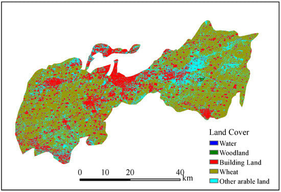
Figure 2.
Land use type map of the research area.
3.2. Evaluation of DMS
To verify the sharpened accuracy of the DMS model, the pixel values at the same latitude and longitude as the four-component radiometer erected on the flux tower were selected for comparison. Table 2 shows that the R2 was 0.961, which was between the LST at 100 m spatial resolution and the measured surface temperature by the CNR4, the RMSE was 0.968 °C, and the MAE was 2.236 °C. The R2 was 0.975, which was between the LST at 30 m spatial resolution and the measured surface temperature by the CNR4, the RMSE was 0.811 °C, and the MAE was 1.948 °C. The difference in surface temperature before and after sharpening was maintained between 1~2 °C. The correlation coefficients of the two thermal infrared images with different spatial resolutions were consistently above 0.9 [28]. Compared to the 100 m spatial resolution, the LST at 30 m spatial resolution showed improved accuracy. Additionally, the two spatial distributions appeared similar visually, and the 30 m spatial resolution surface temperature image provided better detail. The surface temperature image with a 100 m spatial resolution can represent the subsurface environment, which may include factories, roads, fields, and other features. In this case, the pixel value reflects the weighted average of the surface temperature of the complex environment. This is different from the measurement range of the quadruple-component radiometer. When the spatial resolution was improved to 30 m, the pixel value from the quadruple-component radiometer corresponded to only a small piece of agricultural land at the same latitude and longitude. This adjustment made the pixel value more accurate. Figure 3 showed that sharpening the resolution of independent pixels from 100 m to 30 m improved the texture of the image, made the boundary lines more distinct, and resulted in smoother surface temperature changes.
Table 2.
Comparison of ground surface temperature sharpened results.
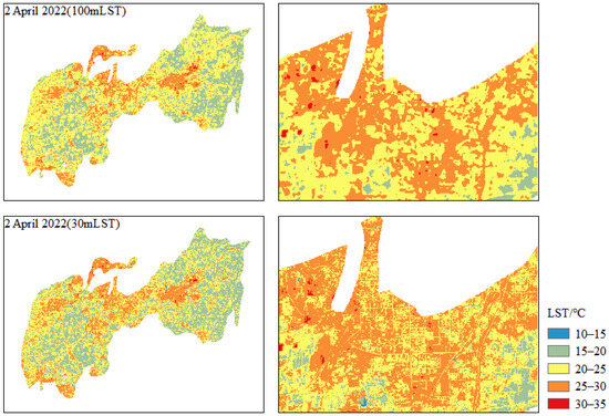
Figure 3.
Comparison chart of surface temperature before and after sharpening.
3.3. Evaluation of Sharpened ET
To verify the inversion accuracy of the SEBS model, the pixel values at the same latitude and longitude as the closed-circuit EC system were selected. The inversion results are shown in Table 3; the R2 between the 100 m spatial resolution of ET and the measured value by EC system reached 0.814, the RMSE was 0.516 mm, and the MAE was 0.245 mm. The R2 between the 30 m spatial resolution of ET and the measured value by EC system reached 0.802, the RMSE was 0.534 mm, and the MAE was 0.253 mm. Results showed that the accuracy of the ET inversion after sharpening was significantly improved compared with the previous one.
Table 3.
Comparison of daily ET results.
The People’s Victory Irrigation District spans the Yellow River and Haihe River basins. The water source of the irrigation district is mainly diverted from the Yellow River. A rotation system of winter wheat and summer corn is implemented throughout the year [29]. Figure 4 and Figure 5 illustrate the daily ET of winter wheat in the People’s Victory Irrigation District. The trend of ET gradually increases from east to west and from north to south, which is consistent with the layout of the farmland water conservancy system in this irrigation district. The southwest area of the People’s Victory Irrigation District has more trunk canals, complex canal system distribution, and abundant water resources. The daily evapotranspiration in the southwest area was significantly higher than that in the northeast area. Upon examining the land use type map of the irrigation area, it became apparent that the ET of water was higher than that of woodland, wheat, and other arable land. Although water areas and forest lands have the ability to contain water, their distribution is limited in the People’s Victory Irrigation area. Therefore, the ET in this irrigation area is primarily supplied by the winter wheat growing area. During the period of rapid winter wheat growth, the low NDVI of construction land may result in significant loss in ET estimation. This is particularly evident in the ET interpolation map with 30 m spatial resolution.
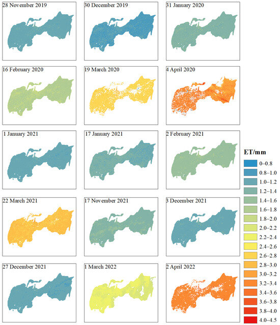
Figure 4.
Spatial and temporal distribution of daily ET.
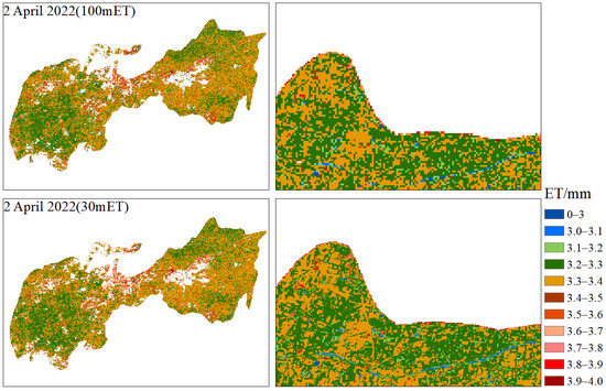
Figure 5.
Comparison of daily ET before and after downscaling.
Combined with the horizontal comparison of ET data over the years, it can be seen that the daily ET of winter wheat in the People’s Victory Drainage Irrigation District during different reproductive periods showed systematic changes. During the early growth stage, spanning from November to January, the ET of wheat exhibited a decreasing trend. This was due to the weak average daily temperature and net solar radiation, which resulted in relatively slow growth of the wheat. In February of the following year, as the temperature increased, the leaf area index of winter wheat and the vegetation coverage rate of the field gradually increased, leading to a change in the ET of winter wheat. After reaching the jointing and heading stages, the increase in air temperature and net solar radiation led to a further increase in transpiration and interplant evaporation of winter wheat. As a result, the daily water demand sharply increased, and the field evapotranspiration continued to rise. The growth of winter wheat was the most vigorous during the filling stage, with the largest leaf area index observed. The daily ET also reached its maximum value during the entire growth period. Following the filling stage, the winter wheat matured into grains gradually. The leaves began to fall off, and the ET started to decline again until the harvest was completed.
3.4. Analysis of ET Influence Factors
The SEBS model takes into account both surface and meteorological parameters. In this study, we analyzed the correlation between ET and meteorological data during the winter wheat growth period in 2019. The influencing factors considered were air temperature (Ta), relative humidity (RH), mean water vapor pressure (E), wind speed (WS), net solar radiation (Rn), soil temperature (Soil-T), soil moisture (Soil-VWC), and surface temperature (LST). We used SPSS for path analysis, and the specific results are shown in Table 4.
Table 4.
Path analysis table of field ET influence factors.
Field ET is the fundamental variable for turbulent exchange between crops, surface soils, and the atmosphere. The influencing factors are complex and have different proportions at different scales. Additionally, there are interactions between these factors. Table 4 shows the degree of influence of each factor on ET, with net solar radiation having the greatest influence, followed by surface temperature, air temperature, relative humidity, soil moisture, average water vapor pressure, and wind speed. The net solar radiation and temperature exhibited a highly significant positive correlation with ET, while humidity showed a negative correlation. Throughout the growth period, the net solar radiation served as the primary source of energy for the turbulent exchange between crops and soil, making it the most influential factor in ET changes. Temperature difference was the main gradient force between vegetation transpiration and soil evaporation. As the temperature increases, the capacity for both vegetation transpiration and soil evaporation also increases. While wind speed can enhance turbulence exchange speed between the atmosphere, its impact on water surface ET is more significant than on farmland ET. Relative humidity and soil moisture are both significantly and negatively correlated with ET. In agricultural production, high humidity can reduce the saturated water vapor pressure difference and weaken the driving force for evapotranspiration. This can affect plant transpiration and cause a decline in evapotranspiration in farmland. The net solar radiation Rn has the greatest effect on ET, with a direct flux coefficient of 0.992 and an indirect flux coefficient of 1.926. The second most influential factor on ET is air temperature, with its direct effect being greater than its indirect effect. Changes in air temperature can cause fluctuations in mean water vapor pressure and soil temperature, which in turn affect ET.
4. Discussion
The Landsat series of satellites have provided a long series of thermal infrared (TIR) observations, which are a valuable data source for acquiring surface temperature [30]. The Landsat-9 and Landsat-8 products used in the study showed good consistency, but some areas were seriously affected by cloud shadows. During the cropping process, the phenomenon of blank banding occurs in the non-study area portion of the image. Meng et al, discovered that the occurrence of blank banding in Landsat-9 LST products was due to its surface temperature algorithm. This issue can be resolved by using the gap elimination method or alternative surface temperature algorithms [26].
Cheng et al. conducted downscaling research using thermal infrared data from kilometer-scale satellites such as MODIS or Sentinel-3. The data were compared with the thermal infrared band of Landsat, which has a 100 m scale, to achieve a more pronounced downscaling effect [31]. However, downsizing the thermal infrared data from kilometer-scale to 100 m made it difficult to ensure the accuracy and completeness of the results [32], and there was a high likelihood that data were lost during the temperature reconstruction process [33]. In this study, Landsat thermal infrared data with a resolution of 100 m were sharpened to 30 m, which is consistent with Gao’s original idea. The distribution of land surface temperature at a spatial resolution of 100 m after sharpening was found to be similar to that at 30 m resolution. The sharpening process did not significantly alter the temperature distribution. The surface temperature at 30 m resolution was found to be more accurate when compared to the measured data of the CNR4. As a result, the evaluation index also improved.
SEBS is a single-source surface energy balance model, which estimates atmospheric turbulent fluxes and surface evaporative fraction from remote sensing data. It has been applied and validated in many places, but there are even fewer studies on crop water demand for winter wheat growing areas in Henan Province with long time series. In the study, the evapotranspiration problem of winter wheat in the People’s Victory Irrigation District of Henan Province was estimated by using Landsat data and meteorological data for 3 years, and the inversion results were compared with the measured data. After scaling down, the correlation coefficient R2 between the inversion value of the SEBS model and the measured vorticity value reached 0.814, it had a high inversion accuracy, and the results were similar to the conclusion drawn by Zhang and Jiang. Based on the SEBS model, Zhang conducted experiments on the inversion of ET under two scenarios of using MODIS remote sensing data alone and MODIS integrated with VIIRS remote sensing data, respectively. After verifying the accuracy of the evapotranspiration results, it was found that the accuracy of evapotranspiration was improved by the integration of VIIRS remote sensing data [34]. Estimation of evapotranspiration of winter wheat at different fertility stages based on Landsat-8 remote sensing data was carried out in Liangyuan District, Shangqiu City, Henan Province, China, by Jiang [35] Secondly, the temporal and spatial distribution of daily evapotranspiration after downscaling was essentially the same as before downscaling. The inversion accuracy slightly improved compared to before downscaling, which increased the reliability of ET after downscaling. From a visual perspective, Figure 5 illustrates that the daily ET distribution map with 30 m spatial resolution and that with 100 m resolution were significantly different in detail, particularly near the boundary line. The effect of downscaling was evident, and in some areas with complex underlying surface conditions, such as the intersection of cultivated land and construction land, the daily ET map after downscaling did not show a clear mosaic phenomenon, and the changes in ET were smoother.
From the research process described above, some deficiencies in the study were identified. Firstly, the use of DMS to determine the limitations of surface temperature sharpening was found to be inadequate. There was a correlation between LST and R in different scenarios [36]. Guzinski showed that thermal infrared images and reflectance can capture this information in the case of crop water stress, which has led to the two becoming complementary [18]. The surface conditions of the observation area selected for the study were similar to those of the crop. Specifically, the selected observation area had good water holding capacity and did not exhibit any signs of drought. Therefore, it is necessary to discuss in depth whether DMS is suitable for early monitoring of water stress or precision irrigation. In this study, a significant difference was observed between the measured value and the inversion value. For instance, on 19 March 2020, the actual ET value was 4.732 mm, which differed greatly from the inversion value. This difference could be attributed to the jointing period of winter wheat and the manmade irrigation treatment in the field. When the field experiences rainfall or manmade full irrigation, the ET in the field will increase within two or three days, which can distort the measured data. The input parameters for the SEBS model, based on the energy balance formula, include the normalized vegetation index, surface temperature, and surface albedo. Excluding soil moisture information could hinder obtaining these parameters in a timely manner, which may impede the energy balance model’s ability to estimate surface ET in real time [37].
Until a new generation of thermal satellites is launched, DMS will be a useful solution for overcoming the lack of thermal data, which has led to the lack of real-time performance of the energy balance model in estimating surface ET [38]. This method can even be combined with UAV to monitor crop water requirements at smaller scales if higher spatial resolution is required. On the other hand, we chose to use simultaneous sensors [39]. Simultaneous sensor acquisitions from the same platform represent the best-case scenario for estimating evapotranspiration (ET) due to inherent advantages over multisource sensors. This approach ensures input consistency between land surface temperature (LST) and vegetation indices for ET models. When combining multiple sensors for an experiment, it is important to maximize scene coverage, avoid image misalignments due to sensor registration differences, and enable improved cloud detection [40].
5. Conclusions
The study utilized the DMS surface temperature sharpened model, the SEBS model, and multiyear Landsat image data to estimate the daily ET during the growth period of winter wheat in the People’s Victory Irrigation District. The results indicate that the accuracy of surface temperature and daily ET at 30 m spatial resolution after downscaling improved to varying degrees. The study adhered to the initial concept of the experimental results. Compared to the longitudinal interpolated map with a 100 m resolution, the downscaling process provided more specific details on the distribution of surface temperature and daily ET, making complex regional differences more apparent. This demonstrates the feasibility of using DMS to downscale land surface temperature from the Landsat satellite and verifies the applicability of the SEBS model in Henan Province. By analyzing the spatiotemporal distribution of ET during different growth stages of winter wheat, it was found that ET in the southwest was significantly higher than that in the northeast. Throughout the growth period, the daily average ET of winter wheat exhibited a pattern of decreasing, then increasing, and then decreasing again. The analysis of factors influencing ET reveals that net solar radiation and temperature have a highly significant positive correlation with ET. Wind speed has a weaker correlation with ET, while relative humidity and soil moisture are both significantly negatively correlated with ET. The direct and indirect path coefficients indicate that net solar radiation has the greatest influence on ET and plays a promoting role.
Author Contributions
Conceptualization, J.Z.; methodology, J.Z.; formal analysis, J.Z. and S.L.; data curation, J.Z.; writing—reviewing and editing, Z.C. and J.W.; funding acquisition, Z.C.; project administration, J.W. All authors have read and agreed to the published version of the manuscript.
Funding
This research was funded by the Key Program of Science and Technology in Henan Province (No. 21100110700), National Key R&D Program of China (No. 2022YFD1900502), Innovation Mechanism of Modern Agricultural Research Institutes (No. Y2022ZK30).
Data Availability Statement
Data are contained within the article.
Acknowledgments
We would like to thank the anonymous reviewers for their long-term guidance and constructive comments.
Conflicts of Interest
The authors declare no conflict of interest.
Correction Statement
This article has been republished with a minor correction to the existing affiliation information. This change does not affect the scientific content of the article.
References
- Katul, G.G.; Oren, R.; Manzoni, S.; Higgins, C.; Parlange, M.B. Evapotranspiration: A process driving mass transport and energy exchange in the soil-plant-atmosphere-climate system. Rev. Geophys. 2012, 50, 3. [Google Scholar] [CrossRef]
- Wang, S.; Wang, C.; Zhang, C.; Xue, J.; Wang, P.; Wang, X.; Wang, W.; Zhang, X.; Li, W.; Huang, G.; et al. A classification-based spatiotemporal adaptive fusion model for the evaluation of remotely sensed evapotranspiration in heterogeneous irrigated agricultural area. Remote Sens. Environ. 2022, 273, 112962. [Google Scholar] [CrossRef]
- Weiss, M.; Jacob, F.; Duveiller, G. Remote sensing for agricultural applications: A meta-review. Remote Sens. Environ. 2020, 236, 111402. [Google Scholar] [CrossRef]
- Song, L.; Liu, S.; Xu, T.; Xu, Z.; Ma, Y. Soil evaporation and vegetation transpiration: Remotely sensed estimation and validation. J. Remote Sens. 2017, 21, 966–981. [Google Scholar] [CrossRef]
- Zhaoliang, L.; Sibo, D.; Bohui, T.; Hua, W.U.; Huazhong, R.E.N.; Guangjian, Y.A.N.; Ronglin, T.; Pei, L. Review of methods for land surface temperature derived from thermal infrared remotely sensed data. J. Remote Sens. 2016, 20, 899–920. [Google Scholar] [CrossRef]
- Chen, Z.; Ren, J.; Tang, H.; Shi, Y.; Leng, P.; Liu, J.; Wang, L.; Wu, W.; Yao, Y.; Hasiyuya, T. Progress and perspectives on agricultural remote sensing research and applications in China. J. Remote Sens. 2016, 20, 748–767. [Google Scholar]
- Liang, S.; Bai, R.; Chen, X.; Cheng, J.; Fan, W.; He, T.; Jia, K.; Jiang, B.; Jiang, L.; Jiao, Z.; et al. Review of China’s land surface quantitative remote sensing development in 2019. J. Remote Sens. 2020, 24, 618–671. [Google Scholar]
- Li, S.; Wang, J.; Li, D.; Ran, Z.; Yang, B. Evaluation of Landsat 8-like Land Surface Temperature by Fusing Landsat 8 and MODIS Land Surface Temperature Product. Processes 2021, 9, 2262. [Google Scholar] [CrossRef]
- Anderson, M.; Gao, F.; Knipper, K.; Hain, C.; Dulaney, W.; Baldocchi, D.; Eichelmann, E.; Hemes, K.; Yang, Y.; Medellin-Azuara, J.; et al. Field-Scale Assessment of Land and Water Use Change over the California Delta Using Remote Sensing. Remote Sens. 2018, 10, 889. [Google Scholar] [CrossRef]
- Firozjaei, M.K.; Kiavarz, M.; Alavipanah, S.K. Satellite-derived land surface temperature spatial sharpening: A comprehensive review on current status and perspectives. Eur. J. Remote Sens. 2022, 55, 644–664. [Google Scholar] [CrossRef]
- Mokhtari, A.; Noory, H.; Pourshakouri, F.; Haghighatmehr, P.; Afrasiabian, Y.; Razavi, M.; Fereydooni, F.; Sadeghi Naeni, A. Calculating potential evapotranspiration and single crop coefficient based on energy balance equation using Landsat 8 and Sentinel-2. ISPRS J. Photogramm. Remote Sens. 2019, 154, 231–245. [Google Scholar] [CrossRef]
- Ha, W.; Gowda, P.H.; Howell, T.A. Downscaling of Land Surface Temperature Maps in the Texas High Plains with the TsHARP Method. GISci. Remote Sens. 2011, 48, 583–599. [Google Scholar] [CrossRef]
- Mukherjee, S.; Joshi, P.K.; Garg, R.D. Evaluation of LST downscaling algorithms on seasonal thermal data in humid subtropical regions of India. Int. J. Remote Sens. 2015, 36, 2503–2523. [Google Scholar] [CrossRef]
- Sattari, F.; Hashim, M.; Sookhak, M.; Banihashemi, S.; Pour, A.B. Assessment of the TsHARP method for spatial downscaling of land surface temperature over urban regions. Urban Clim. 2022, 45, 101265. [Google Scholar] [CrossRef]
- Huang, S.; Zhang, X.; Wang, C.; Chen, N. Two-step fusion method for generating 1 km seamless multi-layer soil moisture with high accuracy in the Qinghai-Tibet plateau. ISPRS J. Photogramm. Remote Sens. 2023, 197, 346–363. [Google Scholar] [CrossRef]
- Bai, Y.; Wong, M.; Shi, W.Z.; Wu, L.X.; Qin, K. Advancing of Land Surface Temperature Retrieval Using Extreme Learning Machine and Spatio-Temporal Adaptive Data Fusion Algorithm. Remote Sens. 2015, 7, 4424–4441. [Google Scholar] [CrossRef]
- Gao, F.; Kustas, W.; Anderson, M. A Data Mining Approach for Sharpening Thermal Satellite Imagery over Land. Remote Sens. 2012, 4, 3287–3319. [Google Scholar] [CrossRef]
- Guzinski, R.; Nieto, H. Evaluating the feasibility of using Sentinel-2 and Sentinel-3 satellites for high-resolution evapotranspiration estimations. Remote Sens. Environ. 2019, 221, 157–172. [Google Scholar] [CrossRef]
- Fisher, J.B.; Melton, F.; Middleton, E.; Hain, C.; Anderson, M.; Allen, R.; McCabe, M.F.; Hook, S.; Baldocchi, D.; Townsend, P.A.; et al. The future of evapotranspiration: Global requirements for ecosystem functioning, carbon and climate feedbacks, agricultural management, and water resources. Water Resour. Res. 2017, 53, 2618–2626. [Google Scholar] [CrossRef]
- Xu, S.; Cheng, J. A new land surface temperature fusion strategy based on cumulative distribution function matching and multiresolution Kalman filtering. Remote Sens. Environ. 2021, 254, 112256. [Google Scholar] [CrossRef]
- Liu, K.; Su, H.; Li, X.; Chen, S. Development of a 250-m Downscaled Land Surface Temperature Data Set and its Application to Improving Remotely Sensed Evapotranspiration Over Large Landscapes in Northern China. IEEE Trans. Geosci. Remote Sens. 2022, 60, 5000112. [Google Scholar] [CrossRef]
- Liu, J.; Si, Z.; Li, S.; Kader Mounkaila Hamani, A.; Zhang, Y.; Wu, L.; Gao, Y.; Duan, A. Variations in water sources used by winter wheat across distinct rainfall years in the North China Plain. J. Hydrol. 2023, 618, 129186. [Google Scholar] [CrossRef]
- Liu, J.; Si, Z.; Wu, L.; Chen, J.; Gao, Y.; Duan, A. Using stable isotopes to quantify root water uptake under a new planting pattern of high-low seed beds cultivation in winter wheat. Soil. Tillage Res. 2021, 205, 104816. [Google Scholar] [CrossRef]
- Liu, J.; Si, Z.; Wu, L.; Shen, X.; Gao, Y.; Duan, A. High-low seedbed cultivation drives the efficient utilization of key production resources and the improvement of wheat productivity in the North China Plain. Agr. Water. Manag. 2023, 285, 108357. [Google Scholar] [CrossRef]
- Chang, D.; Huang, Z.; Qi, X.; Han, Y.; Liang, Z. Analysis on spatio-temporal variability and influencing factors of net irrigation requirement in People’s Victory Canal Irrigation Area. Chin. Soc. Agric. Eng. 2017, 33, 118–125. [Google Scholar]
- Meng, X.; Cheng, J.; Guo, H.; Guo, Y.; Yao, B. Accuracy Evaluation of the Landsat 9 Land Surface Temperature Product. IEEE J. Sel. Top. Appl. Earth Obs. Remote Sens. 2022, 15, 8694–8703. [Google Scholar] [CrossRef]
- Su, Z. The Surface Energy Balance System (SEBS) for estimation of turbulent heat fluxes. Hydrol. Earth Syst. Sci. 2002, 6, 85–100. [Google Scholar] [CrossRef]
- Zhao, G.; Zhang, Y.; Tan, J.; Li, C.; Ren, Y. A Data Fusion Modeling Framework for Retrieval of Land Surface Temperature from Landsat-8 and MODIS Data. Sensors 2020, 20, 4337. [Google Scholar] [CrossRef]
- Zhang, C.; Long, D.; Zhang, Y.; Anderson, M.C.; Kustas, W.P.; Yang, Y. A decadal (2008–2017) daily evapotranspiration data set of 1 km spatial resolution and spatial completeness across the North China Plain using TSEB and data fusion. Remote Sens. Environ. 2021, 262, 112519. [Google Scholar] [CrossRef]
- Duan, S.B.; Li, Z.L.; Zhao, W.; Wu, P.; Huang, C.; Han, X.J.; Gao, M.; Leng, P.; Shang, G. Validation of Landsat land surface temperature product in the conterminous United States using in situ measurements from SURFRAD, ARM, and NDBC sites. Int. J. Digit. Earth 2020, 14, 640–660. [Google Scholar] [CrossRef]
- Cheng, L.; Liu, S.; Mo, X.; Hu, S.; Zhou, H.; Xie, C.; Nielsen, S.; Grosen, H.; Bauer-Gottwein, P. Assessing the Potential of 10-m Resolution TVDI Based on Downscaled LST to Monitor Soil Moisture in Tang River Basin, China. Remote Sens. 2023, 15, 744. [Google Scholar] [CrossRef]
- Bellvert, J.; Jofre-Cekalovic, C.; Pelecha, A.; Mata, M.; Nieto, H. Feasibility of Using the Two-Source Energy Balance Model (TSEB) with Sentinel-2 and Sentinel-3 Images to Analyze the Spatio-Temporal Variability of Vine Water Status in a Vineyard. Remote Sens. 2020, 12, 14. [Google Scholar] [CrossRef]
- Aguirre-García, S.D.; Aranda-Barranco, S.; Nieto, H.; Serrano-Ortiz, P.; Sánchez-Cañete, E.P.; Guerrero-Rascado, J.L. Modelling actual evapotranspiration using a two source energy balance model with Sentinel imagery in herbaceous-free and herbaceous-cover Mediterranean olive orchards. Agr. Forest. Meteorol. 2021, 311, 108692. [Google Scholar] [CrossRef]
- Zhang, Y. Estimation of ET in Wheat Area of Henan Province Based on SEBS Model. Ph.D. Thesis, Zhengzhou University, Zhengzhou, China, 2019. [Google Scholar]
- Jiang, B.; Meng, D.; Guo, X.; Zhu, L. Spatial and temporal distribution of surface ET in winter wheat planting area based on Landsat-8 remote sensing data. Irrig. Drain. 2022, 41, 140–146. [Google Scholar]
- Geli, H.M.E.; González-Piqueras, J.; Neale, C.M.U.; Balbontín, C.; Campos, I.; Calera, A. Effects of Surface Heterogeneity Due to Drip Irrigation on Scintillometer Estimates of Sensible, Latent Heat Fluxes and Evapotranspiration over Vineyards. Water 2019, 12, 81. [Google Scholar] [CrossRef]
- Guzinski, R.; Nieto, H.; Sandholt, I.; Karamitilios, G. Modelling High-Resolution Actual Evapotranspiration through Sentinel-2 and Sentinel-3 Data Fusion. Remote Sens. 2020, 12, 1433. [Google Scholar] [CrossRef]
- Xue, J.; Anderson, M.C.; Gao, F.; Hain, C.; Yang, Y.; Knipper, K.R.; Kustas, W.P.; Yang, Y. Mapping Daily Evapotranspiration at Field Scale Using the Harmonized Landsat and Sentinel-2 Dataset, with Sharpened VIIRS as a Sentinel-2 Thermal Proxy. Remote Sens. 2021, 13, 3420. [Google Scholar] [CrossRef]
- Yang, Y.; Anderson, M.; Gao, F.; Hain, C.; Noormets, A.; Sun, G.; Wynne, R.; Thomas, V.; Sun, L. Investigating impacts of drought and disturbance on evapotranspiration over a forested landscape in North Carolina, USA using high spatiotemporal resolution remotely sensed data. Remote Sens. Environ. 2020, 238, 111018. [Google Scholar] [CrossRef]
- Semmens, K.A.; Anderson, M.C.; Kustas, W.P.; Gao, F.; Alfieri, J.G.; McKee, L.; Prueger, J.H.; Hain, C.R.; Cammalleri, C.; Yang, Y.; et al. Monitoring daily evapotranspiration over two California vineyards using Landsat 8 in a multi-sensor data fusion approach. Remote Sens. Environ. 2016, 185, 155–170. [Google Scholar] [CrossRef]
Disclaimer/Publisher’s Note: The statements, opinions and data contained in all publications are solely those of the individual author(s) and contributor(s) and not of MDPI and/or the editor(s). MDPI and/or the editor(s) disclaim responsibility for any injury to people or property resulting from any ideas, methods, instructions or products referred to in the content. |
© 2023 by the authors. Licensee MDPI, Basel, Switzerland. This article is an open access article distributed under the terms and conditions of the Creative Commons Attribution (CC BY) license (https://creativecommons.org/licenses/by/4.0/).