An Approach to Chance Constrained Problems Based on Huge Data Sets Using Weighted Stratified Sampling and Adaptive Differential Evolution ^†

Abstract

In this paper, a new approach to solve Chance Constrained Problems (CCPs) using huge data sets is proposed. Specifically, instead of the conventional mathematical model, a huge data set is used to formulate CCP. This is because such a large data set is available nowadays due to advanced information technologies. Since the data set is too large to evaluate the probabilistic constraint of CCP, a new data reduction method called Weighted Stratified Sampling (WSS) is proposed to describe a relaxation problem of CCP. An adaptive Differential Evolution combined with a pruning technique is also proposed to solve the relaxation problem of CCP efficiently. The performance of WSS is compared with a well known method, Simple Random Sampling. Then, the proposed approach is applied to a real-world application, namely the flood control planning formulated as CCP.

1. Introduction

In real-world applications, a wide range of uncertainties have to be taken into account. Therefore, optimization problems under uncertainties have been studied for many years. Generally speaking, there are two types of formulations for handling uncertainties in optimization problems. The first one is the deterministic optimization problem [1]. The second one is the stochastic optimization problem [2]. The robust optimization problem is a well-known deterministic formulation [1]. The robust optimization problem always considers the worst-case performance under uncertainties. Therefore, the overestimation of uncertainties may lead to a conservative decision in practice.

The Chance Constrained Problem (CCP), which is also referred to as the probabilistic constrained problem [3], is one of the possible formulations of the stochastic optimization problem. CCP is a risk-averse formulation of problem under uncertainties. Specifically, CCP ensures that the probability of meeting all constraints is above a certain level. Since the balance between optimality and reliability can be designated by CCP, many real-world applications have been formulated as CCPs [3,4,5].

CCP has been studied in the field of stochastic programming for many years [2]. In stochastic programming, the optimization methods of the nonlinear programming [6] have been used to solve CCP. Recently, Evolutionary Algorithms (EAs) have also been reported for solving CCPs [7,8,9]. However, in the conventional formulation of CCP, a well known probability distribution such as the normal distribution is used widely as a mathematical model of unknown uncertainties. Then, the pseudo data generated randomly by using the Monte Carlo method based on the mathematical model are used to represent uncertainties [10]. In some cases, the mathematical model is used to derive a deterministic formulation of CCP [2,11]. Otherwise, very few data, or scenarios, observed actually are used to represent uncertainties. As a drawback of the conventional formulation of CCP, the estimation error of uncertainties is unavoidable in the evaluation of solutions. In other words, if CCP is defined incompletely, the solution is also defective. Then, we cannot enjoy the benefit of CCP.

In recent years, due to advanced information technologies such as Wireless Sensor Networks (WSN) and Internet of Things (IoT) [12], huge data sets called “big data” have been easily obtained in various fields including culture, science, and industry [13]. In many real-world applications, the variance of observed data is caused by some uncertainties. These applications are probably formulated as CCP more accurately by using a large data set instead of the mathematical model.

In this paper, CCP was formulated by using a large data set called a full data set. However, we assumed that the full data set is too large to solve CCP practically. Therefore, in order to evaluate solutions of CCP, we had to reduce the size of the full data set. Clustering is a popular data reduction technique [14]. Clustering divides a data set into some subsets in order to meet two requirements: “Internal cohesion” and “External isolation”. As a drawback of clustering, the result of clustering depends on the structure of data. Moreover, it is not good at dealing with a huge data set [15].

Sampling is another technique of data reduction. In particular, Simple Random Sampling (SRS) is widely used due to its easy execution and simplicity [16]. SRS selects a few samples randomly from a huge data set and discards most of data. As a drawback of SRS, the key information in many data is likely to be lost. Therefore, a new data reduction method called Weighted Stratified Sampling (WSS) has been proposed by authors to use the full data set completely for solving CCP [17].

By using the new data reduction method called WSS, the above CCP based on the full data set is converted into a relaxation problem of CCP. In order to solve the relaxation problem of CCP efficiently, a new optimization method based on Differential Evolution (DE) [18] is also contrived in this paper. In the new optimization method, a pruning technique is introduced into an adaptive DE [19] for reducing the number of candidate solutions to be examined on the process of the optimization.

The proposed approach is applied to a real-world application, namely the flood control planning formulated as CCP [5]. In addition to the conventional reservoir, the water-retaining capacity of the forest is considered in the flood control planning. Incidentally, various reservoir systems have been studied for protecting a downstream area of river from flood damage [20,21,22]. Even though historical data are used in these studies, many of them have been limited to dealing with problems of deterministic formulation. A stochastic formulation such as CCP is generally a more realistic representation of the flood control planning because stream flows have randomness and are stochastic in nature.

This paper is an extended version of the paper presented in ICIST2019 [17] and differs from the conference paper in the following three points: (1) The necessary sample size for SRS is derived theoretically. Then, it is shown that the theoretical sample size is too large in practice; (2) By using larger data sets, the performance of WSS is examined more intensively by comparison with SRS. Then, it is proven that WSS outperforms SRS in the accuracy of the estimated probability; (3) The ability of the pruning technique to reduce the run time of the adaptive DE is evaluated. Then, it is shown that the effect of the pruning technique increases proportionally to the sample size of WSS.

The remainder of this paper is organized as follows. Section 2 formulates CCP from a full data set. Section 3 explains two data reduction methods, namely the conventional SRS and the proposed WSS. By using a data reduction method, a relaxation problem of CCP is also derived. Section 4 proposes an adaptive DE combined with a pruning technique for solving the relaxation problem of CCP efficiently. Section 5 examines the performance of WSS intensively by comparison with SRS. Section 6 applies the proposed approach to a real-world application, namely the flood control planning formulated as CCP. Section 7 evaluates the ability of the pruning technique to reduce the run time of the adaptive DE on a personal computer. Finally, Section 8 concludes this paper and provides future work.

2. Problem Formulation

In this paper, uncertainties are represented by a vector of random variables $\mathit{\xi }\in \mathbf{\Omega }$ with a sample space $\mathbf{\Omega }\subseteq {\Re }^K$. The collection of vectors $\mathit{\xi }\in \mathbf{\Omega }\subseteq {\Re }^K$ is independent and identically distributed (i.i.d.). It is not necessarily that the collection of the elements ${\xi }_j\in \Re$ of each vector $\mathit{\xi }\in {\Re }^K$ is i.i.d. We suppose that both the sample space $\mathbf{\Omega }\subseteq {\Re }^K$ and the distribution of $\mathit{\xi }\in \mathbf{\Omega }$ are unknown. However, a full data set $\mathit{B}\subseteq \mathbf{\Omega }$ including a huge number of data ${\mathit{\xi }}^{\ell }\in \mathit{B}$ is available. Incidentally, the full data set can be regarded as a kind of “big data”. Symbols used in this paper are defined as follows:

• A vector of decision variables $\mathit{x}=(x_1,\cdots ,x_D)\in \mathit{X}\subseteq {\Re }^D$
• A vector of random variables $\mathit{\xi }=({\xi }_1,\cdots ,{\xi }_K)\in \mathbf{\Omega }\subseteq {\Re }^K$
• A huge number of data, or a full data set ${\mathit{\xi }}^{\ell }\in \mathit{B}\subseteq \mathbf{\Omega }$
• Measurable function for constraints $g_m:\mathit{X}\times \mathbf{\Omega }\to \Re$, $m=1,\cdots ,M$
• Objective function to be minimized $f:\mathit{X}\to \Re$
• Sufficiency level given by a probability $\alpha \in (0,1)$.

2.1. Chance Constrained Problem (CCP)

Let $Pr(\mathcal{A})$ be the probability that an event $\mathcal{A}$ occurs. The joint probability meeting all probabilistic constraints $g_m(\mathit{x},\mathit{\xi })\le 0$, $m=1,\cdots ,M$ for a solution $\mathit{x}\in \mathit{X}$ is described as

$$p(\mathit{x},\mathbf{\Omega })=Pr(\forall \mathit{\xi }\in \mathbf{\Omega }:g_m(\mathit{x},\mathit{\xi })\le 0,m=1,\cdots ,M).$$

(1)

By using the probability in (1), CCP is formulated as

$$\underset{\mathit{x}\in \mathit{X}}{min}f(\mathit{x})\mathrm{sub}.\mathrm{to}p(\mathit{x},\mathbf{\Omega })\ge \alpha$$

(2)

where a sufficiency level $\alpha \in (0,1)$ is given by an arbitrary probability.

In real-world applications, both the sample space $\mathbf{\Omega }\subseteq {\Re }^K$ and the distribution of $\mathit{\xi }\in \mathbf{\Omega }$ are usually unknown. Therefore, it is impossible to solve CCP in (2) directly.

2.2. Equivalence Problem of CCP

As stated above, due to advanced information technology, we can suppose that a huge data set $\mathit{B}=\{{\mathit{\xi }}^{\ell }\}\subseteq \mathbf{\Omega }$ is available for estimating the unknown probability $p(\mathit{x},\mathbf{\Omega })$ in (1) empirically.

First of all, the indicator function is defined as

$${\displaystyle \mathbb{𝟙}(g_m(\mathit{x},{\mathit{\xi }}^{\ell })\le 0)=\left\{\begin{array}{ccc}1\hfill & & \mathrm{if}{g}_m(\mathit{x},{\mathit{\xi }}^{\ell })\le 0\hfill \\ 0\hfill & & \mathrm{otherwise}.\hfill \end{array}\right.}$$

(3)

By using the indicator function in (3), the unknown probability $p(\mathit{x},\mathbf{\Omega })$ in (1) can be evaluated empirically from a huge number of data ${\mathit{\xi }}^{\ell }\in \mathit{B}$ for a solution $\mathit{x}\in \mathit{X}$ as

$${\displaystyle \widehat{p}(\mathit{x},\mathit{B})=\frac{1}{\left|\mathit{B}\right|}\sum _{{\mathit{\xi }}^{\ell }\in \mathit{B}}\left(\prod _{m=1}^M\mathbb{𝟙}(g_m(\mathit{x},{\mathit{\xi }}^{\ell })\le 0)\right)}$$

(4)

where $\left|\mathit{B}\right|$ denotes the size of the data set $\mathit{B}$, or the total number of data ${\mathit{\xi }}^{\ell }\in \mathit{B}$.

From the law of large numbers [23], we can expect that $p(\mathit{x},\mathbf{\Omega })\simeq \widehat{p}(\mathit{x},\mathit{B})$ holds. Therefore, by using the empirical probability in (4), CCP in (2) can be rewritten as

$$\underset{\mathit{x}\in \mathit{X}}{min}f(\mathit{x})\mathrm{sub}.\mathrm{to}\widehat{p}(\mathit{x},\mathit{B})\ge \alpha .$$

(5)

It is difficult to solve CCP in (5). In real-world applications, the function value $g_m(\mathit{x},{\mathit{\xi }}^{\ell })$ in (4) has to be evaluated for each of the data ${\mathit{\xi }}^{\ell }\in \mathit{B}$ through a time-consuming computer simulation. Thus, the full data set $\mathit{B}$ is too large to evaluate the empirical probability in (4). In order to solve CCP in (5) practically, we need to reduce the number of data ${\mathit{\xi }}^{\ell }\in \mathit{B}$ included in the full data set.

3. Data Reduction Methods

In order to reduce the number of data ${\mathit{\xi }}^{\ell }\in \mathit{B}$ included in the full data set $\mathit{B}\subseteq {\Re }^K$, we explain two data reduction methods. Firstly, Simple Random Sampling (SRS) is the most popular method [24]. SRS is widely used due to its easy execution and simplicity [25]. Secondly, Weighted Stratified Sampling (WSS) is a new data reduction method proposed by authors in ICIST 2019 [17].

3.1. Simple Random Sampling (SRS)

3.1.1. Procedure of SRS

Some samples ${\mathit{\xi }}^n\in \mathit{B}$, $n=1,\cdots ,N$ are selected randomly from the full data set for making a sample set $\mathbf{\Xi }=\{{\mathit{\xi }}^1,\cdots ,{\mathit{\xi }}^N\}\subseteq \mathit{B}$. The sample size N is far smaller than the data size $\left|\mathit{B}\right|$. By using samples ${\mathit{\xi }}^n\in \mathbf{\Xi }$, $n=1,\cdots ,N$ selected by SRS, an empirical probability is calculated as

$${\displaystyle \widehat{p}(\mathit{x},\mathbf{\Xi })=\frac{1}{N}\sum _{n=1}^N\left(\prod _{m=1}^M\mathbb{𝟙}(g_m(\mathit{x},{\mathit{\xi }}^n)\le 0)\right).}$$

(6)

The empirical probability $\widehat{p}(\mathit{x},\mathbf{\Xi })$ in (6) can be used to approximate $\widehat{p}(\mathit{x},\mathit{B})$ in (4).

3.1.2. Theoretical Sample Size

Supposing that $\widehat{p}(\mathit{x},\mathit{B})\simeq p(\mathit{x},\mathbf{\Omega })$ holds, we can estimate theoretically a necessary sample size for SRS. Let $\mathit{x}\in \mathit{X}$ be a solution of CCP in (5). By using random samples ${\mathit{\xi }}^n\in \mathbf{\Xi }\subseteq \mathit{B}$, $n=1,\cdots ,N$, the empirical probability $\widehat{p}(\mathit{x},\mathbf{\Xi })$ in (6) is evaluated from $y_n\in \{0,1\}$ defined as

$${\displaystyle y_n=\prod _{m=1}^M\mathbb{𝟙}(g_m(\mathit{x},{\mathit{\xi }}^n)\le 0).}$$

(7)

The values of $y_n\in \{0,1\}$ in (7), which depend on random samples ${\mathit{\xi }}^n\in \mathbf{\Xi }$, $n=1,\cdots ,N$, are regarded as random variables obeying a binomial distribution. From the central limit theorem, the binomial distribution can be approximated by a normal distribution [23]. Therefore, for any $ϵ\in (0,1)$ and $\delta \in (0,1)$, the confidence interval of the unknown probability $\widehat{p}(\mathit{x},\mathit{B})$ in (4) is described as

$${\displaystyle Pr\left(\left|\widehat{p}(\mathit{x},\mathit{B})-\widehat{p}(\mathit{x},\mathbf{\Xi })\right|\le \epsilon \right)\ge 1-\delta .}$$

(8)

Let $\Phi :\Re \to [0,1]$ be the Cumulative Distribution Function (CDF) of the standard normal distribution. From (8), the risk of failure $\delta \in (0,1)$ is derived as

$${\displaystyle \delta \ge 2\Phi \left(-\epsilon \sqrt{\frac{N}{\widehat{p}(\mathit{x},\mathit{B})(1-\widehat{p}(\mathit{x},\mathit{B}))}}\right).}$$

(9)

From (9), the margin of error $\epsilon \in (0,1)$ is also derived as

$${\displaystyle \epsilon \ge z_{\delta /2}\sqrt{\frac{\widehat{p}(\mathit{x},\mathit{B})(1-\widehat{p}(\mathit{x},\mathit{B}))}{N}}}$$

(10)

where $z_{\delta /2}\in [0.5,\infty )$ is defined as $z_{\delta /2}=-{\Phi }^{-1}(\delta /2)$.

From (10), the sample size N necessary for the confidence interval in (8) is derived as

$${\displaystyle N\ge {\left(\frac{z_{\delta /2}}{\epsilon }\right)}^2\widehat{p}(\mathit{x},\mathit{B})(1-\widehat{p}(\mathit{x},\mathit{B})).}$$

(11)

Figure 1 shows the margin of error given by (10) for the sample size N and the value $p\in (0,1)$ of $\widehat{p}(\mathit{x},\mathit{B})$. Figure 2 shows the sample size given by (11) for the value of $\widehat{p}(\mathit{x},\mathit{B})$ and $\epsilon \in (0,1)$.

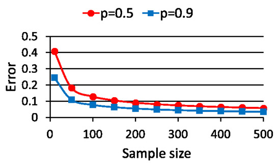
Figure 1. Error for sample size.

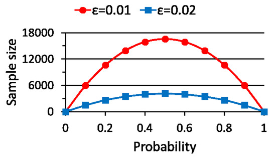
Figure 2. Sample size for probability.

Even if the value of $\widehat{p}(\mathit{x},\mathit{B})$ in (11) is unknown, the right side of the formula (11) takes its biggest value when $\widehat{p}(\mathit{x},\mathit{B})=0.5$. Therefore, the necessary sample size for SRS is obtained from (11) as

$${\displaystyle N\ge \frac{1}{4}{\left(\frac{z_{\delta /2}}{\epsilon }\right)}^2.}$$

(12)

Unfortunately, the sample size of SRS obtained theoretically by (12) is too large in practice. For example, the sample size in (12) becomes $N=\mathrm{16,587}$ for $\delta =0.01$ and $\epsilon =0.01$.

3.2. Weighted Stratified Sampling (WSS)

Since every sample ${\mathit{\xi }}^n\in \mathbf{\Xi }\subseteq \mathit{B}$ of SRS has the same probability of being chosen from the full data set $\mathit{B}$, few samples ${\mathit{\xi }}^n\in \mathbf{\Xi }$ are taken from the sparse part of $\mathit{B}$. In addition to the defect of SRS, the majority of data ${\mathit{\xi }}^{\ell }\in \mathit{B}$ are neglected by SRS even though the full data set $\mathit{B}$ is very large.

In order to use the full data set $\mathit{B}$ completely, we proposed a new data reduction method called WSS [17]. In the sampling technique called stratified sampling, which is often used in statistical survey [24], a data set is divided into some strata, or homogeneous subsets. This process is called stratification. Then, a few samples are selected from every stratum. Contrarily to clustering techniques used to divide a data set into some subsets [24], the stratification requires only “Internal cohesion” but not “External isolation”. Therefore, we can choose an arbitrary number of strata for WSS.

3.2.1. Procedure of WSS

A sample set $\mathbf{\Theta }\subseteq {\Re }^K$ is generated from the full data set $\mathit{B}\subseteq {\Re }^K$ as follows:

Step 1: 

By using a K-dimensional histogram, the full data set $\mathit{B}\subseteq {\Re }^K$ is divided exclusively into some strata ${\mathit{B}}_n\subseteq \mathit{B}$, $n=1,\cdots ,N$ as

$$\mathit{B}={\mathit{B}}_1\cup \cdots \cup {\mathit{B}}_n\cup \cdots \cup {\mathit{B}}_N$$

(13)

where ${\mathit{B}}_n\subseteq {\Re }^K$ and ${\mathit{B}}_n\ne \varnothing$, $n=1,\cdots ,N$.

Specifically, the K-dimensional histogram is a K-dimensional hypercube that contains the full data set $\mathit{B}\subseteq {\Re }^K$. On each side of the K-dimensional hypercube, the entire range of data is divided into a series of intervals. In this paper, the number of intervals is the same on all sides. Moreover, all intervals on each side have equal widths. Therefore, the K-dimensional histogram is an equi-width histogram [26]. Each bin of the K-dimensional histogram is also a K-dimensional hypercube. Then, nonempty bins are used to define strata ${\mathit{B}}_n\subseteq \mathit{B}$, $n=1,\cdots ,N$.

Step 2: 

A new sample point ${\mathit{\theta }}^n\in {\Re }^K$ is generated for each stratum ${\mathit{B}}_n\subseteq {\Re }^K$, $n=1,\cdots ,N$. Then, the sample set $\mathbf{\Theta }\subseteq {\Re }^K$ is defined as $\mathbf{\Theta }=\{{\mathit{\theta }}^1,\cdots ,{\mathit{\theta }}^n,\cdots ,{\mathit{\theta }}^N\}$.

Step 3: 

The weight $w_n\in \Re$ of each sample ${\mathit{\theta }}^n\in \mathbf{\Theta }$ is given by the size of ${\mathit{B}}_n$ as $w_n=\left|{\mathit{B}}_n\right|$.

By using a set of samples ${\mathit{\theta }}^n\in \mathbf{\Theta }$, $n=1,\cdots ,N$ and their weights $w_n\in \Re$ obtained by WSS, an empirical probability is calculated to approximate $\widehat{p}(\mathit{x},\mathit{B})$ in (4) as

$${\displaystyle \widehat{p}(\mathit{x},\mathbf{\Theta })=\frac{1}{W}\sum _{n=1}^N{w}_n\left(\prod _{m=1}^M\mathbb{𝟙}(g_m(\mathit{x},{\mathit{\theta }}^n)\le 0)\right)}$$

(14)

where $W=w_1+\cdots +w_n+\cdots +w_N$ and $w_n>0$, $n=1,\cdots ,N$.

3.2.2. Sample Generation by WSS

Each of the samples ${\mathit{\theta }}_n\in \mathbf{\Theta }$ of WSS is not necessary to be a sample from the stratum ${\mathit{B}}_n\subseteq \mathit{B}$. For generating samples ${\mathit{\theta }}_n\in \mathbf{\Theta }$, $n=1,\cdots ,N$ in Step 2, we think about the optimality of the sample set $\mathbf{\Theta }\subseteq {\Re }^K$. The best sample set $\mathbf{\Theta }\subseteq {\Re }^K$ minimizes the error metric of histogram [27] defined as

$${\displaystyle e_H(\mathbf{\Theta },\mathit{B})=\sum _{n=1}^N{e}_H({\mathit{\theta }}^n,{\mathit{B}}_n)=\sum _{n=1}^N\sum _{{\mathit{\xi }}^{\ell }\in {\mathit{B}}_n}{({\mathit{\theta }}^n-{\mathit{\xi }}^{\ell })}^2.}$$

(15)

In order to minimize the error metric of histogram in (15), we will solve the following differential equation about ${\mathit{\theta }}^n\in \mathbf{\Theta }$ because each term $e_H({\mathit{\theta }}^n,{\mathit{B}}_n)$ in (15) is convex.

$${\displaystyle \frac{\partial e_H({\mathit{\theta }}^n,{\mathit{B}}_n)}{\partial {\mathit{\theta }}^n}=2\left(|{\mathit{B}}_n|{\mathit{\theta }}^n-\sum _{{\mathit{\xi }}^{\ell }\in {\mathit{B}}_n}{\mathit{\xi }}^{\ell }\right)=0.}$$

(16)

By solving the differential equation in (16), we can obtain the optimal sample ${\mathit{\theta }}^n\in {\Re }^K$ as

$${\mathit{\theta }}^n=\frac{1}{|{\mathit{B}}_n|}\sum _{{\mathit{\xi }}^{\ell }\in {\mathit{B}}_n}{\mathit{\xi }}^{\ell }.$$

(17)

Consequently, in Step 2 of WSS, we have only to generate a new sample ${\mathit{\theta }}^n\in {\Re }^K$ by using the average point of all data ${\mathit{\xi }}^{\ell }\in {\mathit{B}}_n$ included in the stratum ${\mathit{B}}_n\subseteq \mathit{B}$ as shown in (17).

3.3. Relaxation Problems of CCP

As stated above, the equivalence problem of CCP in (5) is hard to solve. That is because the full data set $\mathit{B}$ is too large. Therefore, a data reduction method, namely SRS or WSS, is employed to formulate a relaxation problem of CCP. By using $\widehat{p}(\mathit{x},\mathbf{\Xi })$ in (6) or $\widehat{p}(\mathit{x},\mathbf{\Theta })$ in (14) to approximate $\widehat{p}(\mathit{x},\mathit{B})$ in (4), the relaxation problem of CCP is formulated as

$$\underset{\mathit{x}\in \mathit{X}}{min}f(\mathit{x})\mathrm{sub}.\mathrm{to}\widehat{p}(\mathit{x},\mathit{S})\ge \beta$$

(18)

where the sample set $\mathit{S}\subseteq {\Re }^K$ denotes either $\mathbf{\Xi }\subseteq {\Re }^K$ or $\mathbf{\Theta }\subseteq {\Re }^K$. The correction level $\beta \in (0,1]$ is chosen as $\beta \ge \alpha$ to compensate the margin of error $\epsilon \in (0,1)$ caused by SRS or WSS.

4. Adaptive Differential Evolution with Pruning Technique

Differential Evolution (DE) has been proven to be one of the most powerful global optimization algorithms [28,29]. Unfortunately, cardinal DE [18] is only applicable to unconstrained problems. Moreover, the performance of DE is significantly influenced by its control parameter settings. Therefore, in order to solve the relaxation problem of CCP shown in (18) efficiently, a new optimization method called Adaptive DE with Pruning technique (ADEP) is proposed. In the proposed ADEP, three techniques are introduced into cardinal DE [18]: (1) Adaptive control of parameters [19]; (2) Constraint handling based on feasibility rule [30]; and (3) Pruning technique in selection [17].

4.1. Strategy of DE

As well as cardinal DE [18], ADEP has a set of candidate solutions ${\mathit{x}}_i\in {\mathit{P}}_t$, $i=1,\cdots ,NP$ called population in each generation t. Each candidate solution ${\mathit{x}}_i\in \mathit{X}$ is a vector of decision variables. The initial population ${\mathit{x}}_i\in {\mathit{P}}_0\subseteq \mathit{X}$ is randomly generated according to a uniform distribution.

At each generation t, every ${\mathit{x}}_i\in {\mathit{P}}_t$ is assigned to a target vector in turn. By using the basic strategy of DE called “DE/rand/1/bin” [18], a trial vector ${\mathit{z}}_i\in \mathit{X}$ is generated from the target vector ${\mathit{x}}_i\in {\mathit{P}}_t$. Specifically, except for the current target vector ${\mathit{x}}_i\in {\mathit{P}}_t$, three other distinct vectors, say ${\mathit{x}}_{r1}$, ${\mathit{x}}_{r2}$, and ${\mathit{x}}_{r3}$, $i\ne r1\ne r2\ne r3$, are selected randomly from the population ${\mathit{P}}_t$. By using the three vectors, the differential mutation generates a new real vector ${\mathit{v}}_i\in {\Re }^D$ called mutated vector as

$${\mathit{v}}_i={\mathit{x}}_{r1}+F({\mathit{x}}_{r2}-{\mathit{x}}_{r3})$$

(19)

where $F\in [0.1,1]$ is a control parameter called scale factor.

The binomial crossover between the mutated vector ${\mathit{v}}_i\in {\Re }^D$ and the target vector ${\mathit{x}}_i\in {\mathit{P}}_t$ generates another real vector ${\mathit{z}}_i=(z_{1,i},\cdots ,z_{D,i})\in \mathit{X}$ called trial vector. Specifically, each component $z_{j,i}\in \Re$, $j=1,\cdots ,D$ of the trial vector ${\mathit{z}}_i\in \mathit{X}$ is inherited from either ${\mathit{v}}_i\in \mathit{X}$ or ${\mathit{x}}_i\in {\mathit{P}}_t$ as

$$z_{j,i}=\left\{\begin{array}{cc}{v}_{j,i}\hfill & \mathrm{if}{\mathrm{rand}}_j\le CR\vee j=j_r\hfill \\ x_{j,i}\hfill & \mathrm{otherwise}\hfill \end{array}\right.$$

(20)

where $CR\in [0,1]$ is a control parameter called crossover rate. ${\mathrm{rand}}_j\in [0,1]$ denotes a uniformly distributed random value. The subscript $j_r\in [1,D]$ is selected randomly every time, which ensures that the newborn vector ${\mathit{z}}_i\in \mathit{X}$ differs from the existing one ${\mathit{x}}_i\in {\mathit{P}}_t$ at least one element.

4.2. Adaptive Control of Parameters

The performance of DE depends on control parameters, namely the scale factor $F\in [0.1,1]$ in (19) and the crossover rate $CR\in [0,1]$ in (20). Therefore, various parameter adaptation mechanisms have been reported [28,29,31]. ADEP employs an adaptive parameter control mechanism in which feedback from the evolutionary search is used to dynamically change the control parameters [19].

According to the adaptive parameter control mechanism [19], all vectors ${\mathit{x}}_i\in {\mathit{P}}_t$, $i=1,\cdots ,NP$ have their own control parameters, namely $F_{i,t}\in [0.1,1]$ and $C{R}_{i,t}\in [0,1]$, at each generation t. Then, these control parameters are initialized as $F_{i,0}=0.5$ and $C{R}_{i,0}=0.9$, $i=1,\cdots ,NP$.

For generating the mutated vector ${\mathit{v}}_i\in {\Re }^D$ as shown in (19), the scale factor $F\in \Re$ is decided by using the control parameter $F_{i,t}\in [0.1,1]$ associated with the target vector ${\mathit{x}}_i\in {\mathit{P}}_t$ as

$$F=\left\{\begin{array}{cc}0.1+{\mathrm{rand}}_{1}0.9\hfill & \mathrm{if}{\mathrm{rand}}_2<0.1\hfill \\ F_{i,t}\hfill & \mathrm{otherwise}\hfill \end{array}\right.$$

(21)

where ${\mathrm{rand}}_j\in [0,1]$, $j=1,2$ are uniformly distributed values.

Similarly, for generating the trial vector ${\mathit{u}}_i\in {\Re }^D$ as shown in (20), the crossover rate $CR\in \Re$ is decided by using the control parameter $C{R}_{i,t}\in [0,1]$ associated with the target vector ${\mathit{x}}_i\in {\mathit{P}}_t$ as

$$CR=\left\{\begin{array}{cc}{\mathrm{rand}}_3\hfill & \mathrm{if}{\mathrm{rand}}_4<0.1\hfill \\ C{R}_{i,t}\hfill & \mathrm{otherwise}\hfill \end{array}\right.$$

(22)

where ${\mathrm{rand}}_j\in [0,1]$, $j=3,4$ are uniformly distributed values.

The trial vector ${\mathit{z}}_i\in \mathit{X}$ generated by using $F\in [0.1,1]$ in (21) and $CR\in [0,1]$ in (22) is compared with the target vector ${\mathit{x}}_i\in {\mathit{P}}_t$ as described below. If ${\mathit{z}}_i\in \mathit{X}$ is better than ${\mathit{x}}_i\in {\mathit{P}}_t$, ${\mathit{z}}_i\in \mathit{X}$ is selected for a new vector ${\mathit{x}}_i\in {\mathit{P}}_{t+1}$ of the next generation, and the control parameters of ${\mathit{x}}_i\in {\mathit{P}}_{t+1}$ are decided as $F_{i,t+1}=F$ and $C{R}_{i,t+1}=CR$. Otherwise, the target vector ${\mathit{x}}_i\in {\mathit{P}}_t$ survives to the next generation, and the control parameters of ${\mathit{x}}_i\in {\mathit{P}}_{t+1}$ are inherited from ${\mathit{x}}_i\in {\mathit{P}}_t$ as $F_{i,t+1}=F_{i,t}$ and $C{R}_{i,t+1}=C{R}_{i,t}$.

4.3. Constraint Handling and Pruning Technique in Selection

Evolutionary Algorithms (EAs) including DE are typically applied to problems in which bounds are the only constraints. Therefore, a number of Constraint Handling Techniques (CHTs) have been proposed in order to apply EAs to constrained optimization problems [32]. Among those CHTs, the feasibility rule [30] is one of the most widely used CHTs because of its simplicity and efficiency. Thus, ADEP uses a feasibility rule with the amount of constraint violation defined from (18) as

$$h({\mathit{x}}_i)=max\{\beta -\widehat{p}({\mathit{x}}_i,\mathit{S}),0\}$$

(23)

where the candidate solution ${\mathit{x}}_i\in {\mathit{P}}_t$ of CCP in (18) is feasible if $h({\mathit{x}}_i)=0$ holds.

At each generation t, the trial vector ${\mathit{z}}_i\in \mathit{X}$, $i=1,\cdots ,NP$ is compared with the corresponding target vector ${\mathit{x}}_i\in {\mathit{P}}_t$. Then, either the trial vector ${\mathit{z}}_i\in \mathit{X}$ or the target vector ${\mathit{x}}_i\in {\mathit{P}}_t$ is selected for a vector ${\mathit{x}}_i\in {\mathit{P}}_{t+1}$ of the next generation. First of all, if the following condition is satisfied,

$$(h({\mathit{x}}_i)=0)\wedge (f({\mathit{x}}_i)<f({\mathit{z}}_i))$$

(24)

the trial vector ${\mathit{z}}_i\in \mathit{X}$ is discarded immediately because ${\mathit{x}}_i\in {\mathit{P}}_t$ is better than ${\mathit{z}}_i\in \mathit{X}$. Then, the trial vector ${\mathit{x}}_i\in {\mathit{P}}_t$ survives to the next generation. Since the pruning technique based on the condition in (24) does not require the value of $h({\mathit{z}}_i)$, it is very effective to reduce the run time of ADEP.

Only when the condition in (24) is not satisfied, the probability $\widehat{p}({\mathit{z}}_i,\mathit{S})$ is evaluated by using the sample set $\mathit{S}\subseteq {\Re }^K$ to get the value of $h({\mathit{z}}_i)$. If either of the following conditions is satisfied,

$$\left[\begin{array}{c}h({\mathit{z}}_i)<h({\mathit{x}}_i)\hfill \\ (h({\mathit{z}}_i)=h({\mathit{x}}_i))\wedge (f({\mathit{z}}_i)\le f({\mathit{x}}_i))\hfill \end{array}\right.$$

(25)

the trial vector ${\mathit{z}}_i\in \mathit{X}$ is selected for a new vector ${\mathit{x}}_i\in {\mathit{P}}_{t+1}$ of the next generation. Otherwise, the current target vector ${\mathit{x}}_i\in {\mathit{P}}_t$ survives to the next generation and becomes a vector ${\mathit{x}}_i\in {\mathit{P}}_{t+1}$.

4.4. Proposed Algorithm of ADEP

The algorithm of ADEP is described as follows. The maximum number of generations $NT$ is given as the termination condition. The population size $NP$ is chosen as $NP=5D$ [18].

Step 1: 

Randomly generate the initial population ${\mathit{x}}_i\in {\mathit{P}}_0\subseteq \mathit{X}$, $i=1,\cdots ,NP$. $t=0$.

Step 2: 

For $i=1$ to $NP$, evaluate $f({\mathit{x}}_i)$ and $h({\mathit{x}}_i)$ for each vector ${\mathit{x}}_i\in {\mathit{P}}_0$.

Step 3: 

If $t=NT$ holds, output the best solution ${\mathit{x}}_b\in {\mathit{P}}_t$ and terminate ADEP.

Step 4: 

For $i=1$ to $NP$, generate the trial vector ${\mathit{z}}_i\in \mathit{X}$ from the target vector ${\mathit{x}}_i\in {\mathit{P}}_t$.

Step 5: 

For $i=1$ to $NP$, evaluate $f({\mathit{z}}_i)$ for the trial vector ${\mathit{z}}_i\in \mathit{X}$.

Step 6: 

For $i=1$ to $NP$, evaluate $h({\mathit{z}}_i)$ for ${\mathit{z}}_i\in \mathit{X}$ only if the condition in (24) is not satisfied.

Step 7: 

For $i=1$ to $NP$, select either ${\mathit{z}}_i\in \mathit{X}$ or ${\mathit{x}}_i\in {\mathit{P}}_t$ for ${\mathit{x}}_i\in {\mathit{P}}_{t+1}$. $t=t+1$.

Step 8: 

Go back to Step 3.

5. Performance Evaluation of WSS

We evaluate the performance of the proposed WSS by comparison with the conventional SRS. Specifically, by using WSS and SRS, we estimate the probability meeting $g(\mathit{x},{\mathit{\xi }}^{\ell })\le \gamma$ as

$${\displaystyle \widehat{p}(\mathit{x},\mathit{B})=\frac{1}{\left|\mathit{B}\right|}\sum _{{\mathit{\xi }}^{\ell }\in \mathit{B}}\mathbb{𝟙}(g(\mathit{x},{\mathit{\xi }}^{\ell })\le \gamma )}$$

(26)

where $g:\mathit{X}\times \mathbf{\Omega }\to \Re$ is a measurable function.

From (9) to (11), the performance of SRS depends on the value of the probability $\widehat{p}(\mathit{x},\mathit{B})$ to be estimated. Therefore, by changing the value of $\gamma \in \Re$ in (26), we change the value of the probability to be estimated by SRS and WSS. From a full data set $\mathit{B}\subseteq {\Re }^K$, the sample sets $\mathbf{\Xi }\subseteq {\Re }^K$ and $\mathbf{\Theta }\subseteq {\Re }^K$ are generated, respectively, by using SRS and WSS. Then, the estimation error is defined as

$${\epsilon }_p(\mathit{S},\mathit{B})=|\widehat{p}(\mathit{x},\mathit{S})-\widehat{p}(\mathit{x},\mathit{B})|$$

(27)

where the sample set $\mathit{S}\subseteq {\Re }^K$ denotes either $\mathbf{\Xi }\subseteq {\Re }^K$ or $\mathbf{\Theta }\subseteq {\Re }^K$.

5.1. Case Study 1

Each value ${\xi }_i\in \Re$ of practical data $\mathit{\xi }\in \mathbf{\Omega }$ in (2) usually has a range. Therefore, a full data set ${\mathit{\xi }}^{\ell }=({\xi }_1,{\xi }_2)\in \mathit{B}\subseteq {\Re }^2$ is generated randomly by using a truncated normal distribution as

$${\xi }_j\sim \mathcal{N}({\mu }_j,{\sigma }_j^2,{\mu }_j-3{\sigma }_j,{\mu }_j+3{\sigma }_j),j=1,2$$

(28)

where the mean is $\mathit{\mu }=({\mu }_1,{\mu }_2)=(1,2)$ and the variance is ${\mathit{\sigma }}^2=({\sigma }_1^2,{\sigma }_2^2)=({0.1}^2,{0.2}^2)$.

The truncated normal distribution in (28) is the probability distribution derived from that of a normally distributed random variable by bounding the random variable as ${\xi }_j\in [{\mu }_j-3{\sigma }_j,{\mu }_j+3{\sigma }_j]$. The correlation matrix of the random variables ${\xi }_j\in \Re$, $j=1,2$ is also given as

$$\mathit{R}=\left(\begin{array}{ccc}1.0& & {\rho }_{12}\\ {\rho }_{21}& & 1.0\end{array}\right)=\left(\begin{array}{ccc}\hfill 1.0& & \hfill -0.8\\ \hfill -0.8& & \hfill 1.0\end{array}\right).$$

(29)

Please notice that the full data set ${\mathit{\xi }}^{\ell }\in \mathit{B}$ is i.i.d. even if the elements of ${\mathit{\xi }}^{\ell }\in \mathit{B}$ have a correlation. The size of the full data set $\mathit{B}\subseteq {\Re }^2$ generated randomly is $\left|\mathit{B}\right|={10}^7$. Figure 3 shows the spatial patterns of the full data ${\mathit{\xi }}^{\ell }\in \mathit{B}$ and the random samples ${\mathit{\xi }}^n\in \mathbf{\Xi }\subseteq \mathit{B}$, $n=1,\cdots ,N$ selected by SRS. Figure 4 also shows the full data ${\mathit{\xi }}^{\ell }\in \mathit{B}$ and the weighted samples ${\mathit{\theta }}^n\in \mathbf{\Theta }$ generated by WSS.

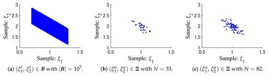
Figure 3. Patterns of the full data ${\mathit{\xi }}^{\ell }\in \mathit{B}\subseteq {\Re }^2$ and the random samples ${\mathit{\xi }}^n\in \mathbf{\Xi }$ selected by SRS.

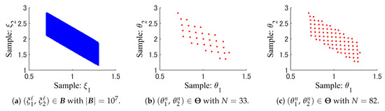
Figure 4. Patterns of the full data ${\mathit{\xi }}^{\ell }\in \mathit{B}\subseteq {\Re }^2$ and the weighted samples ${\mathit{\theta }}^n\in \mathbf{\Theta }$ generated by WSS.

From Figure 3 and Figure 4, we can see that the weighted samples ${\mathit{\theta }}^n\in \mathbf{\Theta }$, $n=1,\cdots ,N$ of WSS are scattered more widely as compared to the random samples ${\mathit{\xi }}^n\in \mathbf{\Xi }$ of SRS. Especially, SRS has not taken any samples ${\mathit{\xi }}^n\in \mathbf{\Xi }$ from the sparse part of the full data set $\mathit{B}\subseteq {\Re }^2$ in Figure 3.

For the probability $\widehat{p}(\mathit{x},\mathit{B})$ in (26), a function $g(\mathit{x},{\mathit{\xi }}^{\ell })$ is defined as

$${\displaystyle g(\mathit{x},{\mathit{\xi }}^{\ell })=\frac{x_1{\xi }_1+x_2{\xi }_2}{2}=\frac{{\xi }_1+{\xi }_2}{2}}$$

(30)

where the vector of decision variables is given as $\mathit{x}=(x_1,x_2)=(1,1)$.

The probability in (26) becomes $\widehat{p}(\mathit{x},\mathit{B})\simeq 0.933$ when $\gamma =1.6$ is chosen. Then, the estimation errors in (27), namely ${\epsilon }_p(\mathbf{\Theta },\mathit{B})$ and ${\epsilon }_p(\mathbf{\Xi },\mathit{B})$, are evaluated 100 times for each sample size by using different full data sets $\mathit{B}\subseteq {\Re }^2$ and summarized in Figure 5. From Figure 5, the average value and the standard deviation of ${\epsilon }_p(\mathbf{\Theta },\mathit{B})$ are smaller than those of ${\epsilon }_p(\mathbf{\Xi },\mathit{B})$ for any sample sizes. Furthermore, ${\epsilon }_p(\mathbf{\Theta },\mathit{B})$ converges to almost zero faster than ${\epsilon }_p(\mathbf{\Xi },\mathit{B})$ on average. Consequently, we can say that the proposed WSS outperforms the conventional SRS in the accuracy of the estimated probability.

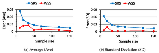
Figure 5. Estimation error for sample size when $\widehat{p}(\mathit{x},\mathit{B})\simeq 0.933$ ($K=2$).

The probability in (26) becomes $\widehat{p}(\mathit{x},\mathit{B})\simeq 0.773$ when $\gamma =1.55$ is chosen. The estimation errors in (27) are evaluated for WSS and SRS with the probability $\widehat{p}(\mathit{x},\mathit{B})\simeq 0.773$ as stated above and summarized in Figure 6. The probability in (26) becomes $\widehat{p}(\mathit{x},\mathit{B})\simeq 0.500$ when $\gamma =1.5$ is chosen. The estimation errors in (27) are also evaluated for WSS and SRS with the probability $\widehat{p}(\mathit{x},\mathit{B})\simeq 0.500$ and summarized in Figure 7. From Figure 6 and Figure 7, the standard deviation of ${\epsilon }_p(\mathbf{\Theta },\mathit{B})$ is always smaller than that of ${\epsilon }_p(\mathbf{\Xi },\mathit{B})$. On the other hand, in the average value of the estimation errors, WSS seems to lose the advantage over SRS when the probability value gets closer to $\widehat{p}(\mathit{x},\mathit{B})=0.5$.

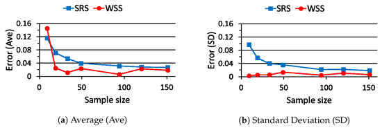
Figure 6. Estimation error for sample size when $\widehat{p}(\mathit{x},\mathit{B})\simeq 0.773$ ($K=2$).

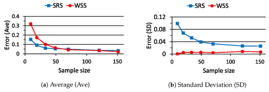
Figure 7. Estimation error for sample size when $\widehat{p}(\mathit{x},\mathit{B})\simeq 0.500$ ($K=2$).

From Figure 5, Figure 6 and Figure 7, the performance of WSS depends not only on the sample size but also on the probability value to be estimated. Then, WSS outperforms SRS when the probability value is large. A large value is usually chosen for the probability meeting all constraints in CCP. Consequently, we can say that WSS is more suitable for formulating the relaxation problem of CCP in (18).

5.2. Case Study 2

A full data set ${\mathit{\xi }}^{\ell }=({\xi }_1,{\xi }_2,{\xi }_3)\in \mathit{B}\subseteq {\Re }^3$ is generated randomly as

$${\xi }_j\sim \mathcal{N}({\mu }_j,{\sigma }_j^2,{\mu }_j-3{\sigma }_j,{\mu }_j+3{\sigma }_j),j=1,2,3$$

(31)

where $\mathit{\mu }=({\mu }_1,{\mu }_2,{\mu }_3)=(1.5,2.0,1.0)$ and ${\mathit{\sigma }}^2=({\sigma }_1^2,{\sigma }_2^2,{\sigma }_3^2)=({0.2}^2,{0.1}^2,{0.1}^2)$.

The correlation matrix of the random variables ${\xi }_j\in \Re$, $j=1,2,3$ is also given as

$$\begin{array}{ccccc}\mathit{R}& =& \left(\begin{array}{ccc}1.0& {\rho }_{12}& {\rho }_{13}\\ {\rho }_{21}& 1.0& {\rho }_{23}\\ {\rho }_{31}& {\rho }_{32}& 1.0\end{array}\right)& =& \left(\begin{array}{ccc}\hfill 1.0& \hfill 0.6& \hfill 0.0\\ \hfill 0.6& \hfill 1.0& \hfill -0.4\\ \hfill 0.0& \hfill -0.4& \hfill 1.0\end{array}\right).\end{array}$$

(32)

The size of the full data set $\mathit{B}\subseteq {\Re }^3$ generated randomly is $\left|\mathit{B}\right|={10}^7$. Figure 8 shows the spatial patterns of the full data ${\mathit{\xi }}^{\ell }\in \mathit{B}$ and the random samples ${\mathit{\xi }}^n\in \mathbf{\Xi }\subseteq \mathit{B}$, $n=1,\cdots ,N$ selected by SRS. Figure 9 also shows the full data ${\mathit{\xi }}^{\ell }\in \mathit{B}$ and the weighted samples ${\mathit{\theta }}^n\in \mathbf{\Theta }$ generated by WSS.

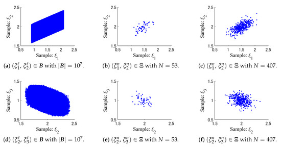
Figure 8. Patterns of the full data ${\mathit{\xi }}^{\ell }\in \mathit{B}\subseteq {\Re }^3$ and the random samples ${\mathit{\xi }}^n\in \mathbf{\Xi }$ selected by SRS.

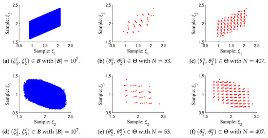
Figure 9. Patterns of the full data ${\mathit{\xi }}^{\ell }\in \mathit{B}\subseteq {\Re }^3$ and the weighted samples ${\mathit{\theta }}^n\in \mathbf{\Theta }$ generated by WSS.

From Figure 8 and Figure 9, we can see that the weighted samples ${\mathit{\theta }}^n\in \mathbf{\Theta }$, $n=1,\cdots ,N$ of WSS are scattered more widely than the random samples ${\mathit{\xi }}^n\in \mathbf{\Xi }$ of SRS. Some weighted samples ${\mathit{\theta }}^n\in \mathbf{\Theta }$ shown in Figure 9 seem to be overlapped each other due to the high dimensionality $K=3$ of them. However, we can recognizable the uniformity in the pattern of the weighted samples ${\mathit{\theta }}^n\in \mathbf{\Theta }$.

For the probability $\widehat{p}(\mathit{x},\mathit{B})$ in (26), a linear function $g(\mathit{x},{\mathit{\xi }}^{\ell })$ is defined as

$${\displaystyle g(\mathit{x},{\mathit{\xi }}^{\ell })=\frac{x_1{\xi }_1+x_2{\xi }_2+x_3{\xi }_3}{3}=\frac{{\xi }_1+{\xi }_2+{\xi }_3}{3}}$$

(33)

where the vector of decision variables is given as $\mathit{x}=(x_1,x_2,x_3)=(1,1,1)$.

The probability in (26) becomes $\widehat{p}(\mathit{x},\mathit{B})\simeq 0.986$ when $\gamma =1.7$ is chosen. Then, the estimation errors in (27), namely ${\epsilon }_p(\mathbf{\Theta },\mathit{B})$ and ${\epsilon }_p(\mathbf{\Xi },\mathit{B})$, are evaluated 100 times for each sample size by using different full data sets $\mathit{B}\subseteq {\Re }^3$ and summarized in Figure 10. From Figure 10, the average value and the standard deviation of ${\epsilon }_p(\mathbf{\Theta },\mathit{B})$ are smaller than those of ${\epsilon }_p(\mathbf{\Xi },\mathit{B})$ for any sample sizes. From these results, we confirm that the proposed WSS outperforms the conventional SRS in this case.

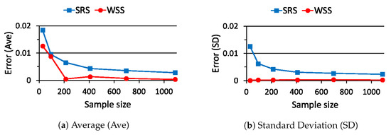
Figure 10. Estimation error for sample size with the linear function in (33).

5.3. Case Study 3

A full data set $\mathit{B}\subseteq {\Re }^3$, $\left|\mathit{B}\right|={10}^7$ is generated randomly as shown in (31) and (32). For the probability $\widehat{p}(\mathit{x},\mathit{B})$ in (26), a non-linear function $g(\mathit{x},{\mathit{\xi }}^{\ell })$ is defined as

$${\displaystyle g(\mathit{x},{\mathit{\xi }}^{\ell })=\frac{x_1{\xi }_1^2+x_2{\xi }_2^2+x_3{\xi }_3^2}{3}=\frac{{\xi }_1^2+{\xi }_2^2+{\xi }_3^2}{3}}$$

(34)

where the vector of decision variables is given as $\mathit{x}=(x_1,x_2,x_3)=(1,1,1)$.

The probability in (26) becomes $\widehat{p}(\mathit{x},\mathit{B})\simeq 0.817$ when $\gamma =1.7$ is chosen. The estimation errors in (27) are evaluated for WSS and SRS with the probability $\widehat{p}(\mathit{x},\mathit{B})\simeq 0.817$ as stated above and summarized in Figure 11. From Figure 11, WSS is also better than SRS because the average value and the standard deviation of ${\epsilon }_p(\mathbf{\Theta },\mathit{B})$ are smaller than those of ${\epsilon }_p(\mathbf{\Xi },\mathit{B})$ for any sample sizes.

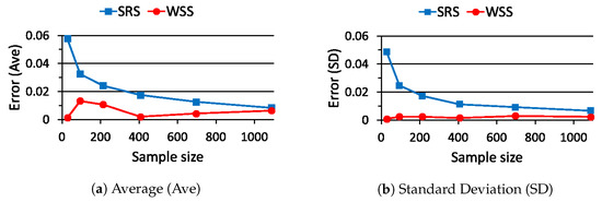
Figure 11. Estimation error for sample size with the non-linear function in (34).

From Figure 10 and Figure 11, we can see that the margin of error provided by WSS converges fast, and then it does not decrease even if the sample size is increased. Therefore, WSS can estimate the probability accurately with a small sample size if we choose the sample size properly.

6. Flood Control Planning

6.1. Formulation of CCP

Reservoirs are constructed to protect an urban area at the lower part of river from the flood damage caused by torrential rain. The flood control reservoir system design has been formulated as CCP [33]. In addition to the reservoir, the water-retaining capacity of forest is counted to prevent the flood caused by heavy rainfall. Thereby, the flood control planning is formulated as CCP [5].

Figure 12 shows a topological river model. Symbol ◯ denotes a forest considered in the flood control planning. There are three forests in watersheds. The gross area of each forest $a_j$, $j=1,2,3$ is a constant. The amount of rainfall ${\xi }_j\in \Re$ per unit area in each of the forests is a random variable. The water-retaining capacity of forest $x_j\in \Re$, $j=1,2,3$ per unit area is regarded as a decision variable because it can be controlled through the forest maintenance such as afforestation. According to the model of the forest mechanism [34], the inflow of water $q_j\in \Re$ from each forest to the river is

$$q_j(x_j,{\xi }_j)=a_j({\xi }_j-x_j(1-exp(-{\xi }_j/x_j)))$$

(35)

where the effect of past rainfall is not considered in the model [34].

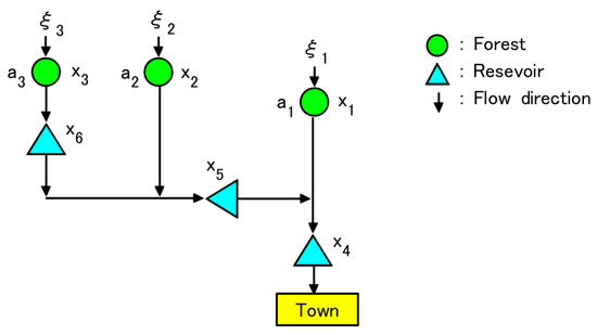
Figure 12. Topological river model.

Symbol △ in Figure 12 denotes a reservoir. Three reservoirs are constructed in the river. The capacity of each reservoir $x_j\in \Re$, $j=4,5,6$ is also a decision variable. From $q_j(x_j,{\xi }_j)\in \Re$ in (35), the inflow of water from the river to the town located at the lower part of the river is calculated as

$$g(\mathit{x},\mathit{\xi })=max\{max\{max\{q_3-x_6,0\}+q_2-x_5,0\}+q_1-x_4,0\}$$

(36)

where $q_j\in \Re$, $j=1,2,3$ denotes $q_j(x_j,{\xi }_j)\in \Re$ defined by (35).

The probability of meeting $g(\mathit{x},\mathit{\xi })\le 0$ has to be greater than $\alpha \in (0,1)$. The maintenance cost of a forest is proportional to its capacity. The construction cost of a reservoir is proportional to the square of its capacity. Then, the flood control planning to minimize the total cost is formulated as

$$\left[\begin{array}{ccc}{\displaystyle \underset{\mathit{x}\in \mathit{X}}{min}}\hfill & & {\displaystyle f(\mathit{x})=\sum _{j=1}^3{a}_j{x}_j+\sum _{j=4}^6{x}_j^2}\hfill \\ \mathrm{sub}.\mathrm{to}\hfill & & Pr\left(\forall \mathit{\xi }\in \mathbf{\Omega }:g_m(\mathit{x},\mathit{\xi })\le 0,m=1,2,3\right)\ge \alpha \hfill \\ \hfill & & 0.5\le x_1\le 1.5,0.5\le x_2\le 1.5,0.5\le x_3\le 1.5,\hfill \\ \hfill & & 0\le x_4\le 3,0\le x_5\le 3,0\le x_6\le 4\hfill \end{array}\right.$$

(37)

where $a_j=2$, $j=1,2,3$. From (36), functions $g_m(\mathit{x},\mathit{\xi })$, $m=1,2,3$ are derived as

$$\left[\begin{array}{ccc}\hfill g_1(\mathit{x},\mathit{\xi })& =& q_1(x_1,{\xi }_1)-x_4\hfill \\ \hfill g_2(\mathit{x},\mathit{\xi })& =& q_1(x_1,{\xi }_1)+q_2(x_2,{\xi }_2)-x_4-x_5\hfill \\ \hfill g_3(\mathit{x},\mathit{\xi })& =& q_1(x_1,{\xi }_1)+q_2(x_2,{\xi }_2)+q_3(x_3,{\xi }_3)-x_4-x_5-x_6.\hfill \end{array}\right.$$

(38)

6.2. Comparison of SRS and WSS

We suppose that the amount of rainfall $\mathit{\xi }\in \mathbf{\Omega }$ in (37) is given as “big data”. For convenience, the full data set ${\mathit{\xi }}^{\ell }=({\xi }_1,{\xi }_2,{\xi }_3)\in \mathit{B}\subseteq \mathbf{\Omega }$ is generated randomly by using the truncated normal distribution shown in (31). Please notice that ${\mathit{\xi }}^{\ell }\in \mathit{B}$ denotes the amount of rainfall in one period, but the river flow depending on an actual time. The inflow of water $q_j\in \Re$ is derived from ${\xi }_j\in \Re$ as shown in (35). Therefore, the full data set ${\mathit{\xi }}^{\ell }\in \mathit{B}$ is i.i.d. On the other hand, a set of ${\xi }_j\in \Re$, $j=1,2,3$ is not i.i.d. The correlation matrix of the amounts of rainfalls ${\xi }_j\in \Re$, $j=1,2,3$ is given as

$$\begin{array}{ccccc}\mathit{R}& =& \left(\begin{array}{ccc}1.0& {\rho }_{12}& {\rho }_{13}\\ {\rho }_{21}& 1.0& {\rho }_{23}\\ {\rho }_{31}& {\rho }_{32}& 1.0\end{array}\right)& =& \left(\begin{array}{ccc}\hfill 1.0& \hfill 0.5& \hfill 0.0\\ \hfill 0.5& \hfill 1.0& \hfill 0.3\\ \hfill 0.0& \hfill 0.3& \hfill 1.0\end{array}\right).\end{array}$$

(39)

The size of the full data set $\mathit{B}\subseteq {\Re }^3$ generated randomly is $\left|\mathit{B}\right|={10}^7$. Figure 13 shows the spatial patterns of the full data ${\mathit{\xi }}^{\ell }\in \mathit{B}$, the random samples ${\mathit{\xi }}^n\in \mathbf{\Xi }\subseteq \mathit{B}$, $n=1,\cdots ,N$ selected by SRS, and the weighted samples ${\mathit{\theta }}^n\in \mathbf{\Theta }$, $n=1,\cdots ,N$ generated by WSS.

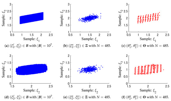
Figure 13. Patterns of the full data set, the random samples of SRS, and the weighted samples of WSS.

From Figure 13, we can see that the weighted samples ${\mathit{\theta }}^n\in \mathbf{\Theta }$, $n=1,\cdots ,N$ of WSS are scattered more widely than the random samples ${\mathit{\xi }}^n\in \mathbf{\Xi }$, $n=1,\cdots ,N$ of SRS. Some weighted samples ${\mathit{\theta }}^n\in \mathbf{\Theta }$ of WSS seem to be overlapped each other in Figure 13 due to the high dimensionality $K=3$ of them. However, we can recognizable the uniformity in the pattern of the weighted samples ${\mathit{\theta }}^n\in \mathbf{\Theta }$.

The flood control planning formulated as CCP in (37) is transformed into an equivalence problem of CCP as shown in (5) by using the above full data set $\mathit{B}\subseteq {\Re }^3$, $\left|\mathit{B}\right|={10}^7$. For a solution $\mathit{x}\in \mathit{X}$ of the equivalence problem of CCP, the joint probability defined by (4) and (37) becomes $\widehat{p}(\mathit{x},\mathit{B})\simeq 0.906$. By using SRS and WSS respectively, we estimate the value of the joint probability $\widehat{p}(\mathit{x},\mathit{B})$.

The estimation errors in (27), namely ${\epsilon }_p(\mathbf{\Theta },\mathit{B})$ and ${\epsilon }_p(\mathbf{\Xi },\mathit{B})$, are evaluated 100 times for each sample size by using different full data sets $\mathit{B}\subseteq {\Re }^3$ and summarized in Figure 14. From Figure 14, the average value and the standard deviation of ${\epsilon }_p(\mathbf{\Theta },\mathit{B})$ are smaller than those of ${\epsilon }_p(\mathbf{\Xi },\mathit{B})$ for any sample sizes. From these results, we confirm that WSS outperforms SRS in this case too.

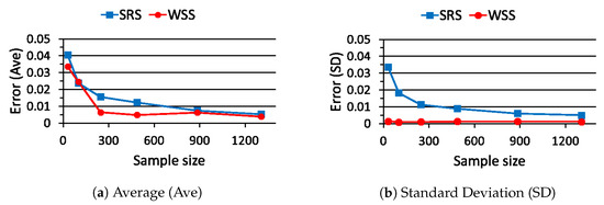
Figure 14. Estimation error for sample size in the flood control planning.

6.3. Solution of CCP

By using the weighted samples ${\mathit{\theta }}^n\in \mathbf{\Theta }$, $n=1,\cdots ,N$ of WSS, the flood control planning formulated as CCP in (37) is transformed into a relaxation problem of CCP as shown in (18). That is because the result in Figure 14 shows that WSS estimates the value of $\widehat{p}(\mathit{x},\mathit{B})$ using fewer samples than SRS. From the average value of ${\epsilon }_p(\mathbf{\Theta },\mathit{B})$ in Figure 14, the sample size is chosen as $N\simeq 482$.

The proposed ADEP is coded in MATLAB [35]. The parameters of ADEP and WSS are chosen as shown in Table 1. As stated above, the sample size is chosen as $N\simeq 482$. For a sufficiency level $\alpha \in (0,1)$ in (37), the correction level in (18) is chosen as $\beta =\alpha +0.03$. The population size is decided as $NP=5D$ by recommendation of the literature [18]. The maximum number of generations is decided as $NT=80$ through a preliminary experiment. Figure 15 shows the convergence graph of ADEP when the sufficiency level is chosen as $\alpha =0.9$ or $\alpha =0.6$. The horizontal axis of Figure 15 is the number of generations. The vertical axis is the best objective function value achieved at each generation. From Figure 15, we can confirm that $NT=80$ is a sufficiently large number of generations.

Table 1. Parameters of ADEP and WSS for the relaxation problem of CCP.

Generation: $\mathit{NT}$	Population Size: $\mathit{NP}$	Sample Size: N	Correction Level: $\mathit{\beta }$
80	30	482	$\alpha +0.03$

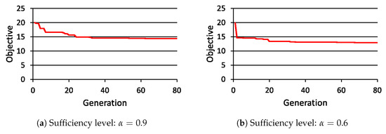
Figure 15. Convergence graph of ADEP.

ADEP is applied to the relaxation problem of CCP 50 times. For the respective runs of ADEP, different full data sets $\mathit{B}\subseteq {\Re }^3$ and initial populations ${\mathit{P}}_0\subseteq \mathit{X}$ are generated randomly. Every solution ${\mathit{x}}_b\in \mathit{X}$ obtained by ADEP for the relaxation problem of CCP is checked whether it also satisfies the constraint of the equivalence problem of CCP. From the ratio of the infeasible solutions ${\mathit{x}}_b\in \mathit{X}$ that do not meet the constraint $\widehat{p}({\mathit{x}}_b,\mathit{B})\ge \alpha$, the risk of failure $\delta \in (0,1)$ in (8) is evaluated empirically.

Table 2 shows the results of the experiments conducted for several sufficiency levels $\alpha \in (0,1)$ in which $f({\mathit{x}}_b)$ denotes the objective function value of the best solution ${\mathit{x}}_b\in \mathit{X}$ obtained by ADEP for a given $\alpha \in (0,1)$; $\widehat{p}({\mathit{x}}_b,\mathbf{\Theta })$ and $\widehat{p}({\mathit{x}}_b,\mathit{B})$ are empirical probabilities provided by ${\mathit{x}}_b\in \mathit{X}$; ${\epsilon }_p(\mathbf{\Theta },\mathit{B})$ is the estimation error defined by (27); $\widehat{\delta }\in [0,1]$ is the risk of failure evaluated empirically as stated above. Except the risk of failure $\widehat{\delta }\in [0,1]$, the results in Table 2 are averaged over 50 runs.

Table 2. Solutions obtained by ADEP for CCP in (37).

$\mathit{\alpha }$	$\mathit{\beta }$	$\mathit{f}({\mathit{x}}_{\mathit{b}})$	$\widehat{\mathit{p}}({\mathit{x}}_{\mathit{b}},\mathbf{\Theta })$	$\widehat{\mathit{p}}({\mathit{x}}_{\mathit{b}},\mathit{B})$	${\mathit{\epsilon }}_{\mathit{p}}(\mathbf{\Theta },\mathit{B})$	$\widehat{\mathit{\delta }}$
$0.9$	$0.93$	$14.438$	$0.934$	$0.921$	$0.012$	$0.00$
$0.8$	$0.83$	$13.725$	$0.837$	$0.809$	$0.028$	$0.00$
$0.7$	$0.73$	$13.355$	$0.737$	$0.725$	$0.012$	$0.00$
$0.6$	$0.63$	$12.949$	$0.636$	$0.609$	$0.027$	$0.16$

From Table 2, we can confirm the usefulness of the proposed method. Even though the sample size N of WSS is small, the value of $\widehat{p}({\mathit{x}}_b,\mathbf{\Theta })$ is very close to $\widehat{p}({\mathit{x}}_b,\mathit{B})$, and ${\epsilon }_p(\mathbf{\Theta },\mathit{B})<0.03$ holds for every $\alpha \in (0,1)$. Moreover, the majority of the solutions ${\mathit{x}}_b\in \mathit{X}$ satisfy the constraint $\widehat{p}({\mathit{x}}_b,\mathit{B})\ge \alpha$. Therefore, if we suppose that $\widehat{p}({\mathit{x}}_b,\mathit{B})\simeq p({\mathit{x}}_b,\mathbf{\Omega })$ holds, the solution ${\mathit{x}}_b\in \mathit{X}$ is regarded as a feasible solution of CCP in (37). We also see the trade-off between the optimality of the solution ${\mathit{x}}_b\in \mathit{X}$ evaluated by $f({\mathit{x}}_b)$ and the reliability specified by $\alpha \in (0,1)$. From the value of $\widehat{\delta }\in [0,1]$, it seems to be hard to obtain feasible solutions of CCP in (37) for a small sufficiency level: $\alpha =0.6$. That is because WSS is suitable for estimating a large value of $\widehat{p}({\mathit{x}}_b,\mathit{B})$ as shown in Figure 5, Figure 6 and Figure 7.

7. Performance Evaluation of ADEP

For solving the relaxation problem of CCP efficiently, the pruning technique shown in (24) is introduced into an Adaptive DE (ADE) and ADEP is proposed. By comparing ADE with ADEP, the ability of the pruning technique to reduce the run time of ADE is evaluated. The flood control planning formulated as CCP in (37) is used to draw a comparison between ADE and ADEP. Therefore, the control parameters of them are given by Table 1 except the sampe size N. Thereby, ADE and ADEP are executed on a personal computer (CPU: Intel(R) Core(TM) i7-3770@3.40GHz, Memory: 16.0GB).

By changing the value of $\beta \in (0,1)$ with a sample size $N\simeq 482$, ADE and ADEP are applied to the relaxation problem of CCP, respectively, 50 times. Table 3 shows the results of the experiments average over 50 runs in which $f({\mathit{x}}_b)$ is the objective function value of the best solution ${\mathit{x}}_b\in \mathit{X}$; $\widehat{p}({\mathit{x}}_b,\mathbf{\Theta })$ is the empirical probability provided by ${\mathit{x}}_b\in \mathit{X}$. The run time of each algorithm except the generation of the full data set $\mathit{B}\subseteq {\Re }^3$, $\left|\mathit{B}\right|={10}^7$ is also shown in Table 3. Rate in Table 3 means the percentage of the trial vectors ${\mathit{z}}_i\in \mathit{X}$ which are discarded by the pruning technique used in ADEP. Furthermore, the numbers in parenthesis indicate the standard deviations of the respective values in Table 3.

Table 3. Comparison between ADE and ADEP with sample size $N\simeq 482$.

	ADE			ADEP
$\mathit{\beta }$	$\mathit{f}({\mathit{x}}_{\mathit{b}})$	$\widehat{\mathit{p}}({\mathit{x}}_{\mathit{b}},\mathbf{\Theta })$	Time [s]	$\mathit{f}({\mathit{x}}_{\mathit{b}})$	$\widehat{\mathit{p}}({\mathit{x}}_{\mathit{b}},\mathbf{\Theta })$	Time [s]	Rate
$0.93$	$14.438$	$0.934$	$0.263$	$14.438$	$0.934$	$0.189$	$0.509$
	($0.035$)	($0.001$)	($0.023$)	($0.035$)	($0.001$)	($0.013$)	($0.015$)
$0.83$	$13.725$	$0.837$	$0.267$	$13.725$	$0.837$	$0.190$	$0.514$
	($0.034$)	($0.002$)	($0.011$)	($0.034$)	($0.002$)	($0.010$)	($0.013$)
$0.73$	$13.355$	$0.737$	$0.263$	$13.355$	$0.737$	$0.186$	$0.521$
	($0.032$)	($0.009$)	($0.015$)	($0.032$)	($0.009$)	($0.012$)	($0.015$)
$0.63$	$12.949$	$0.636$	$0.265$	$12.949$	$0.636$	$0.185$	$0.519$
	($0.032$)	($0.009$)	($0.018$)	($0.032$)	($0.009$)	($0.009$)	($0.013$)

From Table 3, we confirm that the pruning technique works well for reducing the run time of ADEP. Besides, the high rate in Table 3 shows that more than half of the trial vectors ${\mathit{z}}_i\in \mathit{X}$ are eliminated by the pruning technique without evaluating the value of $h({\mathit{z}}_i)$ in (23). From the values of $f({\mathit{x}}_b)$ and $\widehat{p}({\mathit{x}}_b,\mathbf{\Theta })$ in Table 3, we can also see that ADE and ADEP find the same solution ${\mathit{x}}_b\in \mathit{X}$. Therefore, the pruning technique dose not harm the quality of the solution obtained by ADEP.

By using a larger sample size $N\simeq 1304$, ADE and ADEP are applied to the relaxation problem of CCP again 50 times. Table 4 shows the results of the experiments in the same way with Table 3. From Table 4, we can also confirm the effectiveness of the pruning technique used in ADEP.

Table 4. Comparison between ADE and ADEP with sample size $N\simeq 1304$.

	ADE			ADEP
$\mathit{\beta }$	$\mathit{f}({\mathit{x}}_{\mathit{b}})$	$\widehat{\mathit{p}}({\mathit{x}}_{\mathit{b}},\mathbf{\Theta })$	Time [s]	$\mathit{f}({\mathit{x}}_{\mathit{b}})$	$\widehat{\mathit{p}}({\mathit{x}}_{\mathit{b}},\mathbf{\Theta })$	Time [s]	Rate
$0.93$	$14.480$	$0.932$	$0.335$	$14.480$	$0.932$	$0.223$	$0.512$
	($0.036$)	($0.001$)	($0.012$)	($0.036$)	($0.001$)	($0.011$)	($0.014$)
$0.83$	$13.790$	$0.834$	$0.335$	$13.790$	$0.834$	$0.223$	$0.513$
	($0.026$)	($0.003$)	($0.011$)	($0.026$)	($0.003$)	($0.011$)	($0.014$)
$0.73$	$13.341$	$0.732$	$0.337$	$13.341$	$0.732$	$0.222$	$0.516$
	($0.025$)	($0.002$)	($0.016$)	($0.025$)	($0.002$)	($0.010$)	($0.015$)
$0.63$	$13.002$	$0.633$	$0.334$	$13.002$	$0.633$	$0.222$	$0.520$
	($0.023$)	($0.002$)	($0.009$)	($0.023$)	($0.002$)	($0.013$)	($0.014$)

Form Table 3 and Table 4, the run times of ADE and ADEP depend on the sample size N of WSS. The pruning technique of ADEP is more effective when a large sample size is required. We can also see that the sample size $N=482$ is large enough for solving the flood control planning because there is not much difference between the qualities of the solutions shown in Table 3 and Table 4.

The advantage of the pruning technique might not be demonstrated well enough due to the short run times of ADE shown in Table 3 and Table 4. The short run time of ADE is attributable to the simple forest mechanism model given by (35). If the inflow of water is estimated through a complex mathematical computation taking hours [36] or the amount of rainfall is predicted from a huge weather data set [37], we must realize the advantage of the pruning technique that surely reduces the run time of ADE without harming the quality of the obtained solution. In any case, we can confirm the expected performance of the pruning technique from the high rates shown in Table 3 and Table 4.

8. Conclusions

For solving CCP formulated from a huge data set, or a full data set, a new approach is proposed. By using the full data set instead of the mathematical model simulating uncertainties, the estimation error of uncertainties caused by the mathematical model can be eliminated. However, the full data set is usually too large to solve CCP practically. Therefore, a relaxation problem of CCP is derived by using a data reduction method. As a new data reduction method based on the stratified sampling, WSS is proposed and evaluated in this paper. Contrary to the well-known SRS, WSS can use the information of the full data set completely. Besides, it is shown that WSS outperforms SRS in the accuracy of the estimated probability. In order to solve the relaxation problem of CCP efficiently, an Adaptive DE combined with a Pruning technique (ADEP) is also proposed. The proposed approach is demonstrated through a real-world application, namely the flood control planning formulated as CCP.

Since huge data sets are available in various fields nowadays, many real-world applications can be formulated as CCPs without making mathematical models. Therefore, the combination of ADEP and WSS seems to be a promising approach to CCP formulated by using a huge data set. Especially, ADEP is applicable to any CCP in which the probabilistic constraint has to be evaluated empirically from a set of samples. On the other hand, there are the following open problems about WSS.

• How to properly make the strata from a full data set for WSS: The performance of WSS depends on the stratification method such as the number of strata and the shape of each stratum. By improving the stratification method, the optimal sample size of WSS will also be found.
• How to feedback the values of functions $g_m(\mathit{x},{\mathit{\theta }}^n)$ to generate samples ${\mathit{\theta }}^n\in \mathbf{\Theta }$: If we can use the function values effectively, we must be able to make the strata for WSS adaptively.
• How to cope with high-dimensional data sets: Since the similarity of data ${\mathit{\xi }}^{\ell }\in {\mathit{B}}_n$ which are assigned in the same stratum ${\mathit{B}}_n\subseteq \mathit{B}$ is reduced in proportion to the dimensionality of the full data set, it may be hard to represent all data ${\mathit{\xi }}^{\ell }\in {\mathit{B}}_n$ only by one sample ${\mathit{\theta }}^n\in \mathbf{\Theta }$.

In our future work, we will tackle the above open problems about WSS. Moreover, we would like to demonstrate the usefulness of the proposed approach through the various real-world applications which are formulated as CCPs by using huge data sets. In particular, it is necessary that the proposed approach to CCP be evaluated by using real data sets [36]. We also need to compare ADEP with state-of-the-art optimization methods such as Ant Colony Optimization (ACO) algorithm [38].

References

- Ben-Tal, A.; Ghaoui, L.E.; Nemirovski, A. Robust Optimization; Princeton University Press: Princeton, NJ, USA, 2009. [Google Scholar]
- Prékopa, A. Stochastic Programming; Kluwer Academic Publishers: Berlin, Germany, 1995. [Google Scholar]
- Uryasev, S.P. Probabilistic Constrained Optimization: Methodology and Applications; Kluwer Academic Publishers: Berlin, Germany, 2001. [Google Scholar]
- Lubin, M.; Dvorkin, Y.; Backhaus, S. A robust approach to chance constrained optimal power flow with renewable generation. IEEE Trans. Power Syst. 2016, 31, 3840–3849. [Google Scholar] [CrossRef]
- Tagawa, K.; Miyanaga, S. An approach to chance constrained problems using weighted empirical distribution and differential evolution with application to flood control planning. Electron. Commun. Jpn. 2019, 102, 45–55. [Google Scholar] [CrossRef]
- Bazaraa, M.S.; Sherali, H.D.; Shetty, C.M. Nonlinear Programming: Theory and Algorithm; John Wiley & Sons: Hoboken, NJ, USA, 2006. [Google Scholar]
- Poojari, C.A.; Varghese, B. Genetic algorithm based technique for solving chance constrained problems. Eur. J. Oper. Res. 2008, 185, 1128–1154. [Google Scholar] [CrossRef]
- Liu, B.; Zhang, Q.; Fernández, F.V.; Gielen, G.G.E. An efficient evolutionary algorithm for chance-constrained bi-objective stochastic optimization. IEEE Trans. Evol. Comput. 2013, 17, 786–796. [Google Scholar] [CrossRef]
- Tagawa, K.; Miyanaga, S. Weighted empirical distribution based approach to chance constrained optimization problems using differential evolution. In Proceedings of the IEEE Congress on Evolutionary Computation (CEC2017), San Sebastian, Spain, 5–8 June 2017; pp. 97–104. [Google Scholar]
- Kroese, D.P.; Taimre, T.; Botev, Z.I. Handbook of Monte Carlo Methods; Wiley: Hoboken, NJ, USA, 2011. [Google Scholar]
- Tagawa, K. Group-based adaptive differential evolution for chance constrained portfolio optimization using bank deposit and bank loan. In Proceedings of the IEEE Congress on Evolutionary Computation (CEC2019), Wellington, New Zealand, 10–13 June 2019; pp. 1556–1563. [Google Scholar]
- Xu, L.D.; He, W.; Li, S. Internet of things in industries: A survey. IEEE Trans. Ind. Inform. 2014, 10, 2233–2243. [Google Scholar] [CrossRef]
- Rossi, E.; Rubattion, C.; Viscusi, G. Big data use and challenges: Insights from two internet-mediated surveys. Computers 2019, 8, 73. [Google Scholar] [CrossRef]
- Kile, H.; Uhlen, K. Data reduction via clustering and averaging for contingency and reliability analysis. Electr. Power Energy Syst. 2012, 43, 1435–1442. [Google Scholar] [CrossRef]
- Fahad, A.; Alshatri, N.; Tari, Z.; Alamri, A.; Khalil, I.; Zomaya, A.Y.; Foufou, S.; Bouras, A. A survey of clustering algorithms for big data: Taxonomy and empirical analysis. IEEE Trans. Emerg. Top. Comput. 2014, 2, 267–279. [Google Scholar] [CrossRef]
- Jayaram, N.; Baker, J.W. Efficient sampling and data reduction techniques for probabilistic seismic lifeline risk assessment. Earthq. Eng. Struct. Dyn. 2010, 39, 1109–1131. [Google Scholar] [CrossRef]
- Tagawa, K. Data reduction via stratified sampling for chance constrained optimization with application to flood control planning. In Proceedings of the ICIST 2019, CCIS 1078, Vilnius, Lithuania, 10–12 October 2019; Springer: Cham, Switzerland, 2019; pp. 485–497. [Google Scholar]
- Price, K.; Storn, R.M.; Lampinen, J.A. Differential Evolution: A Practical Approach to Global Optimization; Springer: Cham, Switzerland, 2005. [Google Scholar]
- Brest, J.; Greiner, S.; Boskovic, B.; Merink, M.; Zumer, V. Self-adapting control parameters in differential evolution: A comparative study on numerical benchmark problems. IEEE Trans. Evol. Comput. 2006, 10, 646–657. [Google Scholar] [CrossRef]
- Yazdi, J.; Neyshabouri, S.A.A.S. Optimal design of flood-control multi-reservoir system on a watershed scale. Nat. Hazards 2012, 63, 629–646. [Google Scholar] [CrossRef]
- Zhang, W.; Liu, P.; Chen, X.; Wang, L.; Ai, X.; Feng, M.; Liu, D.; Liu, Y. Optimal operation of multi-reservoir systems considering time-lags of flood routing. Water Resour. Manag. 2016, 30, 523–540. [Google Scholar] [CrossRef]
- Zhou, C.; Sun, N.; Chen, L.; Ding, Y.; Zhou, J.; Zha, G.; Luo, G.; Dai, L.; Yang, X. Optimal operation of cascade reservoirs for flood control of multiple areas downstream: A case study in the upper Yangtze river basin. Water 2018, 10, 1250. [Google Scholar] [CrossRef]
- Ash, R.B. Basic Probability Theory; Dover: Downers Grove, IL, USA, 2008. [Google Scholar]
- Han, J.; Kamber, M.; Pei, J. Data Mining—Concepts and Techniques; Morgan Kaufmann: Burlington, MA, USA, 2012. [Google Scholar]
- Tempo, R.; Calafiore, G.; Dabbene, F. Randomized Algorithms for Analysis and Control of Uncertain Systems: With Applications; Springer: Cham, Switzerland, 2012. [Google Scholar]
- Poosala, V.; Ioannidis, Y.E.; Haas, P.J.; Shekita, E.J. Improved histograms for selectivity estimation of range predicates. In Proceedings of the ACM SIGMOD International Conference on Management of Data, Montreal, QC, Canada, 4–6 June 1996; pp. 294–305. [Google Scholar]
- Cormode, G.; Garofalakis, M. Histograms and wavelets on probabilistic data. IEEE Trans. Knowl. Data Eng. 2010, 22, 1142–1157. [Google Scholar] [CrossRef]
- Das, S.; Suganthan, P.N. Differential evolution: A survey of the state-of-the-art. IEEE Trans. Evol. Comput. 2011, 15, 4–31. [Google Scholar] [CrossRef]
- Eltaeib, T.; Mahmood, A. Differential evolution: A survey and analysis. Appl. Sci. 2018, 8, 1945. [Google Scholar] [CrossRef]
- Deb, K. An efficient constraint handling method for genetic algorithms. Comput. Methods Appl. Mech. Eng. 2000, 186, 311–338. [Google Scholar] [CrossRef]
- Tanabe, R.; Fukunaga, A. Reviewing and benchmarking parameter control methods in differential evolution. IEEE Trans. Evol. Comput. 2020, 50, 1170–1184. [Google Scholar] [CrossRef]
- Montes, E.E.; Coello, C.A.C. Constraint-handling in nature inspired numerical optimization: Past, present and future. Swarm Evol. Comput. 2011, 1, 173–194. [Google Scholar] [CrossRef]
- Prékopa, A.; Szántai, T. Flood control reservoir system design using stochastic programming. Math. Progr. Study 1978, 9, 138–151. [Google Scholar]
- Maita, E.; Suzuki, M. Quantitative analysis of direct runoff in a forested mountainous, small watershed. J. Jpn. Soc. Hydrol. Water Resour. 2009, 22, 342–355. [Google Scholar] [CrossRef][Green Version]
- Martinez, A.R.; Martinez, W.L. Computational Statistics Handbook with MATLAB ®, 2nd ed.; Chapman & Hall/CRC: London, UK, 2008. [Google Scholar]
- Monrat, A.A.; Islam, R.U.; Hossain, M.S.; Andersson, K. Challenges and opportunities of using big data for assessing flood risks. In Applications of Big Data Analytics; Alani, M.M., Tawfik, H., Saeed, M., Anya, O., Eds.; Springer: Cham, Switzerland, 2018; Chapter 2; pp. 31–42. [Google Scholar]
- Reddy, P.C.; Babu, A.S. Survey on weather prediction using big data analytics. In Proceedings of the IEEE 2nd International Conference on Electrical, Computer and Communication Technologies, Coimbatore, India, 22–24 February 2017; pp. 1–6. [Google Scholar]
- Brociek, R.; Słota, D. Application of real ant colony optimization algorithm to solve space and time fractional heat conduction inverse problem. In Proceedings of the 22nd International Conference on Information and Software Technologies, ICIST2016, Communications in Computer and Information Science, Druskininkai, Lithuania, 13–15 October 2016; Springer: Cham, Switzerland, 2016; Volume 639, pp. 369–379. [Google Scholar]
© 2020 by the author. Licensee MDPI, Basel, Switzerland. This article is an open access article distributed under the terms and conditions of the Creative Commons Attribution (CC BY) license (http://creativecommons.org/licenses/by/4.0/).