COVID-19 Mortality, Human Development, and Age Across the WHO Member States: A Longitudinal Multilevel Count Data Analysis

Abstract

This study aims to verify whether there is a statistically significant relationship between COVID-19 mortality rates, the Human Development Index (HDI), and population age across the World Health Organisation (WHO) member states. Despite the extensive literature on COVID-19 mortality and socio-demographic indicators, few studies explicitly integrate count data diagnostics, zero-inflation mechanisms, and multilevel longitudinal modelling to jointly capture cross-country heterogeneity and temporal dynamics. This study addresses this gap by applying a structured modelling framework that combines negative binomial, zero-inflated, and multilevel regression models to the WHO country-level data. For this purpose, two different statistical techniques were applied, namely: negative binomial regression modelling, zero-inflated negative binomial type for daily temporal exposure on 20 July 2020 and 20 July 2022, before and after the application of the first dose of the COVID-19 vaccine; and multilevel regression for two-level repeated measures data. Negative binomial regression estimates indicate statistically significant positive associations between HDI, age, and COVID-19 mortality rates before the application of the first dose of the vaccine. The variance decomposition from the definition of an unconditional model indicates significant variability in the occurrences of infection and death and between countries/states over time.

1. Introduction

COVID-19, an infectious disease caused by the SARS-CoV-2 virus, has been declared by the World Health Organisation (WHO) as a Public Health Emergency of International Interest, resulting in the decline of human development [1,2]. Although it was quickly identified as a new coronavirus that causes severe acute respiratory syndrome (SARS), COVID-19 was considered as the most significant medical challenge for public health at the global level [3] and brought to light the state of developed and emerging nations and the vulnerability of the health system, observed in the absence of (i) health professionals, nurses and physicians [4], (ii) knowledge about the virus in the initial phase of the disease [5], (iii) personal protective equipment [6], (iv) infrastructure and health equipment [7,8,9,10,11], (v) response capacity of hospital emergency services [7,8,10,12] and, (vi) strong states, capable of nesting science and intervening through public policy measures to help society [8,13,14,15,16,17,18,19].

Accumulated scientific knowledge on the epidemiological and clinical characteristics of patients with COVID-19-confirmed infection [20,21,22,23,24,25,26,27,28,29,30,31,32,33,34] attests that age, one of the three basic dimensions of the Human Development Index (HDI), is one of the risk factors for infection and death by COVID-19.

The HDI is an aggregate socio-economic indicator that assesses the long-term performance of a country in three basic dimensions of human development: (i) health, mediated by life expectancy at birth, (ii) education, assessed by years of schooling and (iii) income, assessed through Gross National Income. Consequently, considering that the COVID-19 pandemic is a systemic crisis of human development. (UDNP, 2020), several studies [11,15,16,35,36,37,38,39,40,41,42] evaluated the relationship between infection and death by COVID-19 and HDI, in its aggregate form and/or through dimensions, age [36,39,40,43,44,45,46,47,48], education [36,39,40,45,46,48] and income [36,39,40,45,46,48,49].

In general, the results highlight a positive and statistically significant relationship. Given this reality, the literature on the subject recognises the pioneering studies by [6,40], which demonstrated the vulnerability arising from human development for age groups in regions with demographic ageing concerning the COVID-19 pandemic. These investigations were supported by studies on the epidemiological and clinical characteristics of patients with advanced age (over 60 years) who developed severe acute respiratory syndromes, SARS [50] and, in the Middle East, MERS [51].

Thus, ref. [6], using data from 15 May 2020, of the rates of infection and mortality by COVID-19 and from the HDI of 2019 of 20 regions of Italy, applied logistic regression modelling to analyse the relationship between the disease and death in COVID-19 and HDI. The authors observed that, unexpectedly, the HDI is positively and significantly correlated with the highest infection and mortality rates due to COVID-19. The increase of 0.1 in the HDI results in an exponential rise of 17.5448 and 39.623, respectively, in the chances of infection and death by COVID-19. Reference [40] extended the analysis to a sample of 189 countries and sought to identify the role of aggregate HDI and the three basic dimensions of human development in the occurrences of infection and death for the period from 2019 to 2020. Applying the simple linear regression analysis technique, the authors found a positive and statistically significant relationship between infection and mortality rates, HDI, and the three essential components of HDI. Ref. [40] argued that unlike low HDI countries, which have a large underreporting of infection and death occurrences due to poor health systems, the high rates of infection and mortality in countries with high HDI might be due to developed health systems capable of promoting a massive programme of diagnosis and screening of the disease, in a population that has a significant portion of elderly people, vulnerable to respiratory diseases. Ref. [34] analysed the impact of the HDI on the COVID-19 mortality rate of 54 high-income countries from April 2022. The authors observed a strong negative correlation between the mortality rate and the HDI, and between the mortality rate and the complete vaccination rate. In this context, Table 1 summarises some studies that evaluated the relationship between the occurrence of infection and death concerning HDI.

Table 1. Studies on the evaluation of the relationship between COVID-19 and HDI.

Authors	Sample	Time Exposure	Modelling	Conclusion
[6]	20 regions of Italy	15 May 2020	Regression logistics	COVID-19 infection and mortality rates are positively correlated with HDI.
[40]	189 countries	2019/2020	Regression linear	There is a positive and statistically significant correlation between infection and mortality from COVID-19 and HDI. Increased HDI, age, education, and GNI increase infection and mortality rates due to COVID-19.
[41]	162 Countries	31 December 2019 until 31 October 2020	Regression linear	There is a positive relationship between high HDI and mortality rate. Many countries with high HDI (0.80 to 0.955), mainly from North America and Europe, performed worse in coping with COVID-19.
[35]	16 municipalities in the state of Santa Catarina Brazil	Until 4 February 2021	Spearman correlation	Municipalities with the highest COVID-19 rates had low HDI rates.
[36]	102 municipalities in the state of Alagoas Brazil	March 2020 until August 2020	Regression logistics	The high incidence rates of COVID-19 were observed in municipalities with higher HDI and in municipalities with high social vulnerability.
[15]	37 communes in the metropolitan region of Santiago Chile	27 February 2020 until 1 June 2020	Pearson Correlation Approximate Bayesian Computation	A greater decrease in mobility is generally associated with a higher HDI. Communes with higher HDI had fewer cases and deaths from COVID-19 than communes with lower HDI.
[16]	189 countries	30 December 2020	Correlation	There is a positive correlation between infection rates and HDI. Countries with lower age, less educated and lower income had low rates of infection and mortality. than countries with high HDI.
[11]	168 countries	Until April 2020	Negative binomial regression	HDI has a significant influence on the occurrence of infection and death. An increase of 0.01 in HDI can result in more than 71 infections per 1000 cases and 82 more deaths per 1000 per month.
[42]	India	Until 22 April 2021	Pearson correlation	The HDI showed a positive and statistically insignificant correlation with the mortality rate.
[37]	173 countries	Until 2 May 2020	Poisson Regression	HDI was positively associated with recovery and mortality rates.
[19]	31 municipalities in the state of Minas Gerais Brazil	30 November 2021	Spearman’s correlation	There is a positive relationship between infection and mortality rates and HDI.
[46]	157 countries	Until 30 November 2020	Spearman’s correlation Linear regression	HDI and its essential components may affect the epidemiological status of COVID-19. The increase in HDI causes an increase in infection and mortality rates.
[39]	27 federative units of the Brazil	February 2020 until April 2021	Pearson correlation Linear regression	Regions with lower HDI had a higher mortality rate among patients with and without comorbidities and among patients requiring invasive mechanical ventilation than patients from regions with higher HDI.

Table 1 provides a structured synthesis of prior studies addressing COVID-19 mortality and socio-demographic factors, serving as a conceptual reference for the empirical analysis that follows.

Although the association between COVID-19 mortality, human development, and age has been widely documented, most studies rely on isolated cross-sectional or single-level approaches. This study advances the literature by integrating count data regression with longitudinal multilevel modelling, enabling a unified assessment of overdispersion, excess zeros, and between-country variability over time.

This research follows the pioneering studies of [40,52]; however, it differs by sample, temporal exposure, and statistical modelling. We seek to investigate, through regression for multilevel counting and regression data for repeated measurement data of two levels (time and country/state), respectively:

(i)

if there is a statistically significant relationship between the number of new daily deaths and the HDI and age of countries/states/members of the state who member states.

(ii)

whether there is significant variance in occurrences of infection and death across the WHO member states over time and across countries over time, and whether HDI, age, education, and GNI explain some of the variability in occurrences of infection and death.

This study does not aim to propose new statistical estimators, algorithms, or ICT systems. Its contribution lies in the structured and reproducible integration of count data regression and multilevel longitudinal modelling applied to large-scale epidemiological data. By systematically combining overdispersion diagnostics, zero-inflation testing, and hierarchical variance decomposition, the study provides a data science-oriented analytical framework that supports data-driven decision-making and epidemiological resilience in global health contexts.

Based on the literature and the objectives of this study, the following hypotheses are formulated: (H1) there is a statistically significant association between the HDI and COVID-19 mortality across the WHO member states; (H2) population age structure is positively associated with COVID-19 mortality; and (H3) the relationship between the HDI and COVID-19 mortality varies across countries and over time.

The present study is divided into five sections. Section 2 presents the analysis methodology; Section 3 presents the description of the data, followed by the analysis and discussion of the results in Section 4, and, finally, the conclusion in Section 5.

2. Background

The literature on respiratory syndromes, SARS [50], MERS [51], and SARS-CoV-2 [52], attest to the existence of a correlation between the HDI, in the aggregate form, i.e., age, education and GNI, and the occurrences of infection and death. This study seeks to analyse, based on regression models for counting and multilevel data of two levels (time on level 1 and country on level 2) with repeated measures, whether there is a relationship between infection and the HDI and if there is variability in the occurrence of COVID-19, between countries over time.

In this sequence, the analysis follows two stages. The first consists of estimating regression models for cross-sectional data, with a data structure of counts and daily temporal exposure. The second stage searches for the estimation of multilevel regression models for panel data, characterised by a data structure with repeated measures in two levels, with periods (level 1) nested in countries/states (level 2).

Thus, for the first stage of this study, as described in [53,54], the regression models for count data are characterised by presenting a quantitative dependent variable, with discrete positive values with the inclusion of zero, for a given exposure (temporal, spatial, social unit, etc.). In this approach, the Poisson regression models are part of regression models for counting data estimated by maximum likelihood. Characteristic of the absence of overdispersion in the dependent variable data, that is, statistically lower variable than its mean, the Poisson inflated zeros allows the dependent variable to present an excessive amount of zeros, while the NB2 regression model allows the variable of the dependent variable to be statistically more significant than the mean, and the negative binomial regression model is inflated from zeros, from now on referred to as (ZINB). In this study, the estimation of regression models for counting data follows a temporal exposure (one day).

It will be performed by defining the most appropriate and consistent regression model through the elaboration of a diagnosis on the behaviour of the distribution of the mean and variable of the dependent variable (number of new deaths), considering whether or not (i) overdispersion in the data and (ii) inflation of structural zeros in the data, i.e., an excessive amount of zeros in the dependent variable. Thus, initially, a Poisson regression model will be estimated, from which the [55] will be elaborated to verify the existence of overdispersion in the data (variable statistically higher than its mean). The Equation (1) expresses the Poisson and NB2 regression models.

$$n\left({\mathsf{Ŷ}}_i\right)={Ln(\lambda }_i)=\alpha +{\beta }_1{X}_{1i} for {\lambda }_i=e^{\left(\alpha +{\beta }_1{X}_{1i}\right)}$$

(1)

In all count regression models, the logarithm of population size was included as an offset term in the linear predictor.

Where Ŷ, represents estimated/predicted count data with negative Poisson/binomial distribution; λ, denotes the expected value of the amount (average rate) of occurrence of infection or daily death for each country; α, represents the constant; β1, denotes the estimated parameter of the explanatory variable (HDI/age), X1, explanatory variable (HD about the subscript i, represents each observation of the sample (i = 1, 2, …, n, where n is the sample size).

However, since several countries have adopted the WHO accommodations aimed at applying social isolation by restricting non-essential activities and requiring at least one dose of the vaccine, the counting data are expected to have an excessive number of zeros. Thus, after defining the most appropriate and consistent regression model for counting data, it is followed by the elaboration of a [56] to verify the existence of an excessive number of zeros.

The second stage of this concern is the existence of variability in the occurrences of infection and death between the different countries under analysis over time and between countries over time, as well as whether there is a country characteristic (for this study, HDI) that can explain the differences in the intercepts and slopes of the models that represent these countries. Thus, multilevel modelling allows estimating parameters of fixed effects and the components of variables of the terms of error, idiosyncratic (r_it), and random effects of intercepts (u_0i) and intercepts and slopes (u_1i), as well as their statistical significance, so that randomness in intercepts and slopes is observed, given the presence of a higher level in the analysis (for this study, level 2).

This study follows the procedures of [53,54,57,58] for multilevel modelling of two levels (time and country) and, according to the multilevel step-up strategy that consists of (i) analysing the decomposition of variance from the estimation of a null or non-conditional model, to analyse the existence of variability in the occurrences of infection and death between the different countries, considering only the existence of an intercept and the terms of error r_ti and u_0i, with variables respectively equal to σ² and τ₀₀; (ii) defining the randomness characteristic of the error terms from the estimation of a model that includes only variable level 1 but with random intercept error terms, and a model with random error terms of intercepts and slopes; and (iii) estimating the final complete model that includes the level 2 variable, based on the definition of the randomness characteristic of the error terms.

Thus, the null model to be estimated is represented by the Equation (4).

Null Model

Level 1 (Repeated measure):

$$n({Y)}_{ti}={\beta }_{0i} { + r}_{ti}, r_{ti} ~N\left(0, { \sigma }^2\right)$$

(2)

where Y = infection/death; t = 1, 2, …, T_i (day) and i = 1, 2, …, n (countries); β_0i, expected rate of variation (mean) of infection/death of country i on day 1; and ${\mathsf{\sigma }}^2$, variable “within” the country.

Level 2 (Country):

$${\beta }_{0i}={\gamma }_{00} {+ u}_{0i} u_{0i} ~N\left(0, {\tau }_{00}\right)$$

(3)

where ${\mathsf{\gamma }}_{00}$, general mean of infection/death; ${\mathsf{\tau }}_{00}$, variable between expected infection/death.

Thus, the null model results in

$$Ln({Y)}_{ti}={\gamma }_{00 }{+u}_{0i} {+ r}_{ti}$$

(4)

The existence of two proportions of variable (${\mathsf{\sigma }}^2$ and ${\mathsf{\tau }}_{00}$) allows the calculation of the intraclass correlation index (ρ) of level 2, which evaluates the relationship between the terms of idiosyncratic error ($r_{ti}$) and group/parents (${\tau }_{00}$), as expressed in the Equation (5).

$$\rho ={\displaystyle \frac{{\tau }_{00}}{{{\tau }_{00 }+ \sigma }^2}}$$

(5)

where ρ represents the intraclass correlation coefficient ranging from 0 to 1, a null value means that there was no variable of individuals between the groups of level 2 (country), so estimates of multilevel regression models are not the most appropriate, and a value greater than zero, given by the presence of at least one statistically significant error term of level 2 suggests that the estimates of regression parameters by minimums are not suitable. To this end, the likelihood-ratio test (LR) is analysed to verify whether the error terms of the random effect variable components of intercepts (${\tau }_{00}$) and slopes (${\tau }_{11}$), see Equation (12) are statistically different from zero.

If the variable of the $u_{0i}$ error term of the null model is statistically nonzero, two models that include a trend component, variation over time at level 1 (time), DAY, are estimated. As specified in the Equation (8), the first model implies only random effects of intercepts.

Level 1 (Repeated measure):

$$Ln({Y)}_{ti}={\beta }_{0i}+{\beta }_{1i}{DAY}_{ti} {+ r}_{ti} r_{ti} ~N\left(0, {\sigma }^2\right)$$

(6)

where ${\mathsf{\beta }}_{1\mathrm{i}}$, infection/death variation rate of country i; and DAY a, an explanatory variable of level 1, represents the repeated measurement of the temporal variable.

Level 2 (Country):

$${\beta }_{0i}={\gamma }_{00}+u_{0i} { {\beta }_{1i}={\gamma }_{10} u}_{0i} ~N\left(0, { \tau }_{00}\right)$$

(7)

where ${\mathsf{\gamma }}_{10\mathrm{i}}$, the overall average of the expected infection/death variation rates.

Thus, the random intercept model results in

$$Ln({Y)}_{ti}={\gamma }_{00 }+{\gamma }_{10i}{DAY}_{ti}{+{ u}_{0i}+r}_{ti}$$

(8)

The second model, represented by the Equation (11), includes the random effects of intercepts and i slopes.

Level 1 (Repeated measure):

$$Ln({Y)}_{ti}={\beta }_{0i}+{{\beta }_{1i}DAY}_{ti} { + r}_{ti} r_{ti} ~N\left(0, { \sigma }^2\right)$$

(9)

Level 2 (Country):

$${\beta }_{0i}={\gamma }_{00}+u_{0i} {\beta }_{1i}={\gamma }_{10}+ u_{1i} { u}_{0i} ~N\left(0, {\tau }_{00}\right) { u}_{1i} ~N\left(0, {\tau }_{11}\right)$$

(10)

where τ₁₁ is the variance between expected growth rates between countries.

Thus, the model of intercepts and random slopes results in

$$Ln({Y)}_{ti}={\gamma }_{00 }+{\gamma }_{10i}{DAY}_t{+{ u}_{0i}+{ u}_{1i}{DAY}_t+r}_{ti}$$

(11)

The best adequacy between the estimates models with random intercepts and slopes will be given by the result of the restricted-likelihood-ratio test (Log restricted-likelihood), obtained by the difference of the logarithms of the two functions of restricted likelihood.

The existence of three proportions of the variable (σ₂, τ₀₀ and τ₁₁) of the terms of error ($r_{ti}$, $u_{0i}$, and $u_{1i}$) allows the calculation of the intraclass correlation index (ρ) of level 2, from the Equation (12).

$$\rho ={\displaystyle \frac{{\tau }_{00}+{\tau }_{11 }}{{{\tau }_{00 }+{\tau }_{11 }+\sigma }^2}}$$

(12)

The complete model is represented by the Equation (13).

$$Ln({Y)}_{ti}={\gamma }_{00}+{\gamma }_{10i}{DAY}_{ti}+{\gamma }_{01i}{IDH}_{ti}+{\gamma }_{11i}{IDH}_{ti}{DAY}_{ti}+u_{0i}+u_{1i}{DAY}_{ti}+{ r}_{ti}$$

(13)

The estimation of the final model is guaranteed through the stepwise procedure, which consists of the step-by-step inclusion of each explanatory variable. The parameters of fixed effects and variables of the error terms from the random effects component of the multilevel model are estimated by the maximum likelihood method, which provides the z-test to measure the statistical significance of the fixed effect parameters and the Wald z-test, measuring the variable component of random effects.

In this study, the estimates of regression models for counting data and estimates of multilevel regression models with repeated measurements are obtained using the statistical software Stata 14.

To address the comparability limitations inherent in modelling absolute counts of COVID-19 deaths across countries with heterogeneous population sizes, all count regression models were re-estimated incorporating a population offset. Specifically, the natural logarithm of each country’s population was included as an offset term, allowing the models to estimate mortality rates rather than raw death counts. This adjustment ensures scale invariance across countries and prevents the inflation of effect sizes driven by population magnitude. As a result, coefficient estimates are interpreted as rate ratios conditional on population exposure, substantially improving the statistical validity and cross-country comparability of the findings.

3. Research Methodology

3.1. Data and Sample

The present study uses two daily data samples of occurrences of new deaths from COVID-19, the first one, from 20 July 2020 to 20 July 2022, from the 188 WHO member countries, grouped into six regions, Africa (AFRO), Americas (AMRO), Europe (EURO), Eastern Mediterranean (EMRO), Western Pacific (WPRO), and Southeast Asia (SEARO). The second sample was established from 12 January 2020 to 20 July 2022, from the 185 WHO member countries, extracted from the WHO database and annual DATA of HDI, age, and education regarding 2019.

The dates 20 July 2020 and 20 July 2022 were selected to represent distinct stages of the pandemic, corresponding respectively to a pre-vaccination phase and a period of widespread vaccine availability. However, using cross-sectional snapshots for an inherently dynamic phenomenon constitutes a limitation, as it does not capture intermediate transitions or short-term temporal fluctuations.

3.2. Statistical Analysis

Table 2 shows the frequency distribution of the number of the WHO member states distributed over six regions and the total incidence of new daily deaths before and after administering the first dose of vaccine, according to the sample under analysis.

Table 2. Frequency distribution of WHO member states by region and number of new deaths before and after the first dose of vaccine.

Region (WHO)	Number of State Members	Percentage (%)	Accumulated (%)	Daily Occurrence of New Deaths
				20 July 2020	20 July 2022
AFRO	47	25.00	25.00	145	0
AMRO	35	18.62	43.62	3985	637
EMRO	21	11.17	54.79	461	32
EURO	52	27.66	82.45	496	784
SEARO	10	5.32	87.77	827	71
WPRO	23	12.23	100	64	206
Total	188	100		5978	1730

Table 2 shows that out of a total of the 188 WHO member states, 52 (27.66%) come from Europe, 47 (25%), 35 (18.62%), 23 (12.23%), 21 (11.17%), and 10 (5.32%), where they are located in the regions of Africa (AFRO), Americas (AMRO), Western Pacific (WPRO), Eastern Mediterranean (EMRO) and Southeast Asia (SEARO), respectively in this ordering.

On these dates, the number of new deaths from COVID-19 per region ranged from 64 (WPRO) to 3985 (AMRO) and between 0 (AFRO) and 784 (EURO). The data highlights that there is a significant decrease in daily deaths after applying the first dose of the vaccine.

4. Discussion

4.1. Analysis of the Differences Between the Average HDI Values of WHO Member States

The findings should be interpreted strictly as statistical associations rather than causal relationships. In particular, the association between the HDI and COVID-19 mortality reflects structural factors such as demographic ageing, health system capacity, and reporting practices, rather than the HDI acting as a direct driver of mortality.

Initially, before estimating the models for counting data, we tried to investigate by evaluating a regression model country represented by the Equation (14), whether there are differences between the mean HDI values of the 188 WHO member countries grouped into six regions, using the African region (AFRO) as the reference of the regression model. These results are presented in Table 3.

$${IDH}_i=\alpha D_{AFRO}+{\beta }_1{D}_{AMRO}+{\beta }_1{D}_{EMRO}+{\beta }_3{D}_{EURO}+{\beta }_4{D}_{SEARO}+{\beta }_5{D}_{WPRO}+{\epsilon }_i$$

(14)

where α is the intercept, β is the HDI variation rate, D is the variable dummy, and εi is the error term.

Table 3. Regression results—Difference between HDI by region.

F Statistics	52.67	F-statistic (p-value)	0.000
Breusch–Pagan/Cook–Weisberg (p-value)	0.071	Shapiro-Francia (p-value)	0.660
R2	0.591
Variable	Coefficient	Standard Error	T Statistics
AFRO	0.54953 ***	0.0141	38.95
AMRO	0.2089 ***	0.0216	9.67
EMRO	0.1503 ***	0.0254	5.92
EURO	0.3094 ***	0.0195	15.89
SEARO	0.1244 ***	0.0337	3.69
WPRO	0.1947 ***	0.0246	7.91

Note: *** p < 1%.

The result of the F test suggests that the estimated model presents at least one coefficient statistically different from zero with a significance level of 5%, which allows us to state that the model presents statistical robustness to explain the difference between the mean HDI values of the 188 WHO member countries of the African region and the regions of the Americas, Europe, Western Pacific, Eastern Mediterranean and Southeast Asia. All parameters are statistically significant at the significance level of 5%.

The results of the Shapiro–Francia tests, for the normality of the residues and Breusch–Pagan/Cook–Weisberg, for the perception of heteroscedasticity, indicate that at the significance level of 5%, the residues of the estimated model present normal distribution and absence of heteroscedasticity. Thus, the countries grouped in the African region have an average HDI of 0.55. Member states, respectively, of the Americas, Eastern Mediterranean, Europe, Southeast Asia and the Western Pacific, have on average a HDI of 0.209; 0,15; 0,309; 0.124 and 0.195, higher than the average of the African states.

Thus, the differences between the mean HDI value of each region and the mean HDI value of the African region (reference region of the regression model) are not linear, as illustrated in Figure 1.

Figure 1. Average HDI behaviour by region.

According to Figure 1 and as observed in the results of Table 3, the mean HDI values, respectively, are 0.55 (AFRO), 0.758 (AMRO), 0.70 (EMRO), 0.859 (EURO), 0.674 (SEARO), and 0.744 (WPRO).

4.2. Diagnosis on the Average and Variable of the Dependent Variable for Overdispersion and Zero Inflation in the Data

Before the definition of the regression model (Poisson or NB2 and ZIP or ZINB), which presents a better linear adjustment for counting data, we tried to analyse the behaviour of the dependent variable (number of new deaths), through the statistical distribution for the mean and variable, and a diagnosis about the existence of overdispersion and inflation of zeros in the data. Thus, initially, observing the histogram illustrated in Figure 2, it is observed the existence of a long tail on the right in the daily data of new deaths before (20 July 2020) and after (20 July 2022), considering the first dose of the vaccine. The statistical distribution of the dependent variable shows that the variables (σ² = 17,536.45; σ² = 1680.36) of the amounts of new daily deaths before and after the application of the first vaccine dose are statistically, i.e., 551.5 and 182.61 times, higher than their means (31.8 and 9.2), so it indicates the existence of overdispersion in the data, as illustrated in Figure 2.

Figure 2. Incidence of new deaths before and after the first dose of vaccine.

Table 4 shows the frequencies of the dependent variable.

Table 4. Frequency table of the dependent variable, new daily deaths.

New Deaths 20 July 2020	Freq	Minute %	Now %	New Deaths 20 July 2022	Frequency	Minute %	Now %
0	104	55.32	55.32	34	2	1.06	89.89
1	12	6.38	61.7	39	1	0.53	90.43
2	6	3.19	64.89	50	1	0.53	90.96
3	11	5.85	70.74	51	1	0.53	91.49
4	6	3.19	73.94	57	1	0.53	92.02
5	3	1.6	75.53	58	2	1.06	93.09
6	2	1.06	76.6	85	2	1.06	94.15
7	1	0.53	77.13	90	1	0.53	94.68
8	3	1.6	78.72	96	1	0.53	95.21
9	3	1.6	80.32	209	1	0.53	95.74
10	4	2.13	82.45	210	1	0.53	96.28
11	4	2.13	84.57	228	1	0.53	96.81
13	2	1.06	85.64	233	1	0.53	97.34
14	1	0.53	86.17	599	1	0.53	97.87
16	1	0.53	86.7	681	1	0.53	98.4
17	1	0.53	87.23	747	1	0.53	98.94
31	2	1.06	88.3	921	1	0.53	99.47
33	1	0.53	88.83	995	1	0.53	100
				Total	188	100
0	138	73.4	73.4	15	1	0.53	91.49
1	3	1.6	75	17	1	0.53	92.02
2	6	3.19	78.19	19	3	1.6	93.62
3	4	2.13	80.32	33	1	0.53	94.15
4	4	2.13	82.45	34	1	0.53	94.68
5	4	2.13	84.57	37	1	0.53	95.21
6	2	1.06	85.64	40	2	1.06	96.28
7	2	1.06	86.7	41	1	0.53	96.81
8	1	0.53	87.23	75	1	0.53	97.34
9	1	0.53	87.77	144	1	0.53	97.87
10	1	0.53	88.3	168	1	0.53	98.4
11	2	1.06	89.36	176	1	0.53	98.94
12	2	1.06	90.43	294	1	0.53	99.47
14	1	0.53	90.96	383	1	0.53	100
				Total	188	100

Note: Frequency; accumulated; percentage.

It is observed that 104 and 138, that is, 55.32% (20 July 2020) and 73.4% (20 July 2022) of the countries analysed, did not present any occurrence of death on the date under analysis (22 July 2022), although preliminary data indicates the existence of an excessive amount of zeros in the dependent variable, which are new deaths after the application of the first dose of vaccine.

Table 5 presents the results of the [55] test, to verify overdispersion in the Poisson regression model [53,54], the overdispersion test, for comparison of the observed and predicted probability distributions of new daily deaths, and the Vuong test (1989) for the verification of zero inflation in the data. Panels A and B, respectively, show the test results, with the dependent variable being the amount of new daily deaths before (20 July 2020—panel A) and after (20 July 2022—panel B) the application of the first dose of the vaccine.

Table 5. Results of overdispersion tests, for comparison of distributions of observed and predicted probabilities of new deaths and a zero-inflation test.

New Deaths per Day Before the COVID-19 Vaccine Application 20 July 2020							New Deaths per Day After the COVID-19 Vaccine Application 20 July 2022
Average		31.798					9.202
Variable		17,536.45					1680.355
Panel A: Explanatory Variable—HDI							Panel B Explanatory Variable—HDI
Overdispersion test—Poisson Regression Model
Log-likelihood		−14,138.349					−3350.7369
Likelihood-ratio test (χ2)		1043.71					2158.55
Probability (χ2)		0.000					0.000
Variable	Coefficient	Standard Error	z	p	Confidence Interval 95%		Coefficient	Standard Error	z	p	Confidence Interval 95%
Constant	1.194	0.077	15.44	0.000	1.042	1.346	−6.185	0.246	−25.12	0.000	−6.668	−5.703
HDI	3.010	0.098	30.85	0.000	2.819	3.201	10.393	0.282	36.84	0.000	9.841	10.946
Variables	Coefficient	Standard Error	t	p	Confidence Interval 95%		Coefficient	Standard Error	t	p	Confidence Interval 95%
New deaths value preview (λ)	14.612	5.908	2.47	0.000	2.958	26.267	7.523 ***	2.461	3.06	0.003	2.667	12.379
Test χ2—Goodness-of-fit of the model comparison of observed and predicted probability distributions of new deaths per day
Quality adjust Goodness-of-fit (χ2)		27,924.68					6493.458
Probability (χ2)		0.000					0.000
Zero-Inflation Test
Vuong test (valor z)		1.69					2.36
Probability (z)		0.0452					0.0091
Vuong test AIC Corrector (z value)		−1.70					1.61
Probability (z)		0.9551					0.0532
Vuong test BIC Corrector (z value)		−7.10					0.41
Probability (z)		1.000					0.3401
Panel C Explanatory Variable—Age							Panel D Explanatory Variable—Age
Overdispersion test—Poisson Regression Model
Log-likelihood		−14,305.843					−3299.5046
Likelihood-ratio test (χ2)		708.72 ***					2261.01 ***
Probability (χ2)		0.000					0.000
Variable	Coefficient	Standard Error	z	p	Confidence Interval 95%		Coefficient	Standard Error	z	p	Confidence Interval 95%
Constant	−0.299	0.151	−1.98	0.047	−0.594	−0.004	−15.560	0.491	−31.70	0.000	−16.522	−14.598
Age	0.051	0.002	25.44	0.000	0.047	0.055	0.231	0.006	37.59	0.000	0.219	0.243
New deaths preview value—λ
Variable	Coefficient	Standard Error	t	p	Confidence Interval 95%		Coefficient	Standard Error	t	p	Confidence Interval 95%
New deaths preview value (λ)	15.412 ***	6.208	2.48	0.014	3.164	27.660	7.013 *	3.708	1.89	0.060	−0.302	14.329
Test χ2—Comparison of observed and predicted probability distributions of daily incidence of new deaths
Goodness-of-fit (χ2)		28,259.67 ***					6390.993 ***
Probability (χ2)		0.000					0.000
Zero-Inflation Test
Vuong test (z value)		0.41					2.06 **
Probability (z)		0.3419					0.0197
Vuong test AIC Corrector (z value)		−2.06					1.28
Probability (z)		0.9802					0.1001
Vuong test BIC Corrector (z value)		−5.99					0.03
Probability (z)		1.000					0.4895

Note: * p < 0.10: marginal statistical significance. ** p < 0.05: moderate statistical significance. *** p < 0.01: high statistical significance.

Through the analysis of Table 5, we observe that the confidence interval of 95% of the overdispersion parameters does not contain zero and the significance level of 5%, the auxiliary regression that allows estimating a Poisson model for the verification of the existence or not of overdispersion in the data of the dependent variable attests that data on the occurrence of new deaths before and after the application of the first dose of the vaccine present overdispersion (predicted value of new deaths = 14,612; p = 000, panel A; 7523; p = 0.003, panel B).

These results suggest that the estimation of an NB2 model presents the best estimator compared to that of a Poisson model. The χ² test, comparing the observed and predicted probabilities distributions of new deaths, before (χ² = 27,924.68; p = 0.00, panel A) and after the application of the first dose of the vaccine (χ² = 6493.458; p = 0.00, panel B), also supports the lack of quality of Poisson regression model adjustment. There are statistically significant differences, at the significance level of 5%, between the observed and estimated probability distributions (predicted) of the number of new deaths before and after the application of the first dose of the vaccine.

Considering the zero-inflation test, for the estimated model with data on new deaths before the application of the first vaccine dose (panel A), although the Vuong test value is positive and statistically significant, at the significance level of 5%, (z = 1.69; p = 0.0452), negative and non-significant values, at the significance level of 5%, of Vuong test statistics (1990) with correction through Akaike information criteria (AIC, z = −1.7; p = 0.955), and Bayesian (Schwarz) (BIC, z = −7.1; p = 1) suggest that the NB2 model is more appropriate than the ZINB.

Regarding the estimated model, with the number of new deaths as a dependent variable after the application of the first vaccine dose (panel B), the positive values of the Vuong test statistic (z = 2.36; p = 0.009), aid correction statistics (z = 1.61; p = 0.053) and BIC (z = 0.41; p = 0.34) allow us to consider the adequacy of the ZINB model, over NB2, although the BIC value does not present statistical significance, at the level of 5%.

The preference for the negative binomial model over the Poisson specification is supported by systematic overdispersion diagnostics and goodness-of-fit comparisons, indicating that the Poisson assumption of equidispersion is violated in the analysed data.

4.3. Binomial Model Estimation Negative

Table 6 and Table 7, respectively, show the results of the estimates of the NB2 regression models, with new deaths as a dependent variable before the application of the first dose of the vaccine, explained by the HDI and age.

Table 6. Regression 2 results: new deaths before the application of the first dose of vaccine explained by the HDI.

Log-likelihood		−487.80125
Likelihood-ratio test (χ2)		8.17
Probabilities (χ2)		0.0043
Variable	Coefficient	Standard Error	z	p	Confidence Interval 95%
Constant	0.146	0.257	−1.09	0.275	0.005	4.633
IDH	1290.797	3130.927	2.95	0.003	11.122	149,800.2
Conditional overdispersion	9.753	1.202			7.659	12.417
Likelihood-ratio test (χ2) Conditional overdispersion	27,000			0.000

Note: Models were estimated with a population offset. Coefficients are interpreted as rate ratios conditional on population exposure.

Table 7. Regression 2 results: new deaths before the application of the first dose of vaccine explained by age.

Log-likelihood		−487.80125
Likelihood-ratio test (χ2)		8.17
Probabilities (χ2)		0.0043
Variable	Coefficient	Standard Error	z	p	Confidence Interval 95%
Constant	0.001	0.005	−1.98	0.047	2.29 × 10−6	0.926
Age	1.145	0.052	2.99	0.003	1.047	1.251
Conditional overdispersion	9.852	1.213			7.740	12.540
Likelihood-ratio test (χ2) Conditional overdispersion	28,000			0.000

Note: Models were estimated with a population offset. Coefficients are interpreted as rate ratios conditional on population exposure.

Table 6 and Table 7, respectively, verify the adequacy of the general model since the maximum logarithm value of the likelihood function, Log-likelihood (LL = −487.80125; χ² = 8.17; p = 0.004; LL = −488.47859; χ² = 6.82; p = 0.009), and presented statistical significance, at the level of 5%. The z statistic of the explanatory variable (HDI; z = 2.95; p = 0.003; age; z = 2.99; p = 0.003) is significant, at the significance level of 5%, to explain the daily number of new deaths. The 95% confidence interval (HDI, CI95 11.122 to 149,800.2; age; CI95 2.29 × 10⁻⁶ to 0.926) of the variable of occurrence of new deaths before the application of the first dose of vaccine (σ² = 9.753 and 9852), does not contain zero and, the likelihood-ratio test, at the significance level of 5% (χ² = 27,000 and 28,000 p = 000) rejects the null hypothesis that the variable is statistically equal to zero, evidence of overdispersion in the data. Thus, for the 188 WHO member countries/states, the estimated coefficients indicate statistically significant positive associations between the HDI, age, and COVID-19 mortality rates before vaccination. Given the rate-based specification of the model, these effects should be interpreted in relative terms rather than as literal multiplicative impacts on absolute death counts.

Table 8 presents the estimates with the explanatory variable HDI (panel A) and age (panel B), and Figure 3 illustrates the behaviour of the observed and estimated probability distributions of occurrence from zero to nine new daily deaths obtained by the Poisson and NB2 regression models, with the HDI as explanatory variable.

Table 8. Regression 2 results: models comparison.

Score	Panel A Explanatory Variable HDI							Panel B Explanatory Variable Age
	Poisson Model				Negative Binomial Model			Poisson Model			Negative Binomial Model
	Probability		Difference	Person Value	Death Probability	Difference	Person Value	Death Probability	Difference	Person Value	Death Probability	Difference	Person Value
	Observed	Death
0	0.553	0.000	0.553	1.2 × 108	0.571	0.018	0.103	0.000	0.553	2.3 × 108	0.571	0.018	0.105
1	0.064	0.000	0.064	1.4 × 105	0.058	0.006	0.107	0.000	0.064	2.6 × 105	0.058	0.006	0.129
2	0.032	0.000	0.032	5.83 × 103	0.032	0.000	0.000	0.000	0.032	1.1 × 104	0.031	0.000	0.001
3	0.059	0.000	0.058	4.92 × 103	0.022	0.036	11.285	0.000	0.058	8.95 × 103	0.022	0.037	11.526
4	0.032	0.000	0.032	475.423	0.017	0.015	2.457	0.000	0.032	8.65 × 102	0.017	0.015	2.533
5	0.016	0.001	0.015	43.871	0.014	0.002	0.06	0.001	0.015	82.892	0.014	0.002	0.068
6	0.011	0.002	0.009	7.001	0.012	0.001	0.018	0.001	0.010	15.080	0.012	0.001	0.015
7	0.005	0.004	0.002	0.146	0.010	0.005	0.427	0.002	0.003	0.967	0.010	0.005	0.416
8	0.016	0.006	0.010	3.221	0.009	0.007	1.046	0.003	0.013	8.796	0.009	0.007	1.075
9	0.016	0.009	0.007	1.131	0.008	0.008	1.507	0.005	0.011	4.402	0.008	0.008	1.540
Total	0.803	0.022	0.781	1.2 × 108	0.752	0.098	17.011	0.012	0.791	2.3 × 108	0.751	0.099	17.409
Max difference			0.553		0.036			0.553			0.037
Difference averages			0.078		0.010			0.079			0010

Figure 3. Distribution of observed and predicted probabilities of occurrence of new deaths for the Poisson and NB2 regression models with the HDI explanatory variable.

Through the analysis of Table 8 and as represented by the chart in Figure 3, we observe that the estimated probability distribution of the NB2 model presents a better fit to the observed distribution than the estimated probability distribution of the Poisson model. In addition, the χ² test result for verifying the quality of adjustment of the Poisson regression model (Goodness-of-fit = 27,924.68; p = 0.00; 28,259.67; p = 0.00) is statistically significant, at the significance level of 5%. The maximum difference in the module and the mean of these differences, respectively, between the observed and estimated probabilities for the Poisson regression model, is 0.553 and 0.078, against 0.036 and 0.01 of the NB2 model. The difference column corresponds to the differences in modules for each daily occurrence of deaths (from zero to nine). Pearson values representing model adjustments indicate that the total value is higher for the Poisson regression model (1.2 × 10⁸ and 2.3 × 10⁸ concerning the negative NB2 regression model (17.011 and 17.409), indicating the best fit for this model.

Figure 4 and Figure 5, respectively, illustrate the relationship between the estimated amount and the observed amount of new deaths for each observation of the sample, for the Poisson and NB2 regression models, with the HDI (Figure 4) and age (Figure 5) as the explanatory variables.

Figure 4. Predicted amount vs. actual number of new deaths for NB2 and Poisson models with the HDI explanatory variable.

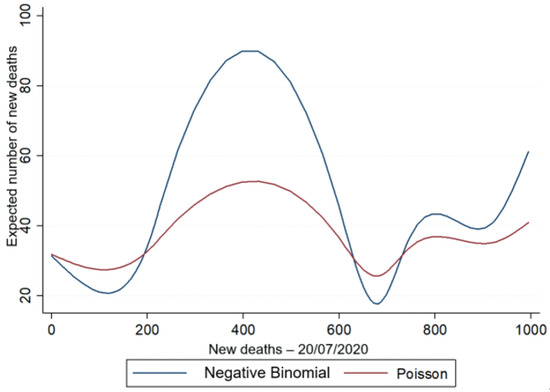
Figure 5. Predicted amount vs. the actual occurrence of new deaths for the NB2 and Poisson models with the explanatory variable age.

Figure 4 and Figure 5 show that the variable of the predicted amount of new daily deaths is higher for the negative binomial regression model, in which the estimation can capture the existence of overdispersion in the data as a result of the variable (σ² = 9.753) of new deaths, presented in Table 4, thus proving the best fit of the negative binomial regression model in relation to the Poisson model.

4.4. Zero-Inflated Negative Binomial Type Model Estimation

Considering the daily occurrence of new deaths from COVID-19 after the application of the first dose of the COVID-19 vaccine (20 July 2022), Table 9 and Table 10, respectively, present the results of the estimates of the ZINB regression models, with the HDI (Table 9) and age (Table 10). It is sought to analyse simultaneously whether the probability of non-occurrence of new deaths (occurrence of structural zeros) and whether the event of a given count is influenced by the HDI/age.

Table 9. Regression 3 results: new deaths before the application of the first dose of vaccine explained by HDI.

Likelihood-ratio test (χ2)			−293.104
Probabilities (χ2)			6.68
Likelihood-ratio test (χ2)			0.0097
Variable	Coefficient	Standard Error	z	p	Confidence Interval 95%
Daily number of new deaths
Constant	−3.443	2.343	−1.47	0.142	−8.035	1.150
IDH	7.405	2.799	2.65	0.008	1.919	12.8905
Inflation
Constant	9.820	3.896	2.52	0.012	2.184	17.456
IDH	−14.098	6.095	−2.31	0.021	−26.044	−2.152
Variable new daily deaths	7.004	2.188			3.797	12.919
Likelihood-ratio test (χ2)	3320.68			0.000

Table 10. Regression 4 results: new deaths before application of the first dose of vaccine explained by age.

Likelihood-ratio test (χ2)			−293.3356
Probability (χ2)			6.45
Likelihood-ratio test (χ2)			0.0111
Variable	Coefficient	Standard Error	z	p	Confidence Interval 95%
Daily number of new deaths
Constant	−10.858	5.102	−2.13	0.033	−20.858	−0.858
Age	0.173	0.066	0.066	0.008	0.045	0.302
Inflation
Constant	25.954	11.007	2.36	0.018	4.381	47.526
Age	−0.366	0.158	−2.31	0.021	−0.676	−0.055
Variable new daily deaths	7.684	1.944			4.680	12.617
Likelihood-ratio test (χ2)	3214.61			0.000

Table 9 and Table 10 include the probability of not-occurring new daily deaths (occurrence of structural zeros, binary distribution) and the occurrence of a specific death count after the application of the first dose of vaccine, which is explained by HDI and age.

The estimated parameters of the HDI and age are statistically different from zero, to 95% confidence level, to explain the behaviour of the daily number of new deaths and the excessive number of zeros in the dependent variable, of new deaths. The result of the likelihood-ratio test (likelihood-ratio test, χ² = 3320.68; p = 0.00, χ² = 3214.61; p = 0.00) for the parameter of the variable of the independent variable (with an estimated value equal to 7.004 and 7.684) that allows comparing the adequacy of the negative binomial model concerning the Poisson model, is statistically significant, at the level of 5% and the confidence interval at 95% of this parameter does not contain zero, which proves the existence of overdispersion in the data. Thus, the expected average amount of new daily deaths after the application of the first dose of vaccine is 51.839 and 1.766 × 10⁻¹⁶; however, considering the regional average values of the HDI and age of the WHO member countries grouped into six regions, the predicted average of new deaths is presented in Table 11.

Table 11. Expected average number of new daily deaths per region.

Region (WHO)	Average HDI	Expected Average of New Daily Deaths	Average Age	Expected Average of New Daily Deaths
AFRO	0.550	0.209	63.278	0.063
AMRO	0.758	6.196	75.352	7.458
EMRO	0.700	2.913	73.3519	4.472
EURO	0.859	16.786	78.376	14.168
SEARO	0.674	1.977	72.621	3.615
WPRO	0.744	5.235	74.092	5.463

Table 11 shows that regions with lower HDI and age have lower daily occurrences of new deaths. Thus, the expected average number of new daily deaths per region, explained by HDI and age, ranges from 0.209 to 0.063 (AFRO) and 16.786 to 14.168 (EURO).

Table 12 and Figure 6, considering the HDI explanatory variable, illustrate the behaviour of observed and estimated probability distributions of occurrence from zero to nine new daily deaths after the application of the first dose of vaccine, obtained by the ZIP regression models and ZINB.

Table 12. Comparison of observed and estimated probabilities for each count of new deaths and their terms of error for zip and zinb models.

Score	Panel A—Explanatory Variable HDI							Panel B—Explanatory Variable Age
	Poisson Model ZIP				Negative binomial Model ZINB			Poisson Model ZIP			Negative Binomial Model ZINB
	Probability		Difference	Pearson Value	Prob Est	Difference	Pearson Value	Prob Est	Difference	Pearson Value	Prob Est	Difference	Pearson Value
	Observed	Death
0	0.734	0.734	0.000	0.000	0.734	0.001	0.000	0.734	0.000	0.000	0.733	0.001	0.000
1	0.016	0.001	0.014	26.341	0.042	0.026	3.027	0.002	0.014	19.610	0.043	0.027	3.267
2	0.032	0.002	0.03	69.991	0.024	0.008	0.554	0.003	0.029	63.378	0.024	0.008	0.470
3	0.021	0.003	0.018	21.896	0.017	0.005	0.251	0.003	0.018	21.721	0.017	0.004	0.216
4	0.021	0.003	0.018	19.538	0.013	0.008	1.05	0.003	0.018	20.171	0.013	0.008	0.992
5	0.021	0.003	0.018	18.96	0.01	0.011	2.106	0.003	0.018	19.346	0.011	0.011	2.040
6	0.011	0.003	0.007	3.201	0.009	0.002	0.07	0.003	0.007	3.066	0.009	0.002	0.064
7	0.011	0.003	0.007	3.174	0.008	0.003	0.223	0.003	0.007	2.756	0.008	0.003	0.215
8	0.005	0.003	0.002	0.223	0.007	0.001	0.054	0.004	0.002	0.124	0.007	0.001	0.056
9	0.005	0.004	0.002	0.172	0.006	0.001	0.014	0.004	0.001	0.074	0.006	0.001	0.015
Total	0.878	0.760	0.117	163.496	0.868	0.066	7.349	0.762	0.115	150.247	0.870	0.067	7.337
Max difference	0.030				0.012			0.029			0.012
Difference average	−0.026				0.007			−0.027			0.007

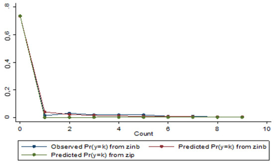
Figure 6. Distribution of observed and predicted probabilities of occurrence of new deaths for the ZINB and ZIP models with the HDI explanatory variable.

It is the contact that the ZINB model presents a better fit to the observed distribution than the estimated probability distribution of the ZIP model. The maximum difference between observed and estimated probabilities is greater for ZIP models (0.030 and 0.029) than for the ZINB model (0.012). Similarly, the averages of these differences in module (from 0.026 to 0.007 for ZINB) and Pearson total value (from 163.4960 to 7.349 for ZINB, panel A; from 163.4960 to 7.349 for ZINB, panel B) are higher for ZIP models.

Changes in the relationship between the HDI and COVID-19 mortality over time may be explained by differences in vaccination coverage, demographic exposure, viral variants, public health responses, and reporting heterogeneity across countries.

4.5. Variance Analysis—Variance Decomposition Through Multilevel Modelling

This section presents the empirical results obtained from the statistical models described in the Research Methodology section.

From Table 13, estimates of two-level multilevel regression models (Level 1, time and Level 2, country) are presented with repeated measures for an unbalanced panel data structure of the 185 WHO member countries, with daily observations (12 January 2020 to 20 July 2022) ranging from 108 (Samoa) to 921 (China), totalling 147,879.

Table 13. Variance decomposition—null model.

	Panel A Dependent Variable—Accumulated Cases of Infection			Panel B Dependent Variable—Accumulated Deaths
Fixed Effect	Coefficient	Standard Error	z	Coefficient	Standard Error	z
Global average	10.938 ***	0.147	74.28	6.706 ***	0.171	39.20
Random effect	Variance component	Standard Error	z	Variance component	Standard Error	z
Level 1 (time)
Temporal variation (rti)	3.849 ***	0.014	271.75	3.143 ***	0.012	271.75
Level 2 (country)
Country Variation—Intercept (u0i)	4.006 ***	0.418	9.58	5.409 ***	0.565	9.58
Variance decomposition	% per level			% per level
Level 1 (time)	49,002			36,756
Level 2 (country)	50,998			63,244
LR test vs. OLS	100,000 ***			140,000 ***
Log restricted-likelihood	−310,110.06			−295,179.76

Note: *** p < 1%.

Thus, Table 13 presents the results of the decomposition of variance estimated from a null model, represented by the Equation (4). Panels A and B, respectively, show the decomposition of the variance between levels with infection and accumulated death by COVID-19 as a dependent variable. It is observed that there is variability in the accumulated amounts of occurrences of infection and death by COVID-19 over time under analysis (12 January 2020 to 20 July 2022) and that there is variability in the cumulative amounts of COVID-19 infection and death occurrences over time between different countries.

The result of the likelihood-ratio test (LR = 100,000; p. χ² = 0.00 < 0.01) indicates that at the significance level of 5%, the random effect intercepts are not equal to zero, thus suggesting that for the data of this study and the period under analysis, the estimation of a linear regression model by OLS is not the most indicated. The decomposition of the variance holds that 49.002% (z = 271, 75; p < 0.01; panel A) and 36.756% (z = 271.75; p < 0.01; panel B) of variability, respectively, in the occurrences of infection and death by COVID-19 is explained by the temporal evolution in each country, but 50.998% (z = 9.58; p < 0.01; panel A) and 63.244% (z = 9.58; p < 0.01; panel B) of the total variable in occurrences is due to differences between countries, that is, the variability in the accumulated amounts of infection and death by COVID-19 is more significant among countries, considering the period under analysis.

Table 14 presents the results of estimating a linear trend model with random intercepts and slopes that include the trend at level 1 (time), represented by the Equation (11). Statistical significance was observed at the level of 5% of the parameters of fixed effects and the variable (σ² = 0.871; z = 271.57; p < 0.01; τ₀₀ = 3.966 z = 9.58; p < 0.01; τ₁₁ = 5.57 × 10⁻⁶; z = 9.35; p < 0.05; panel A; σ² = 0.864; z = 271.57; p < 0.01; τ₀₀ = 5.306; z = 9.58; p < 0.01; τ₁₁ = 6.33 × 10⁻⁶; z = 9.31; p < 0.01; panel B). The linear trend variable with fixed effects, DAY, is positive, suggesting that the other constant conditions, occurrences of infection and death by COVID-19 each day, increased on average 100.702% (and (0.007) infection, panel A) and 100.602% (and (0.006) death, panel B).

Table 14. Variance decomposition—linear trend model with random effects of intercepts and slopes.

	Panel A Dependent Variable—Accumulated Cases of Infection			Panel B Dependent Variable—Accumulated Deaths
Fixed Effect	Coefficient	Standard Error	z	Coefficient	Standard Error	z
Global average	8.193 ***	0.146	55.93	4.311 ***	0.169	25.44
DAY	0.007 ***	1.75 × 10−4	39.35	0.006 ***	1.86 × 10−4	32.82
Random effect	Variance component	Standard Error	z	Variance component	Standard Error	z
Level 1 (time)
Temporal variation (rti)	0.871 ***	0.003	271.57	0.864 ***	0.003	271.57
Level 2 (country)
Country variation—Intercept (u0i)	3.966 ***	0.414	9.58	5.306 ***	0.554	9.58
Country variation—slope (u1i)	5.57 × 10−6 ***	5.96 × 10−7	9.35	6.33 × 10−6 ***	6.8 × 10−7	9.31
Variance decomposition	% per level			% per level
Level 1 (time)	18.007			14.00
Level 2 (country)	81.993			86.00
LR test vs. OLS	250,000 ***			280,000 ***
Log restricted-likelihood	−200,884.06			−200,312.36
LR test—random intercepts model vs. model with random intercepts and slopes		38,921.02 ***			41,292.12 ***

Note: *** p < 1%.

As expected, the result of the likelihood-ratio test (LR = 250,000; p. χ² = 0.00 < 0.01; panel A; LR = 280,000; p. χ² = 0.00 < 0.01; panel B) at the significance level of 5%, indicates that the intercepts and random slopes are not equal to zero, so the estimation of a linear adjustment model by OLS is discarded. In addition, the likelihood-ratio test was designed to compare the performances in the estimates of linear trend models with random intercepts and slopes. (LR = 38,921.02; p. χ² = 0.00 < 0.01; panel A; LR = 41,292.12; p. χ² = 0.00 < 0.01; panel B) maintains that the linear trend model with random effects of intercepts and slopes (represented by Equation (11)) is the most appropriate. In this context, the decomposition of the variance given by the correlation between the natural logarithms of the occurrences of infection (panel A) and death (panel B) indicates that the random effects of infection and deaths between different countries represent more than 81% (panel A) and 85% (panel B) of the total variance.

In this sequence, Table 15 presents the results of the final complete model, of the linear trend with random effects of intercepts and slopes and the variable of level 2 (country), the HDI, considering the dependent variable accumulated amount of daily infection by COVID-19 (panel A) and accumulated amount of daily death by COVID-19 (panel B).

Table 15. Variance decomposition—linear trend model with random effects of intercepts and slopes— First variable set.

	Panel A Dependent Variable—Accumulated Cases of Infection			Panel B Dependent Variable—Accumulated Deaths
Fixed Effect	Coefficient	Standard Error	z	Coefficient	Standard Error	z
Global Average	5.469 ***	0.693	7.90	1.119	0.800	1.40
DAY	0.003 ***	0.001	3.80	0.006 ***	1.86 × 10−4	32.82
IDH	3.774 ***	0.939	4.02	4.422 ***	1.085	4.07
HDIDAY	0.005 ***	0.001	4.85
Random effect	Variance component	Standard Error	z	Variance component	Standard Error	z
Level 1 (time)
Temporal variable (rti)	0.871 ***	0.003	271.58	0.864 ***	0.003	271.57
Level 2 (country)
Country variation—Intercept (u0i)	3.662 ***	0.383	9.55	4.891 ***	0.512	9.56
Country variation—slope (u1i)	4.91 × 10−6 ***	5.31 × 10−7	9.25	6.33 × 10−6 ***	6.8 × 10−7	9.31
Variable decomposition	% per level			% per level
Level 1 (tempo)	19.212			15.010
Level 2 (country)	80.788			84.990
LR test vs. OLS	220,000 ***			260,000 ***
Log restricted-likelihood	−200,870.25			−200,303.38

Note: *** p < 1%.

The multilevel variance decomposition indicates that a substantial proportion of the total variability in COVID-19 infection and mortality is attributable to between-country differences, reinforcing the importance of structural and contextual factors beyond short-term temporal fluctuations.

Through the analysis of Table 15, it is observed that the parameters of fixed effects and the components of variables (σ² = 0.871; z = 271.58; p < 0.01; τ₀₀ = 3.662; z = 9.55; p < 0.01; τ₁₁ = 4.91 × 10⁻⁶; z = 9.25; p < 0.05; panel A; σ² = 0.864; z = 271.57; p < 0.01; τ₀₀ = 4.891; z = 9.56; p < 0.01; τ11 = 6.33 × 10⁻⁶; z = 9.31; p < 0.01; panel B) are positive and statistically significant, at the significance level of 5%, to explain the differences in the occurrences of infection and death by COVID-19 in a given country. Keeping the other conditions contained, it is observed that, on average, the HDI contributes to the increase in occurrences of infection and death by COVID-19 in a given country, in 43.554 (e^(3.774)) infections, panel A, and 83.263 (e^(4.422)) deaths, panel B, per day. The decomposition of the variance between levels indicates that 80.788% (z = 49.70; p < 0.01; panel A) and 84.99% (z = 63.63, p < 0.01; panel B) are due to differences in infection and death between countries. As expected, the likelihood-ratio test result (LR = 188.51, p. χ² = 0.00 < 0.01) against (LR = 260,000, p. χ² = 0.00 < 0.01) indicates statistical significance at the level of 5%, attesting that the intercepts and slopes of random effects are in fact different from zero, so the estimation of a regression model by OLS is discarded in favour of multilevel regression modelling.

In this case, Figure 7 states that the multilevel regression model presents a better linear fit than the OLS model.

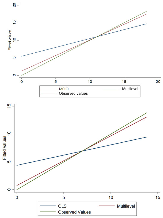
Figure 7. Predicted values by OLS and multilevel vs. observed values of the accumulated amount of daily deaths by COVID-19.

Figure 8 and Figure 9, respectively, enable the visualisation of random intercepts and slopes of 20 of the 185 WHO member countries/states that presented the first ten and the last ten random residues.

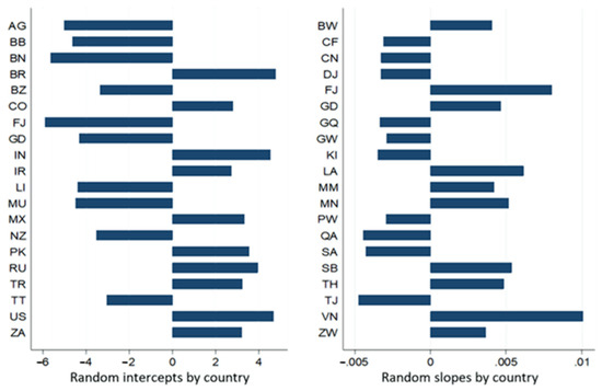
Figure 8. Expected values of intercepts and slopes of random effects per country estimated by the final complete model of the dependent variable accumulated amount of infection.

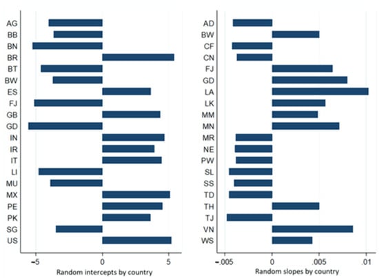
Figure 9. Expected values of intercepts and slopes of random effects per country estimated by the final complete model of the dependent variable accumulated amount of deaths.

The rates of expected variations in intercepts and slopes, respectively, of the natural logarithm of accumulated amounts of infection and death ranged from 0.003 (e^−5.908; Fiji, high HDI) to 119,909 (e^4.787; Brazil, HDI, high); from 0.995 (e^−0.005; Tajikistan, Mediun IHD) to 1.01 (e^0.010; Vietnam, Mediun HDI) to 0.004 (e^−5.582; Grenada, HDI, high) to 224,337 (e^5.413, Brazil, high HDI); and from 0.995 (e^−0.005; Tajikistan, Mediun IHD) to 1.01 (e^0.010; Laos, high HDI).

The results presented in Table 15 show that the natural logarithm of accumulated amounts of infection and death from the 185 WHO member countries followed a linear trend over time, and there were significant differences in intercepts and slopes between the different countries. The HDI explains part of this variability.

Table A1 and Table A2, and Table A3, respectively, in Appendix A, Appendix B and Appendix C, show the results of the final complete models, with random effects of the intercepts, slopes, and level 2 variable (country), represented by the three basic dimensions of the HDI, i.e., age, education, and GNI. In this sequence, a positive and statistically significant relationship is observed, at the significance level of 5%, between the three basic dimensions of the HDI and the accumulated occurrences of infection and death by COVID-19. Keeping the other constant conditions, on average, age, option and income, respectively, increased the circumstances of infection and death by COVID-19 per day in a given country by 1.077 (e^0.074); 1,168 (e^0.155) and 1 (e^0.0000184), considering the amount of infection (panel A) and 1.092 (e^0.088); 1.197 (e^0.18) and 1 (e^0.0000213) are the death amount (panel B). The random effects of infection and death by COVID-19 among the various countries under analysis make up between 80.99% (Table 15, infection explained by age) and 81.491% (Table A2, infection explained by GNI) and between 85.038% (Table 15, death explained by age) and 85.592% (Table A2, death explained by GNI) of the total variable of the residues.

4.6. Hypotheses Assessment

The empirical findings allow a direct reassessment of the hypotheses formulated in the Introduction. Hypothesis H1, which proposed a statistically significant association between the HDI and COVID-19 mortality across the WHO member states, is supported by the negative binomial and multilevel regression results, particularly in the pre-vaccination period, where the HDI showed a positive and statistically significant relationship with mortality rates. Hypothesis H2, stating that the population age structure is positively associated with COVID-19 mortality, is likewise confirmed, as age consistently exhibited statistically significant positive coefficients in both count and zero-inflated models. Finally, Hypothesis H3, which suggested that the relationship between the HDI and COVID-19 mortality varies across countries and over time, is also supported by the multilevel variance decomposition results, which revealed substantial between-country variability and statistically significant random effects in intercepts and slopes. Together, these findings reinforce the robustness of the proposed hypotheses within the structured longitudinal modelling framework adopted in this study.

4.7. Limitations

A key limitation of this study is the use of absolute death counts without explicit population offsets, which may limit cross-country comparability. Therefore, the estimated coefficients should be interpreted as conditional statistical associations rather than standardised mortality risks.

5. Conclusions

The originality of this study does not reside in identifying new determinants of COVID-19 mortality, but in the methodological integration of count data regression and multilevel longitudinal modelling, providing a comprehensive analytical framework applicable to large-scale epidemiological datasets.

Several studies have applied different techniques to evaluate the relationship between the occurrences of infection and death by COVID-19, the HDI, and basic components of human development for a given temporal exposure. This research followed the pioneering studies of [6,40], but the counting data differed by sample, temporal exposure, and modelling. Moreover, considering that the COVID-19 pandemic has manifested differently in each country, research has evolved into a long-term perspective.

Thus, initially, from two samples, this study sought to evaluate the relationship between the occurrence of new daily deaths by COVID-19 and the HDI and age of the 188 WHO member countries for daily temporal exposure, respectively, on 20 July 2020, before the application of the first dose of the vaccine, and 20 July 2022, the date after the application of at least one dose of the vaccine in a WHO country/member state.

Based on the results of the tests of [55,56], the NB2 regression modelling was applied, considering the occurrence of new deaths on 20 July 2020 and ZINB regression modelling for the data of 20 July 2022. The estimates maintain that the daily occurrence rate of new deaths before the application of the first vaccine dose, explained by the HDI and age, respectively, was on average multiplied by a factor of 1290.797 (HDI, 128,979.7% higher) and 1.145 (age, 14.5% higher). However, after the application of the first dose of the vaccine, the probability of not-occurring new daily deaths explained by the HDI and age was, on average, 51.839 (HDI) and 1.766 × 10⁻¹⁶ (age). On the other hand, the average expected number of new daily deaths per region, according to the WHO classification, ranged from 0.209 (HDI, AFRO) to 16.786 (HDI, EURO) to 0.063 (AFRO age) and 14.168 (age, EURO).

Secondly, from a panel data sample with repeated measurements from the 185 WHO member countries/states with daily observations from 12 January 2020 to 20 July 2022, we sought to assess through multilevel regression modelling with two levels (time and country/state) whether the accumulated amounts of infection and death, between the different countries, followed a linear trend over time, if there were significant variables of intercepts and slopes between the different countries, and if the HDI and the three essential components of human development explain part of this variability. Based on the estimation of a non-conditional model, it was possible to attest to the existence of variability in the amounts of occurrences of infection and death over the period analysed, over time, and between the different countries/states. 50.998% and 63.244% of the total variability are due to differences between countries/states. The linear trend model maintains that there is a temporal variation of random effects of intercepts and slopes in the amounts of occurrences of infection and death, respectively, in which 81.993% and 86% of this variation is due to differences between countries. The HDI explains 80.788% and 84.99% of the total variability in the occurrences of infection and death, respectively. In addition, decomposing the HDI revealed that, respectively, age, education, and GNI explain 80.899%, 81.163% and 81.491% of the total variability of the amount of infection, and 85.038%, 85.322% and 85.592% of the total variability of the amount of death among the 185 countries/states.

The results of this study show that social isolation measures and the vaccination campaign against COVID-19 contributed to the reduction in new deaths worldwide.

For a given exposure, even if the same sample is maintained, the regression models for counting data change distribution. The definition of a non-daily temporal exposure (reflected in this study) for future research offers a new perspective on the relationship between the occurrence of death and the HDI. On the other hand, although the HDI and income size are risk factors for death by, several studies [35,36,39,59,60,61,62,63] attest that regions with a low HDI and income also present greater vulnerability to the pandemic of COVID-19, because of this evidence and, considering that the HDI implies only health, education and income, an index that reflects inequalities and poverty applied in a multilevel study, which includes data from mesoregions may present new results that complement the impact of human development on the COVID-19 pandemic.

This study contributes methodologically by demonstrating how integrated count and multilevel modelling can be applied to large-scale epidemiological data. Substantively, it highlights the role of structural and demographic heterogeneity in shaping COVID-19 mortality patterns. These insights are relevant for both theoretical research and evidence-informed public health decision-making.

References

- UDNP Gender Inequality and the COVID-19 Crisis: A Human Development Perspective. 2020. Available online: https://hdr.undp.org/content/gender-inequality-and-covid-19-crisis-human-development-perspective (accessed on 20 January 2023).
- Samudra, A.; Samudra, A. Understanding Relationship between Human Development Index and COVID Infection Rate-A Study of Districts in Maharashtra. Shodh Sarita Multidiscip. J. Forthcom. 2020. [Google Scholar] [CrossRef]
- Fauci, A.S.; Lane, H.C.; Redfield, R.R. COVID-19—Navigating the uncharted. N. Engl. J. Med. 2020, 382, 1268–1269. [Google Scholar] [CrossRef]
- Russo, F.P. COVID-19 in Padua, Italy: Not just an economic and health issue. Nat. Med. 2020, 26, 806. [Google Scholar] [CrossRef] [PubMed]
- Hui, D.S.C.; Zumla, A. Severe acute respiratory syndrome: Historical, epidemiologic, and clinical features. Infect. Dis. Clin. 2019, 33, 869–889. [Google Scholar]
- Liu, A. Philanthropy and humanity in the face of a pandemic—A letter to the editor on “World Health Organization declares global emergency: A review of the 2019 novel coronavirus (COVID-19)” (Int J surg 2020; 76: 71–6). Int. J. Surg. 2020, 79, 10. [Google Scholar] [CrossRef]
- Andrea, R.; Giuseppe, R. COVID-19 and Italy: What next? Lancet 2020, 395, 1225–1228. [Google Scholar] [CrossRef]
- Essien, U.R.; Eneanya, N.D.; Crews, D.C. Prioritizing equity in a time of scarcity: The COVID-19 pandemic. J. Gen. Intern. Med. 2020, 35, 2760–2762. [Google Scholar] [CrossRef]
- Fallucchi, F.; Faravelli, M.; Quercia, S. Fair allocation of scarce medical resources in the time of COVID-19: What do people think? J. Med. Ethics 2021, 47, 3–6. [Google Scholar] [CrossRef]
- Taylor, L. Covid-19: Is Manaus the final nail in the coffin for natural herd immunity? BMJ 2021, 372, n394. [Google Scholar] [CrossRef]
- Thazhathedath Hariharan, H.; Surendran, A.T.; Haridasan, R.K.; Venkitaraman, S.; Robert, D.; Narayanan, S.P.; Mammen, P.C.; Siddharth, S.R.; Kuriakose, S.L. Global COVID-19 transmission and mortality—Influence of human development, climate, and climate variability on early phase of the pandemic. GeoHealth 2021, 5, e2020GH000378. [Google Scholar] [CrossRef]
- Zeiser, F.A.; Donida, B.; da Costa, C.A.; de Oliveira Ramos, G.; Scherer, J.N.; Barcellos, N.T.; Alegretti, A.P.; Ikeda, M.L.R.; Müller, A.P.W.C.; Bohn, H.C. First and second COVID-19 waves in Brazil: A cross-sectional study of patients’ characteristics related to hospitalization and in-hospital mortality. Lancet Reg. Health-Am. 2022, 6, 100107. [Google Scholar] [CrossRef]
- Ahmed, F.; Ahmed, N.; Pissarides, C.; Stiglitz, J. Why inequality could spread COVID-19. Lancet Public Health 2020, 5, e240. [Google Scholar] [CrossRef]
- Dyer, O. Trump claims public health warnings on COVID-19 are a conspiracy against him. BMJ 2020, 368, m941. [Google Scholar] [CrossRef]
- Gozzi, N.; Tizzoni, M.; Chinazzi, M.; Ferres, L.; Vespignani, A.; Perra, N. Estimating the effect of social inequalities on the mitigation of COVID-19 across communities in Santiago de Chile. Nat. Commun. 2021, 12, 1–9. [Google Scholar] [CrossRef]
- Liu, J.H. Majority world successes and European and American failure to contain COVID-19: Cultural collectivism and global leadership. Asian J. Soc. Psychol. 2021, 24, 23–29. [Google Scholar] [CrossRef] [PubMed]
- Marson, F.A.L.; Ortega, M.M. COVID-19 in Brazil. Pulmonology 2020, 26, 241. [Google Scholar] [CrossRef]
- Peres, I.T.; Bastos, L.; Gelli, J.G.M.; Marchesi, J.F.; Dantas, L.F.; Antunes, B.B.P.; Maçaira, P.M.; Baião, F.A.; Hamacher, S.; Bozza, F.A. Sociodemographic factors associated with COVID-19 in-hospital mortality in Brazil. Public Health 2021, 192, 15–20. [Google Scholar] [CrossRef] [PubMed]
- Souza, R.D.F.; Fávero, L.P.; Haddad, M.F.C.; Corrêa, H.L. Multilevel evidence on how policymakers may reduce avoidable deaths due to COVID-19: The case of Brazil. Int. J. Math. Oper. Res. 2022, 21, 321–337. [Google Scholar] [CrossRef]
- Aggarwal, A.; Shrivastava, A.; Kumar, A.; Ali, A. Clinical and epidemiological features of SARS-CoV-2 patients in SARI ward of a tertiary care centre in New Delhi. J. Assoc. Physicians India 2020, 68, 19–26. [Google Scholar] [PubMed]
- Chen, N.; Zhou, M.; Dong, X.; Qu, J.; Gong, F.; Han, Y.; Qiu, Y.; Wang, J.; Liu, Y.; Wei, Y.; et al. Epidemiological and Clinical Characteristics of 99 Cases of 2019 4 Novel Coronavirus Pneumonia in Wuhan, China: A Descriptive Study. Lancet 2020, 395, 5. [Google Scholar] [CrossRef] [PubMed]
- Grasselli, G.; Zangrillo, A.; Zanella, A.; Antonelli, M.; Cabrini, L.; Castelli, A.; Cereda, D.; Coluccello, A.; Foti, G.; Fumagalli, R. Baseline characteristics and outcomes of 1591 patients infected with SARS-CoV-2 admitted to ICUs of the Lombardy Region, Italy. JAMA 2020, 323, 1574–1581. [Google Scholar] [CrossRef]
- Guzik, T.J.; Mohiddin, S.A.; Dimarco, A.; Patel, V.; Savvatis, K.; Marelli-Berg, F.M.; Madhur, M.S.; Tomaszewski, M.; Maffia, P.; D’acquisto, F. COVID-19 and the cardiovascular system: Implications for risk assessment, diagnosis, and treatment options. Cardiovasc. Res. 2020, 116, 1666–1687. [Google Scholar] [CrossRef]
- Jiang, F.; Deng, L.; Zhang, L.; Cai, Y.; Cheung, C.W.; Xia, Z. Review of the clinical characteristics of coronavirus disease 2019 (COVID-19). J. Gen. Intern. Med. 2020, 35, 1545–1549. [Google Scholar] [CrossRef]
- Karami, M.; Mirzaei, M.; Shahbazi, F.; Keramat, F.; Jalili, E.; Bashirian, S.; Heidarimoghadam, R.; Bathaei, J.; Khazaei, S. Predictors of death in patients with COVID-19: A cross-sectional study in West of Iran. Med. J. Islam. Repub. Iran 2021, 35, 103. [Google Scholar] [CrossRef] [PubMed]
- Khan, M.; Khan, H.; Khan, S.; Nawaz, M. Epidemiological and clinical characteristics of coronavirus disease (COVID-19) cases at a screening clinic during the early outbreak period: A single-centre study. J. Med. Microbiol. 2020, 69, 1114. [Google Scholar] [CrossRef] [PubMed]
- Li, H.; Wang, S.; Zhong, F.; Bao, W.; Li, Y.; Liu, L.; Wang, H.; He, Y. Age-dependent risks of incidence and mortality of COVID-19 in Hubei Province and other parts of China. Front. Med. 2020, 7, 190. [Google Scholar] [CrossRef]
- Nicotra, E.F.; Pili, R.; Gaviano, L.; Carrogu Gpietro Berti, R.; Grassi, P.; Petretto, D.R. COVID-19 and the excess of mortality in Italy from January to April 2020: What are the risks for oldest old? J. Public Health Res. 2022, 11, jphr-2021. [Google Scholar] [CrossRef]
- Ramos-Rincon, J.-M.; Buonaiuto, V.; Ricci, M.; Martín-Carmona, J.; Paredes-Ruíz, D.; Calderón-Moreno, M.; Rubio-Rivas, M.; Beato-Pérez, J.-L.; Arnalich-Fernández, F.; Monge-Monge, D. Clinical characteristics and risk factors for mortality in very old patients hospitalized with COVID-19 in Spain. J. Gerontol. Ser. A 2021, 76, e28–e37. [Google Scholar] [CrossRef]
- Sansone, N.M.S.; Boschiero, M.N.; Marson, F.A.L. Epidemiologic Profile of Severe Acute Respiratory Infection in Brazil During the COVID-19 Pandemic: An Epidemiological Study. Front. Microbiol. 2022, 13, 911036. [Google Scholar] [CrossRef] [PubMed]
- Suleyman, G.; Fadel, R.A.; Malette, K.M.; Hammond, C.; Abdulla, H.; Entz, A.; Demertzis, Z.; Hanna, Z.; Failla, A.; Dagher, C. Clinical characteristics and morbidity associated with coronavirus disease 2019 in a series of patients in metropolitan Detroit. JAMA Netw. Open 2020, 3, e2012270. [Google Scholar] [CrossRef]
- Wang, W.; Tang, J.; Wei, F. Updated understanding of the outbreak of 2019 novel coronavirus (2019-nCoV) in Wuhan, China. J. Med. Virol. 2020, 92, 441–447. [Google Scholar] [CrossRef]
- Xiong, S.; Liu, L.; Lin, F.; Shi, J.; Han, L.; Liu, H.; He, L.; Jiang, Q.; Wang, Z.; Fu, W. Clinical characteristics of 116 hospitalized patients with COVID-19 in Wuhan, China: A single-centered, retrospective, observational study. BMC Infect. Dis. 2020, 20, 1–11. [Google Scholar] [CrossRef]
- Zhou, L.; Puthenkalam, J.J. Effects of the Human Development Index on COVID-19 Mortality Rates in High-Income Countries. Eur. J. Dev. Stud. 2022, 2, 26–31. [Google Scholar] [CrossRef]
- Alberti, A.; da Silva, B.B.; de Jesus, J.A.; Zanoni, E.M.; Grigollo, L.R. Associação do maior número de mortes por COVID-19 e o Índice de Desenvolvimento Humano (IDH) de Cidades Catarinenses/Association of the highest number of deaths by COVID-19 and the Human Development Index (HDI) of cities in Santa Catarina. ID Online Rev. Psicol. 2021, 15, 427–434. [Google Scholar] [CrossRef]
- Baggio, J.A.O.; Machado, M.F.; do Carmo, R.F.; da Costa Armstrong, A.; dos Santos, A.D.; de Souza, C.D.F. COVID-19 in Brazil: Spatial risk, social vulnerability, human development, clinical manifestations and predictors of mortality–a retrospective study with data from 59 695 individuals. Epidemiol. Infect. 2021, 149, e100. [Google Scholar] [CrossRef]
- Buheji, M.; AlDerazi, A.; Ahmed, D.; Bragazzi, N.L.; Jahrami, H.; Hamadeh, R.R.; BaHammam, A.S. The association between the initial outcomes of COVID-19 and the human development index: An ecological study. Hum. Syst. Manag. 2022, 41, 303–313. [Google Scholar] [CrossRef]
- Neto, D.M.F.; Morbeck, N.B.M.; Welter, Á.; Panontin, J.F. Relação entre índice de desenvolvimento humano e número de casos de Covid-19 em cidades do tocantins. Singul. Saúde Biológicas 2021, 1, 23–27. [Google Scholar]
- Palamim, C.V.C.; Boschiero, M.N.; Valencise, F.E.; Marson, F.A.L. Human Development Index Is Associated with COVID-19 Case Fatality Rate in Brazil: An Ecological Study. Int. J. Environ. Res. Public Health 2022, 19, 5306. [Google Scholar] [CrossRef]
- Shahbazi, F.; Khazaei, S. Socio-economic inequality in global incidence and mortality rates from coronavirus disease 2019: An ecological study. New Microbes New Infect. 2020, 38, 100762. [Google Scholar] [CrossRef]
- Troumbis, A.Y. Testing the socio-economic determinants of COVID-19 pandemic hypothesis with aggregated Human Development Index. J. Epidemiol. Community Health 2021, 75, 414–415. [Google Scholar] [CrossRef]
- Upadhyay, A.K.; Shukla, S. Correlation study to identify the factors affecting COVID-19 case fatality rates in India. Diabetes Metab. Syndr. Clin. Res. Rev. 2021, 15, 993–999. [Google Scholar] [CrossRef]
- Bermudi, P.M.M.; Lorenz, C.; de Aguiar, B.S.; Failla, M.A.; Barrozo, L.V.; Chiaravalloti-Neto, F. Spatiotemporal ecological study of COVID-19 mortality in the city of São Paulo, Brazil: Shifting of the high mortality risk from areas with the best to those with the worst socio-economic conditions. Travel Med. Infect. Dis. 2021, 39, 101945. [Google Scholar] [CrossRef] [PubMed]
- Bonanad, C.; García-Blas, S.; Tarazona-Santabalbina, F.; Sanchis, J.; Bertomeu-González, V.; Facila, L.; Ariza, A.; Nunez, J.; Cordero, A. The effect of age on mortality in patients with COVID-19: A meta-analysis with 611,583 subjects. J. Am. Med. Dir. Assoc. 2020, 21, 915–918. [Google Scholar] [CrossRef]
- Maciel, J.A.C.; Castro-Silva, I.I.; de Farias, M.R. Initial analysis of the spatial correlation between the incidence of COVID-19 and human development in the municipalities of the state of Ceará in Brazil. Rev. Bras. Epidemiol. 2020, 23, e200057. [Google Scholar] [CrossRef]
- Mirahmadizadeh, A.; Ghelichi-Ghojogh, M.; Vali, M.; Jokari, K.; Ghaem, H.; Hemmati, A.; Jafari, F.; Dehghani, S.S.; Hassani, A.H.; Jafari, A. Correlation between human development index and its components with COVID-19 indices: A global level ecologic study. BMC Public Health 2022, 22, 1–8. [Google Scholar] [CrossRef]
- Papadopoulos, V.P.; Emmanouilidou, A.; Yerou, M.; Panagaris, S.; Souleiman, C.; Varela, D.; Avramidou, P.; Melissopoulou, E.; Pappas, C.; Iliadou, Z. SARS-CoV-2 Vaccination Coverage and Key Public Health Indicators May Explain Disparities in COVID-19 Country-Specific Case Fatality Rate Within European Economic Area. Cureus 2022, 14, e22989. [Google Scholar] [CrossRef] [PubMed]
- Ribeiro, K.B.; Ribeiro, A.F.; Veras MAde, S.M.; de Castro, M.C. Social inequalities and COVID-19 mortality in the city of São Paulo, Brazil. Int. J. Epidemiol. 2021, 50, 732–742. [Google Scholar] [CrossRef]
- Varkey, R.S.; Joy, J.; Sarmah, G.; Panda, P.K. Socio-economic determinants of COVID-19 in Asian countries: An empirical analysis. J. Public Aff. 2021, 21, e2532. [Google Scholar] [CrossRef] [PubMed]
- Choi, K.W.; Chau, T.N.; Tsang, O.; Tso, E.; Chiu, M.C.; Tong, W.L.; Lee, P.O.; Ng, T.K.; Ng, W.F.; Lee, K.C. Outcomes and prognostic factors in 267 patients with severe acute respiratory syndrome in Hong Kong. Ann. Intern. Med. 2003, 139, 715–723. [Google Scholar] [CrossRef]
- Hong, K.-H.; Choi, J.-P.; Hong, S.-H.; Lee, J.; Kwon, J.-S.; Kim, S.-M.; Park, S.Y.; Rhee, J.-Y.; Kim, B.-N.; Choi, H.J. Predictors of mortality in Middle East respiratory syndrome (MERS). Thorax 2018, 73, 286–289. [Google Scholar] [CrossRef]
- Liu, K.; He, M.; Zhuang, Z.; He, D.; Li, H. Unexpected positive correlation between human development index and risk of infections and deaths of COVID-19 in Italy. One Health 2020, 10, 100174. [Google Scholar] [CrossRef]
- Fávero, L.P.; Belfiore, P. Manual de Análise de Dados: Estatística e Modelagem Multivariada com Excel®, SPSS® e Stata®; Elsevier: Rio de Janeiro, Brazil, 2017. [Google Scholar]
- Fávero, L.P.; Belfiore, P. Data Science for Business and Decision Making; Academic Press: Cambridge, MA, USA, 2019. [Google Scholar]
- Cameron, A.C.; Trivedi, P.K. Regression-based tests for overdispersion in the Poisson model. J. Econom. 1990, 46, 347–364. [Google Scholar] [CrossRef]
- Vuong, Q.H. Likelihood ratio tests for model selection and non-nested hypotheses. Econom. J. Econom. Soc. 1989, 57, 307–333. [Google Scholar] [CrossRef]
- Fávero, L.P.; Belfiore, P.; da Silva, F.L.; Chan, B.L. Análise de Dados: Modelagem Multivariada para Tomada de Decisões; Elsevier: Rio de Janeiro, Brazil, 2009. [Google Scholar]
- Hair, J.F., Jr.; Fávero, L.P. Multilevel modeling for longitudinal data: Concepts and applications. RAUSP Manag. J. 2019, 54, 459–489. [Google Scholar] [CrossRef]
- Di Girolamo, C.; Bartolini, L.; Caranci, N.; Moro, M.L. Socioeconomic inequalities in overall and COVID-19 mortality during the first outbreak peak in Emilia-Romagna Region (Northern Italy). Disuguaglianze socioeconomiche nella mortalità totale e correlata al COVID-19 durante il primo picco epidemico in regione Emilia-Romagna. Epidemiol. E Prev. 2020, 44, 288–296. [Google Scholar] [CrossRef]
- Figueiredo, A.M.; Figueiredo, D.; Gomes, L.B.; Massuda, A.; Gil-García, E.; Vianna, R.; Daponte, A. Social determinants of health and COVID-19 infection in Brazil: An analysis of the pandemic. Rev. Bras. Enferm. 2020, 73, e20200673. [Google Scholar] [CrossRef]
- Hawkins, D. Social Determinants of COVID-19 in Massachusetts, United States: An Ecological Study. J. Prev. Med. Public Health = Yebang Uihakhoe Chi 2020, 53, 220–227. [Google Scholar] [CrossRef]
- Sharma, K.; Yount, K.M. Burdening the poor: Extreme responses to COVID-19 in India and the Southeastern United States. J. Glob. Health 2020, 10, 020327. [Google Scholar] [CrossRef] [PubMed]
- Yoshikawa, Y.; Kawachi, I. Association of Socioeconomic Characteristics with Disparities in COVID-19 Outcomes in Japan. JAMA Netw. Open 2021, 4, e2117060. [Google Scholar] [CrossRef] [PubMed]
Disclaimer/Publisher’s Note: The statements, opinions and data contained in all publications are solely those of the individual author(s) and contributor(s) and not of MDPI and/or the editor(s). MDPI and/or the editor(s) disclaim responsibility for any injury to people or property resulting from any ideas, methods, instructions or products referred to in the content. |
© 2026 by the authors. Licensee MDPI, Basel, Switzerland. This article is an open access article distributed under the terms and conditions of the Creative Commons Attribution (CC BY) license.