Research on Multi-Temporal Infrared Image Generation Based on Improved CLE Diffusion

Abstract

To address the problems of dynamic brightness imbalance in image sequences and blurred object edges in multi-temporal infrared image generation, we propose an improved multi-temporal infrared image generation model based on CLE Diffusion. First, the model adopts CLE Diffusion to capture the dynamic evolution patterns of image sequences. By modeling brightness variation through the noise evolution of the diffusion process, it enables controllable generation across multiple time points. Second, we design a periodic time encoding strategy and a feature linear modulator and build a temporal control module. Through channel-level modulation, this module jointly models temporal information and brightness features to improve the model’s temporal representation capability. Finally, to tackle structural distortion and edge blurring in infrared images, we design a multi-scale edge pyramid strategy and build a structure consistency module based on attention mechanisms. This module jointly computes multi-scale edge and structural features to enforce edge enhancement and structural consistency. Extensive experiments on both public visible-light and self-constructed infrared multi-temporal datasets demonstrate our model’s state-of-the-art (SOTA) performance. It generates high-quality images across all time points, achieving superior performance on the PSNR, SSIM, and LPIPS metrics. The generated images have clear edges and structural consistency.

1. Introduction

Image generation technology is used to overcome the limitations of physical observation conditions. It allows image data to be constructed according to different requirements without real acquisition, which is of great importance in both military and civilian domains. Infrared image generation, based on the imaging mechanism of thermal radiation differences, can transcend the constraints of low-light environments and demonstrates notable advantages in complex tasks such as night vision surveillance. By producing continuous image sequences of the same scene across different time points, multi-temporal infrared image generation [1] facilitates temporal consistency modeling. In the military domain, this provides greater flexibility in supporting battlefield perception and operational decision-making, thereby offering crucial data support for building an all-time-domain battlefield environment. In the civilian domain, these technologies are instrumental in the real-time monitoring of industrial equipment, crop growth assessment, and the analysis of meteorological systems. Consequently, they provide data for precise management and scientific decision-making across industries.

Infrared image generation methods are primarily categorized by input data modality into two types: cross-domain generation from visible-light to infrared images, and intra-domain generation between infrared images [2]. Cross-domain visible-to-infrared generation methods typically employ Convolutional Neural Networks (CNNs) or Generative Adversarial Networks (GANs) to model thermal features precisely, using abundant visible-light images to generate infrared samples efficiently. Kniaz et al. [3] used a deep convolutional network called Thermalnet to colorize visible-light images, mapping visible-light image colors to transform them into synthetic infrared images. Wang et al. [4] proposed a U-Net-based GAN that utilizes Mamba blocks as the core module. This architecture integrates Spatial and Channel Attention Modules and a Difference Product Learning Module to achieve more stable conversion from visible-light images to infrared images. To address the insufficiency of feature mapping in cross-modality image translation, Li et al. [5] proposed V2IGAN, which incorporates a visual state-space attention module and multi-scale contrastive learning to optimize thermal radiation in images and achieve precise modeling of key regions. Intra-domain generation methods train on and produce infrared images directly. Zhang et al. [6] proposed SIR-GAN, which learns a bidirectional mapping between real and synthesized infrared images to enhance the realism and detail of generated infrared images. Gong et al. [7] proposed the DP-MAST multi-adaptive style transfer network, which decouples and reconstructs temporal and target features to enable the generation of infrared images at arbitrary time points from a single frame. Although existing infrared image generation methods employ various techniques to extract thermal radiation characteristics, they remain focused on improving static feature accuracy. Consequently, these models lack capability for temporal correlation modeling. They fail to synthesize temporal information with diverse thermal features, resulting in image sequences that deviate from natural temporal evolution patterns.

While these methods can produce high-precision images from either visible-light or infrared inputs, they lack precise modeling of image dynamic temporal information and are unable to achieve the generation of images at arbitrary time points from multi-temporal inputs [8]. Existing multi-temporal image generation methods can be categorized into traditional physics-based and deep learning–based approaches, depending on their underlying modeling of temporal sequences. Traditional approaches, such as Gaussian Markov random fields [9], Markov transition fields [10], and relative position matrices [11], explicitly extract image temporal features and model them using mathematical models. These methods achieve strong accuracy but suffer from high model complexity, strong parameter dependence, and limited generalization across scenes. Deep learning–based methods use generative models like Variational Autoencoders (VAEs) [12,13], GANs [14,15], and diffusion models [16] to automatically capture temporal evolution features. Among them, VAE and GAN-based methods often adopt single-step generation mechanisms, which can struggle to effectively capture the dynamic changes in time series due to the lack of a stepwise evolution process.

In contrast, the denoising mechanisms and conditional guiding in diffusion models can effectively improve the controllability and accuracy of temporal features in generated images and have been widely used in multi-temporal image generation. Shen et al. [17] proposed TimeDiff, a non-autoregressive diffusion model that employs two novel time-conditioning mechanisms to address boundary mismatch issues during denoising, thereby improving both the quality and speed of multi-temporal image generation. Aydin et al. [18] use diffusion models to map remote sensing images to visible-light imagery in latent space, tackling the problem of missing visible-light images at certain times due to cloud occlusion. Khanna et al. [19] proposed DiffusionSat, based on multi-modal large language diffusion models fine-tuned for the task, which achieves temporal interpolation and generation of remote sensing images. The preceding analysis indicates that while current methods capture temporal features, they focus on visible remote sensing images. Furthermore, beyond differences in brightness and color, these images contain changes in structure and content. Therefore, when applied to infrared generation, these models exhibit limited ability in extracting thermal features and may introduce structural and semantic distortions. Ultimately, this leads to a deviation from task objectives.

Current methods perform well in producing daytime and unobstructed images but exhibit limitations under complex conditions like low brightness and occlusion. The low-contrast nature of nighttime images makes it difficult for standard models, often causing a loss of critical infrared feature details. To address this, low-light enhancement models offer a solution by decoupling brightness information from other features. Consequently, their inherent design ensures strong adaptability to low-light inputs, allowing for more effective feature extraction in complex environments and making them well-suited for multi-temporal infrared generation. Wang et al. [20] proposed a reversible conditional normalizing flow model that decouples illumination and detail information from low-light images, allowing the enhancement process to handle brightness restoration and detail preservation independently, thus avoiding the problems of noise amplification and detail loss caused by simple brightness enhancement. Proposed by Yin et al. [21], CLE Diffusion is a conditional diffusion model that utilizes a brightness embedding mechanism to achieve continuous brightness modulation. Furthermore, it incorporates a Signal-to-Noise Ratio (SNR) mechanism to balance valid infrared signals against imaging noise. This design enhances image details while preserving the physical authenticity of the generated results. Although low-light enhancement models can address detail loss in nighttime multi-temporal infrared image generation and provide a novel perspective, they typically lack sufficient temporal representation capabilities. When performing multi-temporal image generation, the model is restricted to static brightness enhancement. Alternatively, it relies on extracting brightness from manually selected images. Consequently, the model lacks the capacity to autonomously infer appropriate brightness levels for specific time periods. By integrating these models with diffusion models—using a low-light enhancement model to learn infrared image luminance information and employing the progressive denoising mechanism of diffusion models to fit the temporal features of images—one can achieve modeling of the association between infrared luminance and temporal information, enabling the generation of infrared images at different time points.

To address the dual challenges of temporal feature modeling and target-edge blurring in multi-temporal infrared image generation, this paper proposes Temporal Structure Preservation-CLE Diffusion (TSP-CLE Diffusion), an enhanced multi-temporal infrared image generation model based on CLE Diffusion. The main contributions are as follows:

• First, we establish a framework based on CLE Diffusion where the denoising process jointly learns infrared image luminance and temporal features. This establishes a dynamic mapping between them.
• Second, we design a periodic sine-cosine time encoding as a conditional input and combine it with Feature-wise Linear Modulation (FiLM) feature modulation to construct a time control module. It is inserted after the luminance branch at each layer of the noise prediction U-Net to enable cross-modal interaction between luminance feature maps and the time encoding. This facilitates collaborative learning of luminance–time information.
• Third, to counteract the characteristic edge detail loss in infrared images, especially that caused by the denoising process, we propose a multi-scale edge pyramid strategy to extract multi-scale edge features. A structure consistency module is further constructed based on a structure-preserving attention mechanism. This module computes interactions between the multi-scale edge features and the U-Net’s structural feature maps to reinforce edges and ensure structural consistency, thereby improving the quality of generated images. By combining spatio-temporal relational modeling with a multi-scale structure-preserving mechanism, the proposed method significantly enhances both temporal representation and edge detail clarity. Experimental results indicate that multi-temporal infrared images generated by our method exhibit marked improvements in structural similarity (SSIM), peak signal-to-noise ratio (PSNR), and learned perceptual image patch similarity (LPIPS).

2. Method

This section first reviews the fundamentals of diffusion models and introduces CLE Diffusion as the baseline framework. We then detail the proposed TSP-CLE Diffusion model, which extends CLE Diffusion by incorporating a temporal control module and a structural consistency module to achieve controllable generation of multi-temporal images.

2.1. Diffusion Model

A diffusion model is a generative probabilistic model based on a Markov chain. Its core mechanism consists of two opposing processes: a forward noising process and a reverse denoising process. In the forward noising process, Gaussian noise is progressively added to real data over a series of discrete time steps, transforming the data into an isotropic Gaussian distribution. In the reverse denoising process, a neural network is trained to estimate and remove the noise added at each time step, thereby reconstructing the original image. During training, the model learns to reverse this noising process by minimizing the mean squared error between the predicted noise and the actual noise added. For generation, the model starts with pure noise and performs multiple iterative denoising steps to produce high-quality samples that conform to the target data distribution. The model architecture is illustrated in Figure 1.

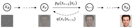
Figure 1. Flowchart of the diffusion model architecture.

In the forward process, the model corrupts an original image by incrementally adding Gaussian noise over 1000 steps. At each step, random noise sampled from a standard Gaussian distribution is applied together with the corresponding time step r, and Gaussian noise is incrementally added according to a predefined variance schedule; the noise-addition process is defined in Equation (1).

$$x_r=\sqrt{{\overline{\alpha }}_r}{x}_0+\sqrt{1-{\overline{\alpha }}_r}ϵ,\hspace{1em}{\overline{\alpha }}_r={\displaystyle \prod _{s=1}^r(1-{\beta }_s)}$$

(1)

where I denotes the identity matrix, ${\beta }_s$ denotes the variance at step s, ${\alpha }_r$ denotes the proportion of the original data retained at step r, and ${\overline{\alpha }}_r$ denotes the cumulative retention from the initial state through step r. The model generalizes this operation across the entire noise-addition process; the procedure is defined in Equation (2).

$$q(x_r\mid x_0)=\mathcal{N}(x_r;\sqrt{{\alpha }_r}{x}_0,(1-{\overline{\alpha }}_r)I)$$

(2)

When the time step r = R, the corruption approaches a standard Gaussian distribution. The image becomes completely noise-dominated.

In the reverse process, the model performs 1000 denoising steps. At each denoising step, the network predicts the noise component associated with the current time step t; this prediction is compared with the true noise $ϵ$, and the resulting loss is backpropagated to update the network parameters, thereby removing noise from the image. Through this procedure, the model learns the underlying image data distribution and ultimately recovers the denoised image to the original; the loss function is defined in Equation (3).

$$L_{\mathit{diff}}=E_{r,x_0,ϵ}{‖ϵ-{ϵ}_{\theta }\left(\sqrt{{\alpha }_r}{x}_0+\sqrt{1-{\overline{\alpha }}_r}ϵ,r\right)‖}^2$$

(3)

where ${ϵ}_{\theta }\left(x_r,r\right)$ denotes the noise predicted by the network, $\theta$ represents the learnable parameters, and $ϵ$ is the real noise. Classical diffusion models typically employ a U-Net as the backbone network for noise estimation. This network takes the image and its conditional information as input and consists of multiple levels of residual-connected up-sampling layers, down-sampling layers, and intermediate layers. Attention mechanisms are integrated across these layers, enabling the diffusion model to effectively capture multi-scale structures and fine-grained details of the image during the generation process.

2.2. CLE Diffusion

CLE Diffusion is a conditional diffusion model designed to adjust the brightness of low-light images. The model takes a low-light image as input and uses the brightness level derived from a corresponding high-light image as guidance for enhancement. During the forward process, noise is added to the high-light image based on a predefined schedule. Concurrently, chromatic and SNR maps are computed from the low-light image to serve as auxiliary information. These maps are concatenated with the low-light image and fed into a U-Net for reverse denoising. The brightness level from the high-light image is injected as a conditioning signal at each denoising step, enabling precise control over brightness enhancement. After multiple iterative denoising steps, the model generates a brightness-improved version of the low-light image. This approach achieves fine-grained regulation throughout the enhancement process. The overall framework is illustrated in Figure 2.

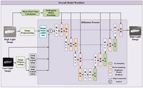
Figure 2. Architecture of the CLE Diffusion model.

During training, CLE Diffusion adds noise to the target high-light image y according to a predefined noise schedule, resulting in a fully corrupted version. This noisy image is then concatenated with the low-light image x, the chromatic map $C(x)$, and the SNR map $S(x)$. The combined input is passed into the U-Net. By incorporating the two auxiliary maps, the model enhances the generated image with improved chromatic details and noise-level structures. The computation of $C(x)$ is defined in Equation (4).

$$C(x)={\displaystyle \frac{x}{x_{\mathit{max}}}}=\left[{\displaystyle \frac{x_r}{x_{r,\mathit{max}}}},{\displaystyle \frac{x_g}{x_{g,\mathit{max}}}},{\displaystyle \frac{x_b}{x_{b,\mathit{max}}}}\right]$$

(4)

where $x_r$, $x_g$ and $x_b$ denote the pixel values of the red, green, and blue channels, respectively, after decomposing the visible-light image into three channels. $x_{\mathit{max}}$ represents the maximum pixel value for each color channel, which is categorized into three channels: $x_{r,\mathit{max}}$, $x_{g,\mathit{max}}$ and $x_{b,\mathit{max}}$. The calculation formula $S(x)$ is defined in Equation (5).

$$S(x)={\displaystyle \frac{F(x)}{|x-F(x)+ϵ|}}$$

(5)

where $ϵ$ denotes the noise imposed by the diffusion model, and $F(x)$ denotes the low-pass filter. After the image is fed into the U-Net, the model first computes the mean pixel value of the high-illumination image y, yielding a two-dimensional scalar brightness level λ. This λ is then introduced as a control condition into the brightness branch of each ResBlock within the U-Net down-sampling layers. Inside the brightness branch, λ undergoes normalization and orthogonal matrix sampling, followed by mapping through two MLP layers into a set of affine parameters $\left(\gamma ,\beta \right)$. These parameters are applied to the intermediate feature map $F$ from the previous layer by channel-wise affine transformation, producing the feature map $F_l$ with integrated brightness information. The computation is defined in Equation (6).

$$F_l=\gamma \cdot F+\beta$$

(6)

During the iterative denoising process, the model gradually learns the mapping between the brightness level λ and the corresponding image brightness features through the affine computation. This enables precise control over the brightness enhancement effect.

In CLE Diffusion, the model utilizes a composite loss function $L_{\mathit{aux}}$ for joint optimization. This loss function integrates multiple loss terms, specifically comprising five components: mean squared error loss $L_{\mathit{simple}}$, brightness loss $L_{\mathit{br}}$, angle color loss $L_{\mathit{col}}$, SSIM loss $L_{\mathit{ssim}}$, and perceptual loss $L_{\mathit{lpips}}$. The formulation of $L_{\mathit{aux}}$ is defined in Equation (7).

$$L_{\mathit{aux}}=L_{\mathit{simple}}+W_{\mathit{br}}{L}_{\mathit{br}}+W_{\mathit{col}}{L}_{\mathit{col}}+W_{\mathit{ssim}}{L}_{\mathit{ssim}}+W_{\mathit{lpips}}{L}_{\mathit{lpips}}$$

(7)

where $W_{\mathit{br}}$, $W_{\mathit{col}}$, $W_{\mathit{ssim}}$ and $W_{\mathit{lpips}}$ denote the weight coefficients for their respective loss terms.

2.3. TSP-CLE Diffusion Model

To address the dual challenges of modeling the temporal-brightness correlation in infrared images and the problem of edge blurring, a multi-temporal infrared image generation algorithm based on an improved CLE Diffusion is proposed. The method employs a low-light enhancement diffusion model to capture temporal brightness variations in infrared images. A temporal control module is incorporated to guide the model in learning the correspondence between time and brightness, while a structural consistency module is introduced to reinforce edge information and enhance generation quality.

In the forward noising process, the model computes chromatic and SNR maps from the target image. By concatenating noisy images with the different time target image, its chromatic map, and its SNR map, the model gains the ability to control structural fidelity and suppress low-SNR artifacts in infrared data. In the reverse denoising process, the core U-Net architecture is enhanced with two key modules. Temporal control module encodes temporal information using sinusoidal functions and employs FiLM-based feature modulation to jointly model time and brightness, thereby improving temporal feature accuracy. The structural consistency module uses multi-scale edge features from the target image as conditional inputs and introduces a structure-preserving attention mechanism to enhance edge representation and improve detail fidelity. Finally, the improved U-Net performs iterative denoising to generate images at arbitrary timesteps from multi-temporal inputs. The overall framework is illustrated in Figure 3, where * indicates the feature map containing only half of the channels.

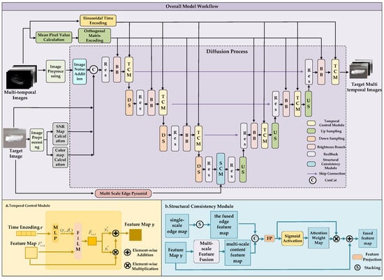
Figure 3. Architecture of the TSP-CLE Diffusion model. (a) Temporal Control Module; (b) Structural Consistency Module.

2.3.1. Time Encoding and Temporal Control Module

Traditional low-light enhancement models can generate multi-temporal images through brightness adjustment. However, their control mechanisms typically rely on manually selected reference images for illumination guidance. To overcome this lack of an autonomous temporal–brightness mapping, we introduce a periodic temporal encoding scheme based on sine and cosine functions as a conditional input. We then construct a temporal control module using FiLM-based feature modulation, which guides the model to learn the nonlinear mapping between brightness and temporal features. This approach enables precise control over the temporal characteristics of the generated images and reduces brightness deviations.

Sinusoidal Time Encoding

To capture the periodic nature of temporal information, the model encodes it using sine and cosine functions. By mapping each timestamp onto a unit circle, we convert time into a phase angle. The projections of this angle onto the x and y axes are then used as components to generate a two-dimensional vector representing temporal information. Compared with traditional discrete encoding methods, such as one-hot or segmented encoding, the sinusoidal encoding preserves temporal continuity. It also effectively represents the periodic characteristics of temporal data, including the cyclic pattern of day and night. The encoding is defined in Equation (8).

$$e=\mathit{Encoder}(t)=\left[\mathit{sin}\left({\displaystyle \frac{2\pi t}{T}}\right),\mathit{cos}\left({\displaystyle \frac{2\pi t}{T}}\right)\right]$$

(8)

where t denotes the timestamp of the image, and T denotes the length of the temporal period. In this model, a 24-h cycle is adopted based on the hourly system. The encoding maps the timestamp to a continuous interval of [0, 2π], aligning the period of the sine and cosine functions with T. As t increases, the encoding values repeat for each integer multiple of T. This reflects the 24-h temporal cycle and naturally captures periodic characteristics.

Temporal Control Module

To address the limitations of the baseline CLE Diffusion model, specifically its inability to learn temporal information, reliance on manually selected images for brightness control, and the difficulty in conditioning the model with encoded temporal constraints, this study employs a joint brightness-time modeling strategy. This approach integrates temporal encoding into the model training process. To this end, a temporal control module is introduced into the brightness branch of each residual block in the U-Net. The module takes the brightness feature map and the sinusoidal time encoding e as inputs. It integrates temporal information while enabling joint learning with brightness features, thereby establishing an effective mapping between the two. The structure of the module is illustrated in Figure 3a. The module first passes e through a three-layer fully connected network to generate channel-wise affine parameters $({\gamma }_c,{\beta }_c)$. The dimensions of these parameters are adaptively adjusted by the MLP to match the dimensions of feature map $F_{c,i,j}^{\prime }$ output from the U-Net’s brightness branch, facilitating subsequent modulation calculations. The computation is defined in Equation (9).

$$({\gamma }_c,{\beta }_c)=\mathit{MLP}(e)=W_2\mathit{ReLU}\left(W_{1}e+b_1\right)+b_2$$

(9)

where $W_1$ and $W_2$ denote the weight matrices, B₁ and B₂ denote the bias vectors, and ReLU denotes the nonlinear activation function. The affine parameters $({\gamma }_c,{\beta }_c)$ are applied to the feature map $F_{c,i,j}^{\prime }$ output from the brightness branch. Channel-wise scaling and shifting are performed, and the computation is defined in Equation (10).

$${\tilde{F}}_{c,i,j}={\gamma }_c\cdot F_{c,i,j}^{\prime }+{\beta }_c$$

(10)

After the scaling and shifting of temporal features, the output feature map ${\tilde{F}}_{c,i,j}$ is evenly split along the channel axis into $y_1^{*}$ and $y_2^{*}$. $y_1^{*}$ is first multiplied element-wise with the feature map from the brightness branch. $y_2^{*}$ is then added element-wise to the result. In this way, new modulated information is integrated while preserving the original details. The computation is defined in Equation (11).

$$y=F_{c,i,j}^{\prime }\otimes y_1^{*}\oplus y_2^{*}$$

(11)

Through this design, the temporal control module guides the network to learn the global brightness variation in images over time. It enables precise control of the multi-temporal image generation process.

2.3.2. Multi-Scale Edge Pyramid and Structural Consistency Module

Due to the multi-step iterative denoising mechanism of diffusion models, errors tend to accumulate during generation, often resulting in blurred edges. To address this issue, we design a multi-scale edge pyramid to extract edge information at different scales. We then propose a structural consistency module, based on a structure-preserving attention mechanism, which is embedded into the intermediate layers of the U-Net. In the deeper network layers, this module enhances edge representation by leveraging high-level semantic information while suppressing noise. The incorporation of multi-scale edge information strengthens edge feature learning, which helps reduce the uncertainty in diffusion models and improves the overall quality of the generated images.

Multi-Scale Edge Pyramid

The multi-scale edge pyramid is a variant of the multi-scale image pyramid. It combines multi-resolution analysis with edge detection to extract edge features at different scales. Coarse edge maps capture global structures, while fine edge maps focus on detailed information. After extraction, all edge maps are up-sampled to the original resolution and concatenated along the channel dimension, forming a unified representation that integrates multi-level edge information. This design enhances the model’s ability to perceive structural boundaries across scales, thereby improving the structural consistency of generated images. By strengthening edge feature learning, it reduces the uncertainty in the diffusion process and further improves the final image quality. The structure is illustrated in Figure 4.

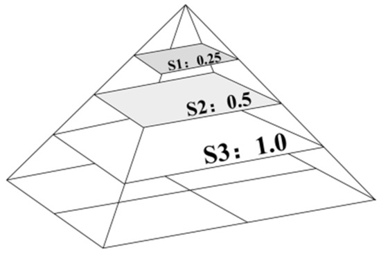
Figure 4. Multi-scale edge pyramid.

In this study, the target image I is down-sampled to three scales: {1.0, 0.5, 0.25}. Canny edge detection is then applied at each scale. The results are up-sampled back to the original image size using bilinear interpolation. The computation is defined in Equation (12).

$$E_i=\mathit{Resize}(\mathit{Canny}(\mathit{Resize}(I,s_i)),H,W)$$

(12)

where i denotes the scale. The three edge maps are stacked along the channel dimension to form the edge pyramid tensor. After normalization and bilinear interpolation down-sampling, an edge pyramid feature map $E_{\mathit{down}}$ is obtained with the same size as the intermediate feature maps of the U-Net. This feature map $E_{\mathit{down}}$ is used as the module input. The computation is defined in Equation (13).

$$E_{down}=\mathit{Resize}\left({\displaystyle \frac{\left[E_{1.0};E_{0.5};E_{0.25}\right]}{255}},(H_f,W_f)\right)$$

(13)

where $H_f$ and $W_f$ denote the height and width of the intermediate feature maps in the U-Net layers.

Structural Consistency Module

Integrating the temporal control module enables the model to adaptively regulate image brightness. However, this adjustment mechanism often results in the coverage of target edges. Specifically, brightness adjustments tend to spill over into adjacent regions where no modification is required. Consequently, this leads to a degradation of edge sharpness. To address the issue of edge blurring in infrared image generation caused by error accumulation, a structure consistency module is designed based on the structure-preserving attention mechanism. The module enhances the edge details of the generated images. It takes the edge pyramid feature $E_{\mathit{down}}$ as input. The structure-preserving attention mechanism integrates edge structural information with multi-scale content features. It extracts features from intermediate maps with different receptive fields. These features are used to compute attention with the edge feature maps. The process fuses multi-scale edge information into the feature representations. During generation, the module attends to global structures and shape details with precision. This improves the network’s ability to capture and preserve spatial relations. It reduces the shift in attention regions and strengthens the representation of edge information. The workflow of the module is illustrated in Figure 3b.

The module first applies three receptive fields of different sizes to the feature map F from the previous layer. This produces the multi-scale content feature $F_{\mathit{ms}}$. The computation of $F_{\mathit{ms}}$ is defined in Equation (14).

$$F_{\mathit{ms}}=\mathit{Concat}\left[{\mathit{Conv}}_{1\times 1}(F),{\mathit{Conv}}_{3\times 3}(F),{\mathit{Conv}}_{5\times 5}(F)\right]$$

(14)

At the same time, each single-scale edge map from $E_{\mathit{down}}$ is stacked along the channel dimension. After channel concatenation, a 1 × 1 convolution is applied for dimensionality reduction. The fused edge feature is obtained. The computation is defined in Equation (15).

$$E_{\mathit{fus}}={\mathit{Conv}}_{1\times 1}\left(\mathit{Concat}\left[E_1,E_2,E_3\right]\right)$$

(15)

The multi-scale content feature $F_{\mathit{ms}}$ and the fused edge feature $E_{\mathit{fus}}$ are concatenated. A 1 × 1 convolution is applied for feature projection, followed by activation with the Sigmoid function. The spatial attention weight map M is generated. The computation is defined in Equation (16).

$$M=\sigma \left({\mathit{Conv}}_{1\times 1}\left(\mathit{Concat}\left[F_{\mathit{ms}},E_{\mathit{fus}}\right]\right)\right)$$

(16)

Finally, the attention weight map M is used to weight the projected features. A fused residual is introduced, producing the final fused feature map Y. The computation is defined in Equation (17).

$$Y={\mathit{Conv}}_{1\times 1}\left(\mathit{Concat}\left[F_{\mathit{ms}},E_{\mathit{fus}}\right]\right)\otimes M+F$$

(17)

The structural consistency module explicitly incorporates multi-scale edge priors at the deepest layer of the network. It emphasizes key structural locations through a combination of attention weighting and residual fusion. This design significantly enhances the model’s sensitivity to geometric structures and edge details.

2.3.3. Loss Function

Based on the CLE Diffusion loss, an edge consistency loss is introduced to reinforce edge information. The Canny operator denotes the extraction of edge maps from both the generated image and the reference image, and the $L_1$ norm denotes the measurement of their difference. The loss function is defined in Equation (18).

$$L_{\mathit{edge}}={‖E_{\mathit{pyr}}(I_{\mathit{pred}})-E_{\mathit{pyr}}(I_{\mathit{gt}})‖}_1$$

(18)

where $E_{\mathit{pyr}}(\cdot )$ denotes the multi-scale edge pyramid, $I_{\mathit{pred}}$ denotes the enhanced image, and $I_{\mathit{gt}}$ denotes the reference image. The edge consistency loss encourages alignment of the output image with the reference image in edge distribution, facilitating sharper and more structurally accurate results. Introducing the edge consistency loss improves detail reconstruction accuracy without introducing additional artifacts. After incorporating this loss, the overall loss function of the model is defined in Equation (19).

$$L_{\mathit{all}}=L_{\mathit{aux}}+W_{\mathit{edge}}{L}_{\mathit{edge}}$$

(19)

where $L_{\mathit{aux}}$ denotes the CLE Diffusion loss, and $W_{\mathit{edge}}$ represents the weight of the edge consistency loss.

3. Experimental Results and Analysis

3.1. Experimental Setup

3.1.1. Datasets and Parameter Settings

The algorithm’s effectiveness is validated from two dimensions: generation quality and temporal feature fidelity. Experiments were conducted on the public “Year-long hourly façade photos of a university building” [22] visible-light dataset, the public “long-term thermal drift” infrared dataset [23] and our self-constructed Multi-Temporal Infrared Image Dataset (MTIID), captured by an infrared thermal imager. The public dataset contains 9596 façade images of a university building in Barcelona, Spain, including 6414 west-facing and 3182 east-facing images. All images were originally captured at 1290 × 1080 resolution using two identical GoPro Hero 10 cameras. The images were resized to 640 × 480 resolution to prevent system memory overflow. To ensure data consistency, only image pairs captured at different times on the same date were selected for testing. These pairs were manually filtered to maintain identical window-opening states. The morphological variations in the datasets are illustrated in Figure 5.

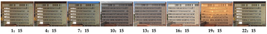
Figure 5. Illustration of the year-long hourly façade photos of a university building dataset.

The long-term thermal drift dataset was collected at the Aalborg Harbor front in Denmark, spanning an eight-month period from January to August 2023. The dataset was captured using a Hikvision DS-2TD2235D-25/50 thermal camera (Hikvision, Hangzhou, China). The sampling protocol involved 2-min recording sessions at 30-min intervals throughout the day, yielding approximately 1920 video clips. All videos are saved in 8-bit grayscale.mp4 format with a resolution of 288 × 384 pixels. The dataset captures diverse environmental conditions (e.g., rain, snow, fog) and various dynamic objects, including dense crowds, vehicles, and bicycles. It is specifically designed to facilitate the study of thermal drift, investigate environmental impact, and benchmark robust thermal analysis algorithms. The morphological variations in the datasets are illustrated in Figure 6.

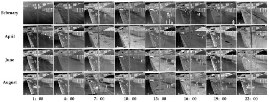
Figure 6. Illustration of the long-term thermal drift dataset.

Our MTIID was collected at the front square of the School of Science, Shenyang Ligong University. A total of 7680 infrared images were captured, each with a resolution of 640 × 480. The dataset includes eight specific targets belonging to three categories: airplanes, tanks, and vehicles. All targets are scaled-down replicas of actual military equipment with accurate proportions, rather than real combat assets. For each target, infrared images were captured at six different times of day: 01:00, 05:00, 09:00, 13:00, 17:00, and 21:00. The timestamps 01:00, 09:00, 13:00, and 21:00 were chosen to represent relatively stable thermodynamic states. In contrast, 05:00 (sunrise) and 17:00 (sunset) serve as critical transitional periods. These moments involve rapid changes in solar altitude and pronounced thermal inertia effects. Characterized by sharp fluctuations in temperature gradients, they demonstrate environmental specificity and temporal complexity in thermal imaging analysis. At each time point, 80 images were taken from various viewing angles. To prevent overfitting during model training, data augmentation was applied. The images were randomly cropped to 128 × 128, horizontally and vertically flipped, and normalized to stabilize the training process. The appearance of different target models in the dataset is illustrated in Figure 7.

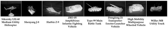
Figure 7. Illustration of the self-constructed dataset.

All experiments are conducted on a computing platform equipped with an NVIDIA GeForce RTX 3090 GPU (NVIDIA, Santa Clara, CA, USA). The operating system is Windows 11, and the deep learning framework is PyTorch. The environment configuration includes Python 3.10 and CUDA 12.1. The parallel computing capability of the GPU is fully utilized to maximize training efficiency.

The model is trained using the AdamW optimizer. The initial learning rate is set to $5\times {10}^{-5}$, and the weight decay is set to $1\times {10}^{-4}$. The training process comprises a total of 12,000 epochs with a batch size of 4. In the loss function, the weights $W_{\mathit{br}}$, $W_{\mathit{col}}$, $W_{\mathit{ssim}}$, $W_{\mathit{lpips}}$, and $W_{\mathit{edge}}$ are set to 20, 100, 2.83, 50, and 5, respectively.

3.1.2. Evaluation Metrics

To evaluate the image quality and temporal fidelity of the generated results, SSIM, PSNR, LPIPS, maximum amplitude spectrum value and direct current component peak $V_{\mathit{DC}}$ are adopted as evaluation metrics. These metrics are used to assess the performance of different models on the public dataset and our MTIID. SSIM, PSNR, and LPIPS are commonly used indicators for evaluating the quality of both visible-light and infrared images. The maximum amplitude spectrum value and direct current component peak are introduced from a physical perspective to measure the temporal fidelity of generated infrared images in the frequency and time domains. Specifically, the maximum amplitude spectrum value reflects the similarity of low-frequency information, such as brightness and structural details of infrared images. The calculation is expressed in Equation (20).

$$\mathit{max}\text{\_}\mathit{magnitude}=\max \left|\mathit{FFT}2\{f(x,y)\}\right|$$

(20)

where $f(x,y)$ denotes the gray value of the pixel located at the x row and y column of the image, and $\mathit{FFT}2\{\cdot \}$ represents the two-dimensional fast Fourier transform.

The direct current component peak is derived from the maximum amplitude spectrum value. It is proportional to the global brightness distribution of the infrared image in the time domain and reflects the similarity of average brightness among different infrared images. The calculation is expressed in Equation (21).

$$V_{\mathit{DC}}={\displaystyle \frac{\max (|X(f)|)}{N}}$$

(21)

where f denotes the frequency, $X(\cdot )$ represents the Fourier transform, and N denotes the number of points in the Fast Fourier Transform.

3.2. Comparative Analysis with SOTA Methods

To verify the effectiveness of the proposed method, we select several low-light enhancement models and remote sensing image multi-temporal generation models for comparison, including RetinexNet [24], KinD++ [25], HWMNet [26], Zero-DCE [27], LLFlow [20], Changen [15], and ChangeDiff [28], as well as the baseline model, CLE Diffusion. Among these, RetinexNet, KinD++, HWMNet, and Zero-DCE are static image enhancement algorithms, LLFlow is a dynamic frame enhancement algorithm, while Changen and ChangeDiff are visible light image multi-temporal generation algorithms.

3.2.1. Performance on the Public Visible-Light Dataset

To evaluate the model’s performance in visible-light image generation, comparative experiments are conducted on the public dataset. The experimental results are presented in Table 1.

Table 1. Model Comparison Results on Visible-Light Images.

	PSNR ↑	SSIM ↑	LPIPS ↓
RetinexNet [21]	7.58	0.30	0.53
HWMNet [23]	14.56	0.63	0.18
Zero-DCE [24]	11.93	0.72	0.24
LLFlow [19]	17.97	0.78	0.11
KinD++ [22]	19.25	0.84	0.12
Changen [14]	15.30	0.81	0.08
ChangeDiff [25]	13.04	0.70	0.20
CLE Diffusion [20]	22.65	0.84	0.18
TSP-CLE Diffusion	23.13	0.85	0.07

As shown in Table 1, TSP-CLE Diffusion outperforms all competing methods, achieving the highest PSNR and SSIM scores and the lowest LPIPS score. This indicates that the pixel-level differences between the generated and real images are minimal. The contrast and brightness of the generated images also closely align with the real images. Moreover, the low perceptual discrepancy shows a high degree of similarity in high-level visual features, such as texture and edge details.

We assessed the statistical significance of visual quality differences using PSNR, SSIM, and LPIPS on the Public Visible-Light Dataset, with 10 samples per model. A paired t-test compared the performance of various methods against the baseline, CLE Diffusion, on the identical test set. To visualize these results, we present a comparative chart using bar graphs to illustrate the means and standard deviations for each metric. Statistically significant improvements over the baseline are denoted by asterisks.

As shown in Figure 8, HWMNet, Zero-DCE, RetinexNet, and ChangeDiff show inferior performance across all three metrics compared to the baseline. This indicates that these models introduce substantial distortions and fail to preserve perceptual quality. Conversely, LLFlow, KinD++, and Changen present a more nuanced performance pattern. While they outperform the baseline in LPIPS (suggesting better perceptual quality), their PSNR and SSIM scores are lower. This discrepancy reflects deficiencies in pixel-level reconstruction accuracy and brightness distribution. In contrast, TSP-CLE Diffusion demonstrates the most balanced and superior overall performance. It exceeds the baseline across all metrics. This confirms its ability to preserve structural and perceptual quality, generating brightness characteristics that align accurately with real-world distributions.

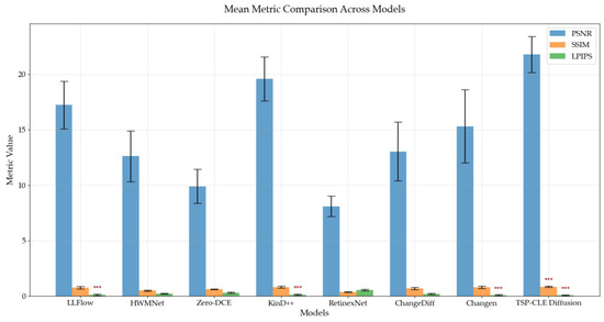
Figure 8. Paired t-test analysis of model metrics on the year-long hourly façade, where *** indicates significantly superior performance compared to the baseline model.

To further verify the generation capability of the proposed model on visible-light images, visual comparisons are conducted based on the results produced by different models. The analysis focuses on the enhancement of edge details and the generation of temporal characteristics. First, the generated images from each model are compared in terms of edge detail performance, and the results are shown in Figure 9. All input images correspond to 19:15, while the real images correspond to 13:15. The first row shows images captured on 29 September from the west side of the building, the second row shows images captured on 11 October from the west side, the third row shows images captured on 16 October from the east side, and the fourth row shows images captured on 22 October from the east side. Since lighting conditions vary across different dates due to factors such as weather and cloud coverage, images captured at the same time on different days are not completely identical in illumination.

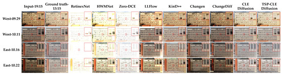
Figure 9. Model comparison of generation details on the year-long hourly façade.

As shown in Figure 9, RetinexNet, HWMNet, and Zero-DCE exhibit severe overexposure in their generated results, causing serious distortion in color and detail. LLFlow and KinD++ produce images whose colors are heavily influenced by the input images, resulting in noticeable color deviations from the real images. Changen and ChangeDiff exhibit over-sensitivity to the colors of input images. Furthermore, they fail to accurately estimate the required brightness and color adjustments, resulting in unnatural artifacts in certain areas. Consequently, this leads to a degradation of edge sharpness and detail fidelity in the generated images. Although CLE Diffusion generates colors close to the real images, it lacks sufficient detail. In contrast, TSP-CLE Diffusion can produce images whose brightness and color closely match the real images while preserving detail, achieving sharper edges in the generated images.

To further validate the temporal feature generation capability of each model, daytime and nighttime images are used as inputs to generate multi-temporal images. The generation results are shown in Figure 10 and Figure 11. The input images in Figure 10 are all daytime images at 14:15 on 6 October, while the input images in Figure 11 are all nighttime images at 23:15.

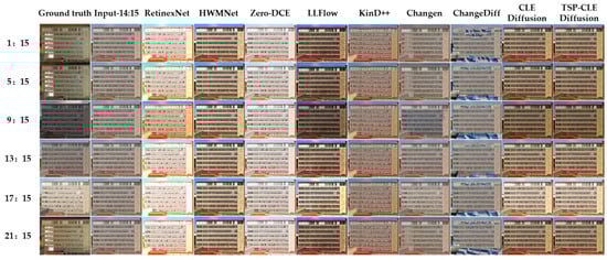
Figure 10. Comparison of multi-temporal generation results using daytime images from the year-long hourly façade photos of a university building dataset.

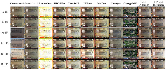
Figure 11. Comparison of multi-temporal generation results using nighttime images from the Year-long hourly façade photos of a university building dataset.

As shown in Figure 10 and Figure 11, the HWMNet, KinD++, and Zero-DCE models generate images with highly consistent brightness, failing to effectively distinguish temporal brightness variations. RetinexNet can adjust the generated brightness by calculating the luminance coefficient between the input and real images. However, the generated images are often over-exposed, and the performance on dark regions such as nighttime skies is poor, resulting in severe color deviations. LLFlow produces images that exhibit certain temporal differences, but the generated colors are frequently oversaturated. While Changen can learn certain brightness transition patterns, it remains influenced by input images, causing its brightness adjustments to deviate from real images. Similarly, ChangeDiff is constrained by input dependency and the stochastic nature of the diffusion model. A critical issue arises from semantic misinterpretation: for instance, the model may misclassify a building surface illuminated by night lights as soil. Consequently, applying the temporal transition of soil, it incorrectly synthesizes irrelevant jungle artifacts. This leads to a semantic discrepancy between the generated image and the actual scene. CLE Diffusion and TSP-CLE Diffusion generate images with natural brightness transitions, showing smooth temporal evolution.

A joint analysis of Figure 10 and Figure 11 reveals a common limitation: all models struggle to correctly render the colors of building walls and background during cross-time transitions, from daytime to nighttime or from nighttime to daytime. For instance, when the input is a nighttime image with the lights on the left side of the building illuminated, the generated images at all time points incorrectly retain these lights, which is inconsistent with actual daytime conditions. This phenomenon originates from the significant color differences between daytime and nighttime images, especially in key regions such as the sky, where color changes are drastic and exceed the generation capability of the models. This indicates that the models have limitations in generating images over long temporal spans. The generation results are therefore strongly influenced by the input image and still require further improvement.

3.2.2. Performance on the Public Infrared Dataset

To further evaluate the model’s performance in infrared image generation, comparative experiments are conducted on public infrared datasets, against existing low-light enhancement and multi-temporal generation models. The experimental results are presented in Table 2.

Table 2. Model Comparison Results on Public Infrared Images.

	PSNR ↑	SSIM ↑	LPIPS ↓
RetinexNet [21]	8.76	0.36	0.38
HWMNet [23]	12.09	0.49	0.34
Zero-DCE [24]	13.72	0.53	0.31
LLFlow [19]	14.78	0.50	0.30
KinD++ [22]	11.80	0.48	0.34
Changen [14]	14.59	0.52	0.26
ChangeDiff [25]	13.81	0.48	0.32
CLE Diffusion [20]	14.65	0.52	0.33
TSP-CLE Diffusion	15.93	0.55	0.30

As shown in Table 2, TSP-CLE Diffusion achieves the highest PSNR and SSIM scores alongside the lowest LPIPS score compared to the other models. This result indicates that the model more effectively captures temporal infrared features. It is less affected by noise in infrared images and generates more accurate detailed information.

To systematically evaluate the visual quality differences in multi-temporal infrared images generated by different models, this study adopts three key metrics: PSNR, SSIM, and LPIPS. Consistent with the evaluation of visible-light images, a paired sample t-test was employed for statistical significance analysis on the Public Infrared Dataset, with 24 samples per model. All comparative methods were benchmarked against the baseline method, CLE Diffusion, using metric results from the same test set. The analysis results are visualized using bar charts.

Figure 12 reveals that RetinexNet underperformed the baseline across all metrics, indicating a degradation in image quality. HWMNet and KinD++ showed relative weeknesses in SSIM, approaching statistically lower thresholds. Conversely, ChangeDiff, Changen, and Zero-DCE maintained moderate performance comparable to the baseline. Although LLFlow lacked statistical significance in LPIPS improvements, its value proximity to the threshold suggests perceptual gains. Notably, TSP-CLE Diffusion exhibited the best comprehensive performance, surpassing the baseline on all metrics. Its narrower error margins in PSNR and SSIM further indicate stable generation performance across different images.We further evaluate the visual results of each model to assess their capabilities in edge detail enhancement and temporal feature generation. First, a comparison of the generated image details is presented in Figure 13.

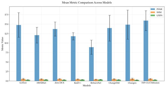
Figure 12. Paired t-test analysis of model metrics on the long-term thermal.

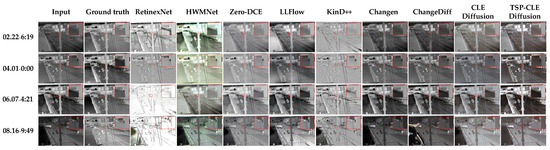
Figure 13. Model comparison of generation details on the long-term thermal drift dataset.

As shown in Figure 13, RetinexNet exhibits obvious infrared feature loss, with the generated images retaining only basic structural outlines. HWMNet demonstrates noticeable color distortion, generally manifesting as a greenish cast. Meanwhile, images generated by KinD++, LLFlow, and Zero-DCE suffer from reduced, with KinD++ also exhibiting color shift issues. The brightness distribution in outputs from Changen and ChangeDiff remains relatively close to the input images. This indicates these models are influenced by the luminance characteristics of input when processing both visible-light and infrared images. Although CLE Diffusion can generate relatively smooth outputs, it performs poorly in regions with drastic brightness variations. This leads to differences compared to the real images. In contrast, TSP-CLE Diffusion, incorporating an improved structural consistency module, demonstrates excellent performance in preserving object edges and details. Furthermore, it achieves precise adjustments across different brightness regions, enhancing inter-regional brightness contrast and overall image quality.

To further validate the temporal feature generation capability of each model, infrared images captured at a fixed time point are employed as inputs to generate multi-temporal images. Specifically, the input images were all taken at 00:00, and the generation results are shown in Figure 14.

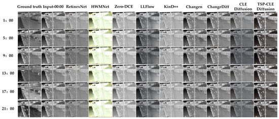
Figure 14. Comparison of multi-temporal generation results from the long-term thermal.

As shown in Figure 14, RetinexNet exhibits detail loss in its temporal generation results. However, compared to the near-complete thermal feature loss observed in the first two rows of Figure 13, the model retains key thermal features in the scenario shown in Figure 14. This difference is attributed to RetinexNet’s enhancement mechanism where intensity is controlled by an internal parameter, μ, dependent on the average brightness difference between the input and real images. A larger μ results in high enhancement intensity, leading to over-enhancement or loss of thermal features, while a smaller μ yields weaker enhancement, thus preserving more original thermal features. The results from KinD++, Zero-DCE, and HWMNet fail to capture temporal variation, with KinD++ also exhibiting information loss. This indicates these models struggle to learn subtle brightness changes in multi-temporal scene-level infrared images. While LLFlow and CLE Diffusion show brightness changes, their outputs suffer from edge blurring, resulting in reduced image quality. Although Changen and ChangeDiff adjust inputs based on real images from different times, they tend to prioritize changes over alterations in infrared features. For example, when generating street pedestrian images at 13:00, despite aligning with scene content patterns, they fail to reflect the corresponding changes in infrared features. In contrast, TSP-CLE Diffusion shows brightness differences across all six time points, yielding images with sharper edges. However, similar to its performance on visible-light images, the model faces challenges in achieving targeted brightness adjustments in scenes with complex regional brightness distributions. This highlights limitations in scene-level infrared image generation that require further optimization.

3.2.3. Performance on Our Infrared MTIID

To evaluate the model’s performance in infrared image generation, comparative experiments are conducted on our MTIID against existing low-light image enhancement models and multi-temporal models. The experimental results are presented in Table 3.

Table 3. Model Comparison Results on Our Infrared Images.

	PSNR ↑	SSIM ↑	LPIPS ↓
RetinexNet [21]	15.72	0.35	0.37
HWMNet [23]	15.14	0.39	0.30
Zero-DCE [24]	14.87	0.46	0.32
LLFlow [19]	14.67	0.35	0.31
KinD++ [22]	14.52	0.45	0.31
Changen [14]	12.63	0.47	0.39
ChangeDiff [25]	11.14	0.38	0.38
CLE Diffusion [20]	16.87	0.39	0.28
TSP-CLE Diffusion	16.97	0.51	0.19

As shown in Table 3, TSP-CLE Diffusion achieves the highest PSNR and SSIM scores and the lowest LPIPS score compared to the other models. This result indicates that the model more effectively captures temporal infrared features. It is less affected by noise in infrared images and generates more accurate detailed information.

To evaluate the visual quality differences in the generated multi-temporal infrared images, this study conducted a statistical significance analysis on three key metrics: PSNR, SSIM, and LPIPS, using the MTIID with 48 samples per model. Following the same procedure as for visible-light images, a paired sample t-test was used to compare the comparative methods against the baseline, CLE Diffusion, on the same test set. The analysis results are presented as bar charts.

As shown in Figure 15, LLFlow, KinD++, HWMNet, Zero-DCE, RetinexNet, and ChangeDiff exhibit inferior performance compared to the baseline across all three metrics, suggesting a limited capacity to capture the temporal characteristics of infrared images. These models show differences from the baseline (CLE Diffusion) in both pixel-level fidelity and perceptual quality. Changen, however, presents a distinct case: it achieves a statistically significant improvement in LPIPS, indicating a strong focus on perceptual quality. Nevertheless, its PSNR and SSIM scores remain lower than the baseline, reflecting insufficient modeling of pixel features and infrared brightness variations. In contrast, TSP-CLE Diffusion outperforms the baseline across all metrics. This confirms its superiority in preserving structural integrity and visual quality, enabling accurate generation of infrared brightness distribution. Furthermore, the narrower error bars for TSP-CLE Diffusion indicate enhanced stability across diverse test samples.

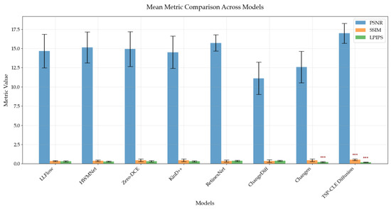
Figure 15. Paired t-test analysis of model metrics on the MTIID.

We further compare the visual results generated by each model to observe their edge detail enhancement and temporal feature generation capabilities. First, a comparison of generated image details is presented in Figure 16.

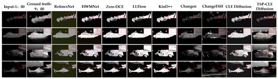
Figure 16. Model comparison of generation details on the MTIID.

As shown in Figure 16, RetinexNet generates images with severe noise interference, while HWMNet exhibits obvious color distortion and purple artifacts inside the targets. LLFlow, KinD++, Zero-DCE, and CLE Diffusion produce relatively smooth outputs, but they generally suffer from detail loss due to over-enhancement. The root cause of these issues lies in the design of traditional visible-light enhancement models, which process RGB channels in parallel. When transferred to single-channel infrared image generation, these models misinterpret the image SNR features and amplify them repeatedly, leading to ripple artifacts and oversaturation. While Changen and ChangeDiff avoid the over-enhancement phenomenon common in low-light enhancement models, they exhibit high dependency on input images and inconsistency in adjusting target brightness areas. Theoretically, this non-uniform adjustment characteristic aligns with the objectives of multi-temporal remote sensing generation, where local areas remain unchanged while only modifying terrain features that vary over time. However, when applied to infrared images with sparse targets, this characteristic leads to quality degradation, primarily driven by feature misinterpretation. In contrast, TSP-CLE Diffusion, through its improved diffusion mechanism, effectively suppresses ground noise while maintaining edge sharpness, making target edges and details clearer and demonstrating advantages in structural consistency and edge detail preservation.

To further validate the temporal feature generation capability of each model, infrared images from the same time point are used as input to generate multi-temporal images. The input images are all taken at 01:00, and the generation results are shown in Figure 17.

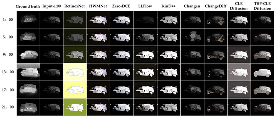
Figure 17. Comparison of multi-temporal generation results from MTIID.

As shown in Figure 17, RetinexNet, Zero-DCE, and HWMNet exhibit severe color or brightness deviations in temporal generation. Specifically, RetinexNet suffers from color collapse when generating images for high-brightness periods. In contrast, Zero-DCE and HWMNet apply the same enhancement level across all time points due to their training-data-based adaptive brightness adjustment mechanism, which prevents them from discriminating temporal features. LLFlow and KinD++ can leverage time-specific brightness information, but they remain insensitive to periods with similar brightness levels, producing nearly identical outputs and failing to capture subtle temporal variations. In multi-temporal generation tasks, Changen fails to capture fine-grained brightness distribution characteristics. Consequently, its brightness adjustment deviates from real scenes. Furthermore, the model’s brightness adjustment lacks selectivity. It non-selectively modifies background areas, leading to blurred target edges and geometric distortion. ChangeDiff performs relatively better in target-background separation. However, this is attributed to the low background brightness of the input images and the model’s dependency on input content. Additionally, since the model fails to decouple brightness information from structural features, the generated targets exhibit irregular textures and color artifacts. CLE Diffusion demonstrates sensitivity in high-brightness periods, but it over-enhances images during low-brightness periods. In contrast, TSP-CLE Diffusion exhibits significant and accurate brightness differences across all six time points, demonstrating a superior capability for multi-temporal brightness modeling and temporal consistency.

3.3. Evaluation of Physical Fidelity of Image Temporal Features

To verify the physical fidelity of temporal features in generated infrared images, we compare the maximum amplitude spectrum values of real and generated images at different time points. The comparison evaluates the similarity of low-frequency information in the frequency domain, with all generated images produced from a single input image taken at 1:00. By performing two-dimensional Fourier transform on multi-temporal images and applying spectral centering, we obtain three-dimensional spectral maps and their corresponding maximum amplitude spectrum values. Figure 17 visualizes these spectral maps of both real and generated images at each time point, with the maximum amplitude spectrum value indicated in the upper-left corner.

The results in Figure 18 show that the real and generated infrared images maintain a high degree of consistency in frequency-domain features at the same time point. This observation demonstrates that the target and background structural distributions of the generated images are highly similar to those of the real images, and that the infrared features remain consistent across different time points.

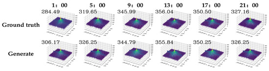
Figure 18. 3D Spectral visualization of real and generated images at each time.

To further evaluate the temporal feature fidelity of the generated images, we calculate the direct current component peak $V_{\mathit{DC}}$ based on the maximum amplitude of the image spectrum. By computing the Mean Absolute Error (MAE) and Failure Rate (FR) between the $V_{\mathit{DC}}$ values of the generated and real images, and visualizing these results in a dual-axis line chart, we can assess how closely the brightness of the generated images approximates the real images at each respective time point.

Figure 19 indicates that TSP-CLE Diffusion is prone to errors in only three transition cases ($13:00\to 09:00/17:00$ and $01:00\to 13:00$), with a total FR of 8.35%. The elevated MAE observed in the $01:00\to 13:00$ transition suggests a tendency towards over-enhancement when the input-target brightness gap is large. However, the model achieves a zero FR for target time of 01:00, 05:00, and 21:00, highlighting its robustness to model infrared characteristics. In contrast, the baseline CLE Diffusion has a FR of 38.89%. This performance gap underscores the improved stability and accuracy of the proposed method.

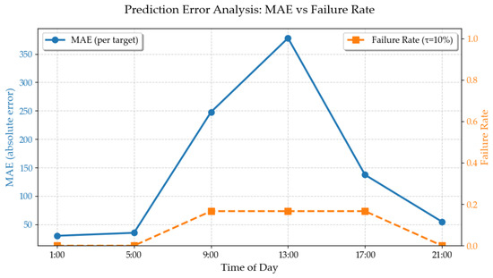
Figure 19. Error Curve and Failure Rate.

To verify the model’s generative capability under input images from different time points, we tested its ability to generate images at arbitrary time points using multi-temporal inputs. Figure 20 presents the experimental results, where the horizontal axis represents the generation time points and the vertical axis represents the input real image time points.

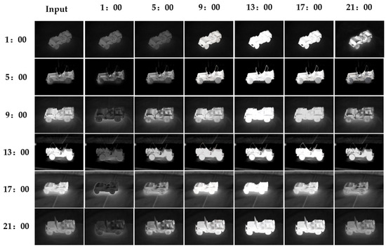
Figure 20. Examples of generated infrared images at each time.

The results in Figure 20 show that the generated images generally match the brightness of the original images and follow the temporal variation patterns. However, when using the high-brightness 13:00 image to generate lower-brightness images at 09:00 and 17:00, the generated results exhibit over-enhancement. This phenomenon arises from the bidirectional asymmetric nature of the model’s brightness adjustment mechanism. Low-light enhancement models are typically optimized for mappings from low to high brightness. When applied to high-to-low brightness mappings, the parameter space lacks convergence in the inverse direction, which easily results in brightness drift. Consequently, when performing slight brightness reduction based on high-brightness images, the model’s sensitivity to brightness gradients is insufficient, causing nonlinear changes in reduction magnitude and leading to inadequate brightness attenuation.

3.4. Ablation Study

To verify the effectiveness of the proposed temporal control module and structural consistency module, two ablation models are designed: T-CLE Diffusion, which incorporates only the temporal control module, and SP-CLE Diffusion, which incorporates only the structural consistency module. These models are evaluated on the MTIID and the long-term thermal drift dataset to assess the contribution of each module to image quality improvement. Table 4 and Table 5 present the results of the ablation experiments, where SSIM, PSNR, and LPIPS are used to quantitatively assess the performance of each model.

Table 4. Results of the Model Ablation Study on the MTIID.

	PSNR ↑	SSIM ↑	LPIPS ↓
CLE Diffusion	16.87	0.39	0.28
T-CLE Diffusion	16.03	0.48	0.21
SP-CLE Diffusion	16.50	0.48	0.20
TSP-CLE Diffusion	16.97	0.51	0.19

Table 5. Results of the Model Ablation Study on the Public Infrared Dataset.

	PSNR ↑	SSIM ↑	LPIPS ↓
CLE Diffusion	14.65	0.52	0.33
T-CLE Diffusion	15.28	0.52	0.32
SP-CLE Diffusion	15.64	0.53	0.32
TSP-CLE Diffusion	15.93	0.55	0.30

The experimental results indicate that TSP-CLE Diffusion achieves the best performance in PSNR, SSIM, and LPIPS. It is noteworthy that integrating either the temporal control module or the structural consistency module leads to a decrease in PSNR compared with TSP-CLE Diffusion. This decrease arises because each module, when acting independently, introduces mutually conflicting representation biases: Independently integrating the temporal control module enables the model to adjust the brightness distribution of generated images based on luminance conditions. This aligns the output more closely with real images, improving visual quality. Since SSIM is sensitive to brightness, these adjustments make images better align with human perception, thereby increasing SSIM. Simultaneously, the improved natural appearance reduced perceptual differences, leading to a lower LPIPS. However, brightness control can introduce pixel deviations, particularly in edge regions. Adjusting brightness can blur the distinction between pixels on both sides of an edge, resulting in blurred contours and, consequently, a decrease in PSNR. Conversely, independently introducing the structural consistency module enhances edge clarity and texture detail. Given SSIM’s focus on structural information, clearer edges directly boost SSIM. Furthermore, improved detail restoration enhances perceptual naturalness, causing LPIPS to decrease. However, edge enhancement modifies pixel values in target edge regions. Lacking temporal information, the model struggles to accurately determine the adjustment direction for pixel brightness. While it ensures distinct boundaries, this often leads to pixel-level differences against the real image, resulting in a decrease in PSNR. Therefore, the temporal control module focuses on brightness modulation over time, which can amplify noise and generate edge artifacts, while the structural consistency module emphasizes multi-scale edges and high-frequency details, which may cause brightness imbalance if applied without additional constraints. When the two modules operate collaboratively, the temporal control module suppresses brightness drift across time steps, providing a stable amplitude baseline for the structural consistency module. In turn, the structural consistency module corrects edge blurring and artifacts caused by temporal modulation. Together, the two modules achieve a critical balance between global brightness consistency and edge structure fidelity, ultimately enhancing overall structural consistency and perceptual quality.

Experimental results demonstrate that TSP-CLE Diffusion achieves the best performance on public infrared datasets in terms of PSNR, SSIM, and LPIPS. Notably, the complete model synergizes the temporal control and structural consistency modules. Unlike the ablation studies where individual modules led to pixel-level degradation, the full framework mitigates this trade-off, ensuring high fidelity. This indicates that the model exhibits good adaptability to public datasets.

Further analysis reveals why performance datasets. Compared to public datasets, MTIID contains images with more noise and camera instability, causing a general drop in performance metrics. Notably, when the ‘Willys MB Utility Truck’ data is excluded, both T-CLE and SP-CLE Diffusion outperform the baseline in PSNR. This suggests that the ‘Willys MB Utility Truck’ represents a corner case due to its unique material composition and low image quality. Models equipped with only a single module lack the ability to process such extreme data degradation, resulting in poorer generation quality for this specific target.

3.4.1. Visual Analysis of the Temporal Control Module

To evaluate the temporal feature generation accuracy of the temporal control module, we analyze the images generated by CLE Diffusion and T-CLE Diffusion against their corresponding real images. In the experiment, we select one model type from the dataset for each of the three target categories and generate grayscale histograms to compare differences among images across various grayscale ranges. The results are shown in Figure 21, Figure 22 and Figure 23, where both models generate images at 09:00 based on an input at 01:00.

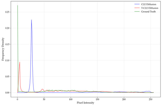
Figure 21. Grayscale histogram of the high mobility multipurpose wheeled vehicle.

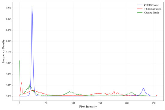
Figure 22. Grayscale histogram of the ZBD-05 amphibious infantry fighting vehicle.

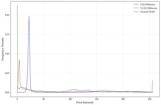
Figure 23. Grayscale histogram of the harbin Z-9.

As shown in Figure 21, Figure 22 and Figure 23, the grayscale distributions of real images exhibit a broad and diffuse pattern for each target category. While concentrated in the lower grayscale region, the distribution extends noticeably into the mid-to-high ranges, indicating the presence of multiple brightness levels and thermal regions in real-world scenarios. In contrast, the grayscale distribution of CLE Diffusion is heavily concentrated in the lower range, with a sharp peak and minimal presence in the mid-to-high regions. This suggests a significant deficiency in the model’s ability to represent high-brightness pixels. Although T-CLE Diffusion also shows a peak in the lower grayscale region, its distribution is broader and extends into the mid-to-high ranges. The overall shape of its curve aligns better with that of the real images. Therefore, compared to the baseline, T-CLE Diffusion achieves a better fit to the grayscale statistical distribution of real images. However, its performance in the high-brightness region indicates that further improvements are needed to enhance the generation accuracy of high-brightness pixels.

3.4.2. Visual Analysis of Structural Consistency Module

To evaluate the edge detail fidelity of the structural consistency module, we analyze the images generated by CLE Diffusion and SP-CLE Diffusion against their corresponding real images. In the experiments, we select one model type from the dataset for each of the three target categories and apply Canny edge detection to generate edge maps for visual comparison. The results are shown in Figure 24, where both models generate images at 09:00 based on an input at 01:00.

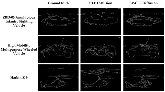
Figure 24. Infrared image edge image comparison.

As shown in Figure 24, for all targets, the edges of objects in infrared images generated by SP-CLE Diffusion are clearer and denser than those produced by CLE Diffusion. This indicates that SP-CLE Diffusion extracts more continuous and accurate edge lines on object surfaces and structural details, achieving superior reconstruction of surfaces such as tank tops, vehicle tops, and helicopter rotors, thereby demonstrating stronger edge detail restoration. In contrast, the edges in CLE Diffusion results are relatively sparse, with some structures appearing fragmented or blurred. Compared with real infrared images, it can be observed that the introduction of the structural consistency module effectively enhances the model’s ability to represent edge features, making the structural contours of the generated images closer to reality and thus validating the module’s effectiveness in improving the detail fidelity.

4. Conclusions

For the task of multi-temporal infrared image generation, this study proposes a novel image generation method based on CLE Diffusion, a low-light enhancement diffusion model. By constructing a temporal control module guided by time encoding, the model enhances its ability for adaptive temporal feature extraction, ensuring temporal consistency of the generated image sequence. In addition, a multi-scale edge pyramid and a structural consistency module are designed to strengthen edge clarity and detail fidelity. The collaborative effect of these two modules enables the generation of high-quality infrared images at arbitrary time points. Quantitative comparisons demonstrate that the model achieves superior performance on PSNR, SSIM, and LPIPS metrics. Analysis of the visualization results shows that the generated images exhibit noticeable temporal brightness variations that closely approximate real-world images, consistent with the temporal physical principles of infrared radiation. Ablation experiments further verify that the synergistic interaction between the temporal control and structural consistency modules has a significant impact on image generation quality.

Furthermore, our study identifies a universal limitation shared by all evaluate models, including TSP-CLE Diffusion, when processing scene-level images: they struggle to perform targeted brightness adjustments in areas with high spatial heterogeneity. Similarly to visible-light images, scene-level images are characterized by significant brightness differences and distinct regional segmentation. Existing models lack the ability to decouple and process brightness independently across different regions. Analysis of the dataset shows that the temporal brightness evolution in scene-level infrared images is complex. It cannot be simply characterized through overall brightness enhancement or reduction. Moreover, it is challenging to make reasonable inferences based on prior knowledge such as “higher brightness during daytime” or “lower brightness at night.” Therefore, enhancing capability for regional brightness adjustment is an important improvement direction for multi-temporal infrared image generation models. Strengthening the learning of brightness variation patterns in scene-level images will help apply these models to civilian fields, such as environmental monitoring and meteorological assessment.

References

- Zhang, W.; Zhang, Q.; Liu, S.; Pan, X.; Lu, X. A Spatial–Spectral Joint Attention Network for Change Detection in Multispectral Imagery. Remote Sens. 2022, 14, 3394. [Google Scholar] [CrossRef]
- Upadhyay, A.; Sharma, M.; Mukherjee, P.; Singhal, A.; Lall, B. A Comprehensive Survey on Synthetic Infrared Image Synthesis. Infrared Phys. Technol. 2025, 147, 105745. [Google Scholar] [CrossRef]
- Kniaz, V.V.; Gorbatsevich, V.S.; Mizginov, V.A. ThermalNet: A Deep Convolutional Network for Synthetic Thermal Image Generation. Int. Arch. Photogramm. Remote Sens. Spat. Inf. Sci. 2017, 42, 41–45. [Google Scholar] [CrossRef]
- Wang, F.; Zhao, H.; Peng, Y.; Fang, J.; Liu, P.; Zhang, R. MIIGAN: Mambas Make Strong GAN for Infrared Image Generation. Neural Netw. 2025, 193, 108021. [Google Scholar] [CrossRef] [PubMed]
- Li, B.; Ma, D.; He, F.; Zhang, Z.; Zhang, D.; Li, S. Infrared Image Generation Based on Visual State Space and Contrastive Learning. Remote Sens. 2024, 16, 3817. [Google Scholar] [CrossRef]
- Zhang, R.; Mu, C.; Xu, M.; Xu, L.; Shi, Q.; Wang, J. Synthetic IR Image Refinement Using Adversarial Learning with Bidirectional Mappings. IEEE Access 2019, 7, 153734–153750. [Google Scholar] [CrossRef]
- Gong, H.; Hu, Y.; Tang, S.; Ma, Y.; Xu, L. Multi-Time Infrared Image Generation Algorithm Based on DP-MAST Network. In Proceedings of the 2023 China Automation Congress, Chongqing, China, 17–19 November 2023; pp. 9020–9025. [Google Scholar]
- Dong, G.; Zhao, C.; Pan, X.; Basu, A. Learning Temporal Distribution and Spatial Correlation Toward Universal Moving Object Segmentation. IEEE Trans. Image Process. 2024, 33, 2447–2461. [Google Scholar] [CrossRef] [PubMed]
- Wang, Z.; Oates, T. Imaging Time-Series to Improve Classification and Imputation. In Proceedings of the 24th International Conference on Artificial Intelligence, Buenos Aires, Argentina, 25–31 July 2015; pp. 3939–3945. [Google Scholar]
- Liu, L.; Wang, Z. Encoding Temporal Markov Dynamics in Graph for Visualizing and Mining Time Series. In Proceedings of the AAAI Workshops, New Orleans, LA, USA, 2–3 February 2018; pp. 178–184. [Google Scholar]
- Chen, W.; Shi, K. A Deep Learning Framework for Time Series Classification using Relative Position Matrix and Convolutional Neural Network. Neurocomputing 2019, 359, 384–394. [Google Scholar] [CrossRef]
- Li, H.; Yu, S.; Principe, J. Causal Recurrent Variational Autoencoder for Medical Time Series Generation. In Proceedings of the AAAI Conference on Artificial Intelligence, Washington, DC, USA, 7–14 February 2023; Volume 37, pp. 8562–8570. [Google Scholar]
- Amirfakhrian, M.; Samavati, F.F. Variational-Based Spatial–Temporal Approximation of Images in Remote Sensing. Remote Sens. 2024, 16, 2349. [Google Scholar] [CrossRef]
- Kwak, G.H.; Park, N.W. Assessing the Potential of Multi-Temporal Conditional Generative Adversarial Networks in SAR-to-Optical Image Translation for Early-Stage Crop Monitoring. Remote Sens. 2024, 16, 1199. [Google Scholar] [CrossRef]
- Zheng, Z.; Tian, S.; Ma, A.; Zhang, L.; Zhong, Y. Scalable Multi-Temporal Remote Sensing Change Data Generation via Simulating Stochastic Change Process. In Proceedings of the IEEE/CVF International Conference on Computer Vision, Paris, France, 2–6 October 2023; pp. 21818–21827. [Google Scholar]
- Ho, J.; Jain, A.; Abbeel, P. Denoising Diffusion Probabilistic Models. Adv. Neural Inf. Process. Syst. 2020, 33, 6840–6851. [Google Scholar]
- Shen, L.; Kwok, J. Non-autoregressive Conditional Diffusion Models for Time Series Prediction. In Proceedings of the International Conference on Machine Learning, Honolulu, HI, USA, 23–29 July 2023; pp. 31016–31029. [Google Scholar]
- Aydin, K.; Hanna, J.; Borth, D. SAR-to-RGB Translation with Latent Diffusion for Earth Observation. arXiv 2025, arXiv:2504.11154. [Google Scholar]
- Khanna, S.; Liu, P.; Zhou, L.; Meng, C.; Rombach, R.; Burke, M.; Lobell, D.; Ermon, S. DiffusionSat: A Generative Foundation Model for Satellite Imagery. In Proceedings of the International Conference on Learning Representations, Vienna, Austria, 7–11 May 2024; pp. 19539–19557. [Google Scholar]
- Wang, Y.; Wan, R.; Yang, W.; Li, H.; Chau, L.P.; Kot, A.C. Low-Light Image Enhancement with Normalizing Flow. In Proceedings of the AAAI Conference on Artificial Intelligence, Virtual, 22 February–1 March 2022; Volume 36, pp. 2604–2612. [Google Scholar]
- Yin, Y.; Xu, D.; Tan, C.; Liu, P.; Zhao, Y.; Wei, Y. CLE Diffusion: Controllable Light Enhancement Diffusion Model. In Proceedings of the 31st ACM International Conference on Multimedia, Ottawa, ON, Canada, 29 October–3 November 2023; pp. 8145–8156. [Google Scholar]
- Roca-Musach, M.; Crespo Cabillo, I.; Coch, H. Image Dataset: Year-Long Hourly Façade Photos of a University Building. Data Brief 2024, 56, 110798. [Google Scholar] [CrossRef] [PubMed]
- Nikolov, I.A.; Philipsen, M.P.; Liu, J.; Dueholm, J.V.; Johansen, A.S.; Nasrollahi, K.; Moeslund, T.B. Seasons in Drift: A Long-Term Thermal Imaging Dataset for Studying Concept Drift. In Proceedings of the 35th Conference on Neural Information Processing Systems Track on Datasets and Benchmarks, Virtual, 6–14 December 2021; pp. 1–15. [Google Scholar]
- Wei, C.; Wang, W.; Yang, W.; Liu, J. Deep Retinex Decomposition for Low-Light Enhancement. In Proceedings of the British Machine Vision Conference, Newcastle, UK, 3–6 September 2018; pp. 451–462. [Google Scholar]
- Zhang, Y.; Guo, X.; Ma, J.; Liu, W.; Zhang, J. Beyond Brightening Low-light Images. Int. J. Comput. Vis. 2021, 129, 1013–1037. [Google Scholar] [CrossRef]
- Zhong, S.; Fu, L.; Zhang, F. Infrared Image Enhancement Using Convolutional Neural Networks for Auto-Driving. Appl. Sci. 2023, 13, 12581. [Google Scholar] [CrossRef]
- Guo, C.; Li, C.; Guo, J.; Loy, C.C.; Hou, J.; Kwong, S.; Cong, R. Zero-Reference Deep Curve Estimation for Low-Light Image Enhancement. In Proceedings of the IEEE/CVF Conference on Computer Vision and Pattern Recognition, Virtual, 14–19 June 2020; pp. 1780–1789. [Google Scholar]
- Zang, Q.; Yang, J.; Wang, S.; Zhao, D.; Yi, W.; Zhong, Z. ChangeDiff: A Multi-Temporal Change Detection Data Generator with Flexible Text Prompts via Diffusion Model. In Proceedings of the AAAI Conference on Artificial Intelligence, Philadelphia, PA, USA, 25 February–4 March 2025; Volume 39, pp. 9763–9771. [Google Scholar]
Disclaimer/Publisher’s Note: The statements, opinions and data contained in all publications are solely those of the individual author(s) and contributor(s) and not of MDPI and/or the editor(s). MDPI and/or the editor(s) disclaim responsibility for any injury to people or property resulting from any ideas, methods, instructions or products referred to in the content. |
© 2025 by the authors. Licensee MDPI, Basel, Switzerland. This article is an open access article distributed under the terms and conditions of the Creative Commons Attribution (CC BY) license (https://creativecommons.org/licenses/by/4.0/).