Real-Time Anomaly Detection Based on a Fast Recursive Kernel RX Algorithm

Abstract

Real-time anomaly detection has received wide attention in remote sensing image processing because many moving targets must be detected on a timely basis. A widely-used anomaly detection algorithm is the Reed-Xiaoli (RX) algorithm that was proposed by Reed and Yu. The kernel RX algorithm proposed by Kwon and Nasrabadi is a nonlinear version of the RX algorithm and outperforms the RX algorithm in terms of detection accuracy. However, the kernel RX algorithm is computationally more expensive. This paper presents a novel real-time anomaly detection framework based on the kernel RX algorithm. In the kernel RX detector, the inverse covariance matrix and the estimated mean of the background data in the kernel space are non-causal and computationally inefficient. In this work, a local causal sliding array window is used to ensure the causality of the detection system. Using the matrix inversion lemma and the Woodbury matrix identity, both the inverse covariance matrix and estimated mean can be recursively derived without extensive repetitive calculations, and, therefore, the real-time kernel RX detector can be implemented and processed pixel-by-pixel in real time. To substantiate its effectiveness and utility in real-time anomaly detection, real hyperspectral data sets are utilized for experiments.

1. Introduction

Hyperspectral imagery (HSI) can provide abundant spectral information to describe various ground materials due to its very high spectral resolution [1]. Anomaly detection, one of the main research areas, is of particular importance since it can uncover many subtle materials of which there is no prior knowledge or visualization for image analysts [2]. These types of materials generally appear as anomalies in hyperspectral images, such as special species in agriculture and ecology, rare minerals in geology, oil spills in water pollution, drug trafficking in law enforcement, man-made objects in battlefields, and tumors in medical imaging [3].

In HSI anomaly detection, the Reed-Xiaoli (RX) detector of Reed and Yu [4] is widely used and considered a baseline algorithm [5,6,7,8,9,10,11,12]. The well-known RX detector is the benchmark algorithm derived from a generalized likelihood ratio test for an unknown additive contrast signal in a multivariate Gaussian background. Complex ground material distributions have a negative impact on the RX detection since the RX detector only makes use of low-order statistics of hyperspectral data. To this issue, the kernel RX (KRX) algorithm [5], a nonlinear version of the RX algorithm, was proposed by Kwon and Nasrabadi. By mining the high-order correlation between spectral bands via a kernel function, the KRX detector (KRXD) provides better detection performance when original data samples are mixed in a non-linear model, as is always the case. Depending on the background information, KRXD can be divided into two types: global KRXD (GKRXD) and local KRXD (LKRXD). GKRXD calculates the Mahalanobis distance between a test pixel and global background information in the feature space, while LKRXD uses sliding windows to effectively detect local anomalous targets that could easily be overwhelmed in the global background. By virtue of a kernel trick [13], the KRX detector can be implemented using the dot products of input data in the original low dimensional space rather than in high dimensional space.

Recently, in applications of anomaly detection, there is an increasing interest concerning real-time and quick algorithms of anomaly detection in HSI [14,15,16]. It is particularly crucial since some moving targets, denoted by anomalies, need to be located in real time. Real-time processing also alleviates the need for data storage, system response time and the transmission of large amounts of hyperspectral data. Over the past few years, many real-time anomaly detection algorithms have been proposed to enable real-time or nearly real-time on-board processing in the literature [14,15,16,17,18,19,20,21,22,23,24,25,26]. In [14], computationally efficient anomaly detectors were developed and tested in the operating airborne platforms. In [17], the architecture for real-time global background data statistics evaluation is shown. To speed up processing time, real-time anomaly detection was successfully implemented on graphics processing units (GPUs) [21,22,23]. Subsequently, the real-time anomaly detectors based on efficient updating strategies were proposed and developed in [25,26]. Unfortunately, most of them are not actually real-time processors but simply fast algorithms. An anomaly detection algorithm for implementation in real time must meet the requirement of causality [16]. In other words, the data sample vectors used for data processing can only be those prior to the sample vector being visited, and any future sample vectors should not be involved in processing. By doing so, a real-time causal processing of anomaly detection was proposed in [15]. In this method, causal equations are derived and updated recursively. In [16,27], global real-time causal RX detectors (GRTC-RXD) and local real-time causal RX detectors (LRTC-RXD) based on different causal sliding windows were investigated. Both the GRTC-RXD and the LRTC-RXD use the Woodbury matrix identity to reduce computational complexity. While GRTC-RXD takes all data samples before the test pixel as background information, the LRTC-RXD only utilizes the background information in a local causal sliding window. However, these algorithms are designed based on RX detectors, where there is still a challenge of detection accuracy since they only use low-order statistics of hyperspectral data.

Therefore, this paper proposes a new framework of real-time anomaly detection based on the KRX algorithm that has better detection accuracy than RX algorithms. A local causal sliding array window is employed to ensure a causal detection system [27], thereby gaining an advantage in that the data samples are collected and detection is performed simultaneously. The matrix inversion lemma and Woodbury matrix identity are then combined to recursively update the inverse covariance matrix and the estimated mean of the background data in the kernel space. There is no need for the entire previously visited data sample vectors to be reprocessed, thereby speeding up real-time processing. After meeting the requirements of causality and efficiency, the kernel RX detector can be implemented and processed pixel-by-pixel in a real-time manner.

2. Methods

2.1. RX and KRX Anomaly Detector

Reed and Yu in [4] developed an RX detector that is a widely used anomaly detection algorithm in hyperspectral imaging. The RX algorithm calculates Mahalanobis distance between the data sample vector currently being detected and background data sample vectors. To exploit abundant nonlinear information of hyperspectral data, Kwon et al. proposed a KRX algorithm that has better separation performance between anomalies and the background by using kernel functions. In the following, we briefly describe the RX algorithm and the KRX algorithm.

2.1.1. RX Algorithm

Let each input spectral signal consisting of $l$ spectral bands be denoted by $x_i={[x_{1i},x_{2i},\dots ,x_{li}]}^T$. The two competing hypotheses that the RX-algorithm should distinguish are given by

$$\{\begin{array}{cc}{H}_0：\hspace{0.17em}x=n\hfill & \hfill (\mathrm{Target} \mathrm{absent})\\ H_1：\hspace{0.17em}x=as+n\hfill & \hfill (\mathrm{Target} \mathrm{present})\end{array}$$

(1)

where $a=0$ under $H_0$ and $a>0$ under $H_1$, $n$ is additive Gaussian noise, and $s$ is a vector that represents the spectral signature of the signal (target). The model assumes that the data are from two normal probability density functions with the same covariance matrix but different means. Under $H_0$, the data (background clutter) are modeled as $N(0,\mathbf{C})$, and under $H_1$ the data are modeled as $N(\mathsf{\mu },\mathbf{C})$. The RX detector, referred to as ${\mathsf{\delta }}^{{}_{\mathrm{RXD}}}\left(r\right)$, is specified by

$${\mathsf{\delta }}^{{}_{\mathrm{RXD}}}\left(r\right)={\left(r-\mathsf{\mu }\right)}^T{\mathbf{C}}^{-1}\left(r-\mathsf{\mu }\right)$$

(2)

where $\mathsf{\mu }$ is the background estimated mean and $\mathbf{C}$ is the background covariance matrix.

2.1.2. Kernel RX Algorithm

The KRX algorithm uses the same assumptions as those used in the RX algorithm, in other words, the mapped input data in the feature space now consists of two Gaussian distributions, thus modeling the two hypotheses as

$$\{\begin{array}{ll}{H}_{0\mathsf{\Phi }}：\mathsf{\Phi }(x)=n_{\mathsf{\Phi }}& \hfill (\mathrm{Target} \mathrm{absent})\\ H_{1\mathsf{\Phi }}：\mathsf{\Phi }(x)=a_{\mathsf{\Phi }}\mathsf{\Phi }(s)+n_{\mathsf{\Phi }}& \hfill (\mathrm{Target} \mathrm{present})\end{array}$$

(3)

where $a_{\mathsf{\Phi }}=0$ under ${{\rm H}}_{0\mathsf{\Phi }}$ and $a_{\mathsf{\Phi }}>0$ under ${{\rm H}}_{1\mathsf{\Phi }}$, $\mathsf{\Phi }(s)$ and $n_{\mathsf{\Phi }}$ represent target spectral signature and noise in the feature space, respectively. The corresponding KRX algorithm in the feature space is represented as

$${\mathsf{\delta }}^{{}_{\mathrm{KRXD}}}(\mathsf{\Phi }(r))={\left(\mathsf{\Phi }(r)-{\widehat{\mathsf{\mu }}}_{B\mathsf{\Phi }}\right)}^T{\widehat{K}}_{B\mathsf{\Phi }}^{-1}\left(\mathsf{\Phi }(r)-{\widehat{\mathsf{\mu }}}_{B\mathsf{\Phi }}\right)$$

(4)

where ${\widehat{\mathsf{\mu }}}_{B\mathsf{\Phi }}$ and ${\widehat{K}}_{B\mathsf{\Phi }}$ are the estimated mean and covariance matrix of the background data in the feature space, respectively. Through certain kernelization and derivation,

$${\mathbf{k}}_{\mathbf{r}}^T=k(\mathbf{r},{\mathbf{X}}_B)-(\frac{1}{N}{\displaystyle \sum _{i=1}^{N}k(\mathbf{r},{\mathbf{x}}_i)})$$

(5)

$${\mathbf{k}}_{\widehat{\mathsf{\mu }}}^T=(\frac{1}{N}{\displaystyle \sum _{i=1}^{N}k({\mathbf{x}}_i,{\mathbf{X}}_B)})-(\frac{1}{N^2}{\displaystyle \sum _{i=1}^N{\displaystyle \sum _{j=1}^{N}k({\mathbf{x}}_i,{\mathbf{x}}_j)}})$$

(6)

where ${\mathbf{X}}_B$ is the original background data including $N$ data sample vectors. The Gram matrix ${\mathbf{K}}_w$ is expressed by $k({\mathbf{X}}_B,{\mathbf{X}}_B)$. Finally, the KRX algorithm can be simplified as

$${\delta }^{KRX}\left(\mathsf{\Phi }\left(\mathbf{r}\right)\right)={\left({\mathbf{k}}_{\mathbf{r}}^T-k_{\widehat{\mathsf{\mu }}}^T\right)}^T{K}_w^{-1}\left(k_{\mathbf{r}}^T-k_{\widehat{\mathsf{\mu }}}^T\right)$$

(7)

Kernel-based learning algorithms use an effective kernel trick to implement dot products in the feature space by employing kernel functions [13]. A commonly used kernel is the Gaussian radial basis function (RBF) kernel expressed as

$$k(x,y)=\exp (-\frac{{\Vert x-y\Vert }^2}{c})$$

(8)

where $c$ is a positive constant.

2.2. Proposed Real-Time Processing of KRX Detector

Although the KRX detector has desirable detection accuracy, neither the GKRXD nor LKRXD is actually a real-time detector since the Gram matrix to be processed needs to use either the entire background data sample vectors or the data sample vectors in the local window. Fortunately, both the global and local KRX detection algorithms can be improved to become real-time. In this paper, however, only real-time processing based on LKRXD, by using a local causal sliding array window, is investigated. For the global real-time KRX detector, the Gram matrix will grow in size as detection progresses because the size of the Gram matrix is dependent on the number of background data samples, and the global model needs to include all data samples before the test pixel. Considering that a real-time detector should be implemented in continuous time, the Gram matrix will become so big that the computational complexity is too time consuming for practical applications.

2.2.1. Local Causal Sliding Array Window

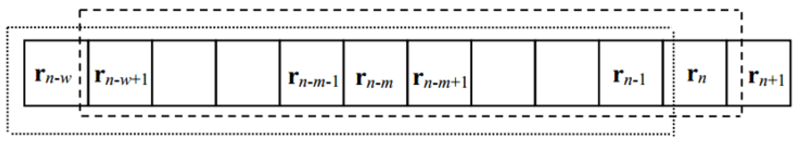
Due to the requirement of causality, local real-time processing would be rather complicated if the commonly used dual window is used. This is because, each time, more than one vector in the local window alters to make sure that the background data sample vectors in the causal sliding window only include the same data sample vectors as before. To address this issue, the literature [16] proposes a local causal sliding array window obtained from stretching out the causal matrix window. The local causal sliding array window of width $w$ slides along with the data sample vector ${\mathbf{r}}_n$ being processed, which performs first in and first out. Figure 1 shows the local causal sliding array window at ${\mathbf{r}}_n$ depicted by dotted lines and the local causal sliding array window at ${\mathbf{r}}_{n+1}$ depicted by dashed lines, where the farthest data sample vector ${\mathbf{r}}_{n-w}$ from ${\mathbf{r}}_n$ in the local causal sliding array window at ${\mathbf{r}}_n$ is removed from the local causal array window at ${\mathbf{r}}_{n+1}$, while the most recent data sample vector ${\mathbf{r}}_n$ is then added to the local causal sliding array window at ${\mathbf{r}}_{n+1}$.

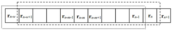
Figure 1. Local causal sliding array windows at ${\mathbf{r}}_n$ and ${\mathbf{r}}_{n+1}$.

2.2.2. Local Causal KRX Detector

By using the local causal sliding array window to get background data sample vectors, the LKRXD can be designed as a local causal KRX detector (LC-KRXD):

$${\delta }^{\mathrm{LC}-\mathrm{KRXD}}\left(\mathsf{\Phi }\left({\mathbf{r}}_n\right)\right)=\hspace{0.17em}{\left({\mathbf{k}}_{\mathbf{r}}^T(n)-k_{\widehat{\mathsf{\mu }}}^T(n)\right)}^T{K}_w^{-1}(n)\left(k_{\mathbf{r}}^T(n)-k_{\widehat{\mathsf{\mu }}}^T(n)\right)$$

(9)

where ${\mathbf{r}}_n$ is the $n^{th}$ sample vector currently being processed, and $K_w(n)$ is called the causal Gram matrix, which is defined by $K_w(n)=k({\mathbf{X}}_w(n),{\mathbf{X}}_w(n))$ where ${\mathbf{X}}_w(n)$ consists of all data sample vectors included in the local causal sliding array window.

In Equation (9), $k_{\mathbf{r}}^T(n)$ and $k_{\widehat{\mathsf{\mu }}}^T(n)$ should meet causality as well. Accordingly, they are represented by

$${\mathbf{k}}_{\mathbf{r}}^T(n)=k({\mathbf{r}}_n,{\mathbf{X}}_w(n))-(\frac{1}{N_w}{\displaystyle \sum _{i=1}^{N_w}k({\mathbf{r}}_n,{\mathbf{x}}_i)}){\mathbf{1}}_{1\times N_w}$$

(10)

$${\mathbf{k}}_{\widehat{\mathsf{\mu }}}^T(n)=(\frac{1}{N_w}{\displaystyle \sum _{i=1}^{N_w}k({\mathbf{x}}_i,{\mathbf{X}}_w(n))})-(\frac{1}{N_w{}^2}{\displaystyle \sum _{i=1}^{N_w}{\displaystyle \sum _{j=1}^{N_w}k({\mathbf{x}}_i,{\mathbf{x}}_j)}}){\mathbf{1}}_{1\times N_w}$$

(11)

where $N_w$ is the total number of data sample vectors in the local causal sliding array window.

2.2.3. Local Real-time KRX Detector

As for LC-KRXD, it is quite time-consuming since every component of Equation (9) has to be recalculated as long as the local causal sliding array window moves. To solve this problem, we develop a local real-time causal KRX detector (LRTC-KRXD) specified by

$${\delta }^{\mathrm{LRTC}-\mathrm{KRXD}}\left(\mathsf{\Phi }\left({\mathbf{r}}_n\right)\right)=\hspace{0.17em}{\left({\mathbf{k}}_{\mathbf{r}}^T(n)-{\mathbf{k}}_{\widehat{\mathsf{\mu }}}^T(n)\right)}^T{K}_w^{-1}(n)\left(k_{\mathbf{r}}^T(n)-k_{\widehat{\mathsf{\mu }}}^T(n)\right)$$

(12)

Employing the Gaussian RBF kernel function denoted by Equation (8), the Gram matrix in the local causal sliding array window at ${\mathbf{r}}_n$ is expressed as

$$K_w\left(n\right)=k\left(X_{n,w},X_{n,w}\right)=\left[\begin{array}{cccc}k({\mathbf{x}}_{n-w},{\mathbf{x}}_{n-w})& k({\mathbf{x}}_{n-w},{\mathbf{x}}_{n-w+1})& \cdots & k({\mathbf{x}}_{n-w},{\mathbf{x}}_{n-1})\\ k({\mathbf{x}}_{n-w+1},{\mathbf{x}}_{n-w})& k({\mathbf{x}}_{n-w+1},{\mathbf{x}}_{n-w+1})& \cdots & k({\mathbf{x}}_{n-w+1},{\mathbf{x}}_{n-1})\\ ⋮& ⋮& & ⋮\\ k({\mathbf{x}}_{n-1},{\mathbf{x}}_{n-w})& k({\mathbf{x}}_{n-1},{\mathbf{x}}_{n-w+1})& \cdots & k({\mathbf{x}}_{n-1},{\mathbf{x}}_{n-1})\end{array}\right]=\left[\begin{array}{ll}{\gamma }_n& {\mathsf{\eta }}_n\\ {\mathsf{\eta }}_n^T& K_n\end{array}\right]$$

(13)

where $X_{n,w}$ is represented by $({\mathbf{x}}_{n-w},{\mathbf{x}}_{n-w+1},\cdots {\mathbf{x}}_{n-1})$ that involves all of the data sample vectors in the local causal sliding array window at ${\mathbf{r}}_n$, ${\gamma }_n$ is given by ${\gamma }_n=k({\mathbf{x}}_{n-w},{\mathbf{x}}_{n-w})$, and ${\mathsf{\eta }}_n$ is a vector obtained by ${\mathsf{\eta }}_n=\left[k({\mathbf{x}}_{n-w},{\mathbf{x}}_{n-w+1}),k({\mathbf{x}}_{n-w},{\mathbf{x}}_{n-w+2}),\cdots ,k({\mathbf{x}}_{n-w},{\mathbf{x}}_{n-1})\right]$. Similarly, the Gram matrix in the local causal sliding array window at ${\mathbf{r}}_{n+1}$ is written as

$$K_w\left(n+1\right)=k\left(X_{n+1,w},X_{n+1,w}\right)=\left[\begin{array}{cccc}k({\mathbf{x}}_{n-w+1},{\mathbf{x}}_{n-w+1})& k({\mathbf{x}}_{n-w+1},{\mathbf{x}}_{n-w+2})& \cdots & k({\mathbf{x}}_{n-w+1},{\mathbf{x}}_n)\\ k({\mathbf{x}}_{n-w+2},{\mathbf{x}}_{n-w+1})& k({\mathbf{x}}_{n-w+2},{\mathbf{x}}_{n-w+2})& \cdots & k({\mathbf{x}}_{n-w+2},{\mathbf{x}}_n)\\ ⋮& ⋮& & ⋮\\ k({\mathbf{x}}_n,{\mathbf{x}}_{n-w+1})& k({\mathbf{x}}_n,{\mathbf{x}}_{n-w+2})& \cdots & k({\mathbf{x}}_n,{\mathbf{x}}_n)\end{array}\right]=\left[\begin{array}{l}{K}_n\hspace{1em}{\mathsf{\beta }}_n^T\\ \hspace{0.17em}{\mathsf{\beta }}_n\hspace{1em}{\chi }_n\end{array}\right]$$

(14)

where $X_{n+1,w}$ is represented by $({\mathbf{x}}_{n-w+1},{\mathbf{x}}_{n-w+2},\cdots {\mathbf{x}}_n)$ involving all of the data sample vectors in the local causal sliding array window at ${\mathbf{r}}_{n+1}$, ${\chi }_n$ is denoted by ${\chi }_n=k({\mathbf{x}}_n,{\mathbf{x}}_n)$, and ${\mathsf{\beta }}_n$ is a vector derived from ${\mathsf{\beta }}_n=\left[k({\mathbf{x}}_n,{\mathbf{x}}_{n-w+1}),k({\mathbf{x}}_n,{\mathbf{x}}_{n-w+2}),\cdots ,k({\mathbf{x}}_n,{\mathbf{x}}_{n-1})\right]$.

The matrix inversion lemma [28,29] is a favored technique to simplify the matrix inversion process and is expressed by

$$R_{m+1}^{-1}={\left[\begin{array}{l}{R}_m\hspace{1em}{\mathbf{U}}_m\\ {\mathbf{V}}_m\hspace{1em}{\mathbf{P}}_m\end{array}\right]}^{-1}=\left[\begin{array}{cc}{R}_m^{-1}+R_m^{-1}{\mathbf{U}}_m{({\mathbf{P}}_m-{\mathbf{V}}_m{R}_m^{-1}{\mathbf{U}}_m)}^{-1}{\mathbf{V}}_m{R}_m^{-1}& -R_m^{-1}{\mathbf{U}}_m{({\mathbf{P}}_m-{\mathbf{V}}_m{R}_m^{-1}{\mathbf{U}}_m)}^{-1}\\ -{({\mathbf{P}}_m-{\mathbf{V}}_m{R}_m^{-1}{\mathbf{U}}_m)}^{-1}{\mathbf{V}}_m{R}_m^{-1}& {({\mathbf{P}}_m-{\mathbf{V}}_m{R}_m^{-1}{\mathbf{U}}_m)}^{-1}\end{array}\right]$$

(15)

${\gamma }_n$ in Equation (13) can be regarded as a 1 × 1 matrix. So if we let ${\gamma }_n=R_m$, ${\mathsf{\eta }}_n^T={\mathbf{V}}_m$, ${\mathsf{\eta }}_n={\mathbf{U}}_m$ and $K_n={\mathbf{P}}_m$, then $K_w^{-1}\left(n\right)$ can be denoted as

$$K_w^{-1}\left(n\right)={\left[\begin{array}{ll}{\gamma }_n& {\mathsf{\eta }}_n\\ {\mathsf{\eta }}_n^T& K_n\end{array}\right]}^{-1}=\left[\begin{array}{cc}{\gamma }_n^{-1}+{\gamma }_n^{-1}{\mathsf{\eta }}_n{(K_n-{\mathsf{\eta }}_n^T{\gamma }_n^{-1}{\mathsf{\eta }}_n)}^{-1}{\mathsf{\eta }}_n^T{\gamma }_n^{-1}& -{\gamma }_n^{-1}{\mathsf{\eta }}_n{(K_n-{\mathsf{\eta }}_n^T{\gamma }_n^{-1}{\mathsf{\eta }}_n)}^{-1}\\ -{(K_n-{\mathsf{\eta }}_n^T{\gamma }_n^{-1}{\mathsf{\eta }}_n)}^{-1}{\mathsf{\eta }}_n^T{\gamma }_n^{-1}& {(K_n-{\mathsf{\eta }}_n^T{\gamma }_n^{-1}{\mathsf{\eta }}_n)}^{-1}\end{array}\right]$$

(16)

Next, we would like to speed up the calculation of $K_w^{-1}$ by deriving the recursive formula between $K_w^{-1}\left(n\right)$ and $K_w^{-1}\left(n+1\right)$, which is one of the main contributions in this paper. Let

$$K_w^{-1}\left(n\right)=\left[\begin{array}{l}a\hspace{1em}\hspace{0.17em}\hspace{0.17em}\hspace{0.17em}\mathbf{b}\\ {\mathbf{b}}^T\hspace{1em}\mathbf{D}\end{array}\right]$$

(17)

According to Equations (16) and (17), we have

$${(K_n-{\mathsf{\eta }}_n^T{\gamma }_n^{-1}{\mathsf{\eta }}_n)}^{-1}=\mathbf{D}$$

(18)

$$K_n^{-1}={({\mathbf{D}}^{-1}+{\gamma }_n^{-1}{\mathsf{\eta }}_n^T{\mathsf{\eta }}_n)}^{-1}$$

(19)

In order to efficiently calculate $K_n^{-1}$ from the known $\mathbf{D}$ and avoid an inverse operation, we use the Woodbury matrix identity [30,31] given by

$${(\mathbf{O}+\mathbf{y}{\mathbf{z}}^T)}^{-1}={\mathbf{O}}^{-1}-\frac{{\mathbf{O}}^{-1}\mathbf{y}{\mathbf{z}}^T{\mathbf{O}}^{-1}}{1+{\mathbf{z}}^T{\mathbf{O}}^{-1}\mathbf{y}}$$

(20)

By virtue of Equation (20), if we also let ${\mathbf{D}}^{-1}=\mathbf{O}$, ${\gamma }_n^{-1}{\mathsf{\eta }}_n^T=\mathbf{y}$, and ${\mathsf{\eta }}_n={\mathbf{z}}^T$, then $K_n^{-1}$ can be transformed into

$$K_n^{-1}=\mathbf{D}-\frac{{\gamma }_n^{-1}\mathbf{D}{\mathsf{\eta }}_n^T{\mathsf{\eta }}_n\mathbf{D}}{1+{\gamma }_n^{-1}{\mathsf{\eta }}_n\mathbf{D}{\mathsf{\eta }}_n^T}$$

(21)

We employ Equation (20) again to derive $K_w^{-1}\left(n+1\right)$. ${\chi }_n$ in Equation (14) can also be treated as a 1 × 1 matrix. Let $K_n=R_m$, ${\mathsf{\beta }}_n={\mathbf{V}}_m$, ${\mathsf{\beta }}_n^T={\mathbf{U}}_m$, and ${\chi }_n={\mathbf{P}}_m$, then $K_w^{-1}\left(n+1\right)$ is finally written as

$${\mathbf{K}}_w^{-1}(n+1)={\left[\begin{array}{l}{K}_n\hspace{1em}{\mathsf{\beta }}_n^T\\ \hspace{0.17em}{\mathsf{\beta }}_n\hspace{1em}{\chi }_n\end{array}\right]}^{-1}=\left[\begin{array}{cc}{K}_n^{-1}+K_n^{-1}{\mathsf{\beta }}_n^T{({\chi }_n-{\mathsf{\beta }}_n{K}_n^{-1}{\mathsf{\beta }}_n^T)}^{-1}{\mathsf{\beta }}_n{K}_n^{-1}& -K_n^{-1}{\mathsf{\beta }}_n^T{({\chi }_n-{\mathsf{\beta }}_n{K}_n^{-1}{\mathsf{\beta }}_n^T)}^{-1}\\ -{({\chi }_n-{\mathsf{\beta }}_n{K}_n^{-1}{\mathsf{\beta }}_n^T)}^{-1}{\mathsf{\beta }}_n{K}_n^{-1}& {({\chi }_n-{\mathsf{\beta }}_n{K}_n^{-1}{\mathsf{\beta }}_n^T)}^{-1}\end{array}\right]$$

(22)

Since ${\chi }_n-{\mathsf{\beta }}_n{K}_n^{-1}{\mathsf{\beta }}_n^T$ is a constant, there is no inverse operation of the matrix existing in Equation (22).

The proposed fast formula for updating $K_w^{-1}\left(n+1\right)$ from $K_w^{-1}\left(n\right)$ consists of the following steps:

Step 1 Obtain $\mathbf{D}$ from ${\mathbf{K}}_w^{-1}(n)$:

$\mathbf{D}={\mathbf{K}}_w^{-1}(\mathrm{n})(2:w,2:w)$

Step 2 Derive $K_n^{-1}$ by $\mathbf{D}$:

$K_n^{-1}=\mathbf{D}-\frac{{\gamma }_n^{-1}\mathbf{D}{\mathsf{\eta }}_n^T{\mathsf{\eta }}_n\mathbf{D}}{1+{\gamma }_n^{-1}{\mathsf{\eta }}_n\mathbf{D}{\mathsf{\eta }}_n^T}$

Step 3 Update $K_w^{-1}\left(n+1\right)$ through $K_n^{-1}$:

${\mathbf{K}}_w^{-1}(n+1)={\left[\begin{array}{l}{K}_n\hspace{1em}{\mathsf{\beta }}_n^T\\ \hspace{0.17em}{\mathsf{\beta }}_n\hspace{1em}{\chi }_n\end{array}\right]}^{-1}=\left[\begin{array}{cc}{K}_n^{-1}+K_n^{-1}{\mathsf{\beta }}_n^T{({\chi }_n-{\mathsf{\beta }}_n{K}_n^{-1}{\mathsf{\beta }}_n^T)}^{-1}{\mathsf{\beta }}_n{K}_n^{-1}& -K_n^{-1}{\mathsf{\beta }}_n^T{({\chi }_n-{\mathsf{\beta }}_n{K}_n^{-1}{\mathsf{\beta }}_n^T)}^{-1}\\ -{({\chi }_n-{\mathsf{\beta }}_n{K}_n^{-1}{\mathsf{\beta }}_n^T)}^{-1}{\mathsf{\beta }}_n{K}_n^{-1}& {({\chi }_n-{\mathsf{\beta }}_n{K}_n^{-1}{\mathsf{\beta }}_n^T)}^{-1}\end{array}\right]$

To save computing time further, ${\mathbf{k}}_{\widehat{\mathsf{\mu }}}^T(n+1)$ can be recursively updated

$${\mathbf{k}}_{\widehat{\mathsf{\mu }}}^T(n)=(\frac{1}{w}{\displaystyle \sum _{i=n-w}^{n-1}k({\mathbf{x}}_i,{\mathbf{X}}_{n,w})})-(\frac{1}{w^2}{\displaystyle \sum _{i=n-w}^{n-1}{\displaystyle \sum _{j=n-w}^{n-1}k({\mathbf{x}}_i,{\mathbf{x}}_j)}}){\mathbf{1}}_{1\times n}={\mathbf{k}}_{m1}(n)-k_{m2}(n){\mathbf{1}}_{1\times n}$$

(23)

$${\mathbf{k}}_{\widehat{\mathsf{\mu }}}^T(n+1)=(\frac{1}{w}{\displaystyle \sum _{i=n-w+1}^{n}k({\mathbf{x}}_i,{\mathbf{X}}_{n+1,w})}-(\frac{1}{w^2}{\displaystyle \sum _{i=n-w+1}^n{\displaystyle \sum _{j=n-w+1}^{n}k({\mathbf{x}}_i,{\mathbf{x}}_j)}}){\mathbf{1}}_{1\times n}={\mathbf{k}}_{m1}(n+1)-k_{m2}(n+1){\mathbf{1}}_{1\times n}$$

(24)

$${\mathbf{k}}_{m1}(n)=\frac{1}{w}{\displaystyle \sum _{i=n-w}^{n-1}k({\mathbf{x}}_i,{\mathbf{X}}_{n,w})}=\left[\frac{1}{w}{\displaystyle \sum _{i=n-w}^{n-1}k({\mathbf{x}}_i,{\mathbf{x}}_{n-w})},\hspace{1em}\frac{1}{w}{\displaystyle \sum _{i=n-w}^{n-1}k({\mathbf{x}}_i,{\mathbf{X}}_{n,2:w})}\right]=\left[\frac{1}{w}({\displaystyle \sum _{i=n-w}^{n-1}{\eta }_{i,n-w}}+\gamma ),\hspace{1em}{\mathbf{k}}_{mf}\right]$$

(25)

$$\begin{array}{ll}{\mathbf{k}}_{m1}(n+1)& =\frac{1}{w}{\displaystyle \sum _{i=n-w+1}^{n}k({\mathbf{x}}_i,{\mathbf{X}}_{n+1,w})}=\left[\frac{1}{w}{\displaystyle \sum _{i=n-w+1}^{n}k({\mathbf{x}}_i,{\mathbf{X}}_{n+1,1:w-1})},\hspace{1em}\frac{1}{w}{\displaystyle \sum _{i=n-w+1}^{n}k({\mathbf{x}}_i,{\mathbf{x}}_n)}\right]\\ & =\left[\frac{1}{w}(w{\mathbf{k}}_{mf}-\mathsf{\eta }+\mathsf{\beta }),\hspace{1em}\frac{1}{w}({\displaystyle \sum _{i=n-w+1}^{n-1}{\beta }_{i,n+1}}+\chi )\right]\end{array}$$

(26)

$$\begin{array}{ll}{k}_{m2}(n+1)& =\frac{1}{w^2}{\displaystyle \sum _{i=n-w+1}^n{\displaystyle \sum _{j=n-w+1}^{n}k({\mathbf{x}}_i,{\mathbf{x}}_j)}}=\frac{1}{w^2}{\displaystyle \sum _{i=n-w}^{n-1}{\displaystyle \sum _{j=n-w}^{n-1}k({\mathbf{x}}_i,{\mathbf{x}}_j)}}-\frac{1}{w^2}{\displaystyle \sum _{j=n-w}^{n-1}k({\mathbf{x}}_{n-w},{\mathbf{x}}_j)}\\ & -\frac{1}{w^2}{\displaystyle \sum _{i=n-w}^{n-1}k({\mathbf{x}}_i,{\mathbf{x}}_{n-w})}+\frac{1}{w^2}{\displaystyle \sum _{j=n-w+1}^{n}k({\mathbf{x}}_n,{\mathbf{x}}_j)}+\frac{1}{w^2}{\displaystyle \sum _{i=n-w+1}^{n}k({\mathbf{x}}_i,{\mathbf{x}}_n)}+k({\mathbf{x}}_{n-w},{\mathbf{x}}_{n-w})-k({\mathbf{x}}_n,{\mathbf{x}}_n)\\ & =\frac{1}{w^2}(w^2{k}_{m2}(n)-2{\displaystyle \sum _{i=n-w}^{n-1}{\eta }_{i,n-w}+}2{\displaystyle \sum _{i=n-w+1}^n{\beta }_{i,n}+\gamma -\chi })\end{array}$$

(27)

where ${\mathbf{X}}_{n,2:w}$ denotes the data sample matrix with the vectors ranging from $2^{th}$ to $w^{th}$ in the local causal sliding array window at ${\mathbf{r}}_n$, and ${\mathbf{X}}_{n+1,1:w-1}$ denotes the data sample matrix with the vectors ranging from $1^{th}$ to ${(w-1)}^{th}$ in the local causal sliding array window at ${\mathbf{r}}_{n+1}$. According to ${\mathbf{k}}_{m1}(n)$, we can obtain ${\mathbf{k}}_{mf}$, and further, ${\mathbf{k}}_{m1}(n+1)$ can be derived by Equation (26). Using Equation (27), $k_{m2}(n+1)$ can be updated by $k_{m2}(n)$. After obtaining ${\mathbf{k}}_{m1}(n+1)$ and $k_{m2}(n+1)$, ${\mathbf{k}}_{\widehat{\mathsf{\mu }}}^T(n+1)$ can be updated recursively by Equation (24).

This paper is inspired by the real-time RX algorithm in the literature [15,16], but it should be noted that both algorithms are different in terms of the original algorithms used to design real-time frames and the processing styles. The real-time RX algorithm is developed based on the RX algorithm, while the proposed algorithm is derived according to the nonlinear version of the RX algorithm, which is more complicated but has a higher detection accuracy. In the recursive process of the real-time RX algorithm, Woodbury matrix identity is used to directly update the inverse covariance matrix. In contrast, the accelerated processing of the proposed algorithm is intricate. The matrix inversion lemma must be associated with the Woodbury matrix identity, in this case, $K_n^{-1}$ can be derived through $\mathbf{D}$. After that, by using the matrix inversion lemma again, $K_w^{-1}\left(n+1\right)$ is finally updated from $K_n^{-1}$. Moreover, the estimated mean of the background data in the kernel space is also recursive in this paper.

3. Description of Hyperspectral Datasets

3.1. Pavia University Dataset

The Pavia University (PaviaU) data were obtained from the Reflective Optics System Imaging Spectrometer (ROSIS) sensor during a flight over Pavia University, northern Italy. They consist of 115 bands ranging from 430 to 860 nm with a 4 nm spectral resolution. The space resolution is approximately 1.3 m. The dataset contains 610 × 340 pixels in the image scene shown in Figure 2. In this study, a subarea shown in Figure 3a was segmented from the initial larger image to conduct experiments. The subset contains 260 × 110 pixels and 103 bands after removing low signal-to-noise ratio (SNR) bands. The ground-truth map is displayed in Figure 3b. Its detailed parameters are presented in Table 1.

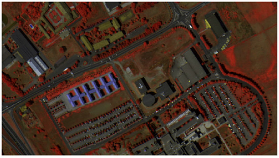
Figure 2. Pavia University hyperspectral image scene.

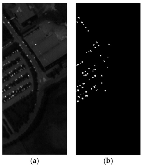
Figure 3. (a) The smaller image scene; (b) ground truth of the smaller image scene.

Table 1. Parameters of the Pavia University hyperspectral dataset. ROSIS is the Reflective Optics System Imaging Spectrometer.

Sensor	ROSIS
Image size	260 × 110
Gray range	0–8000
Wavelength	0.43–0.86 μm
Spectral resolution	4 nm
Spatial resolution	1.3 m
Available bands	103
Location	Pavia University

3.2. Pavia Center Dataset

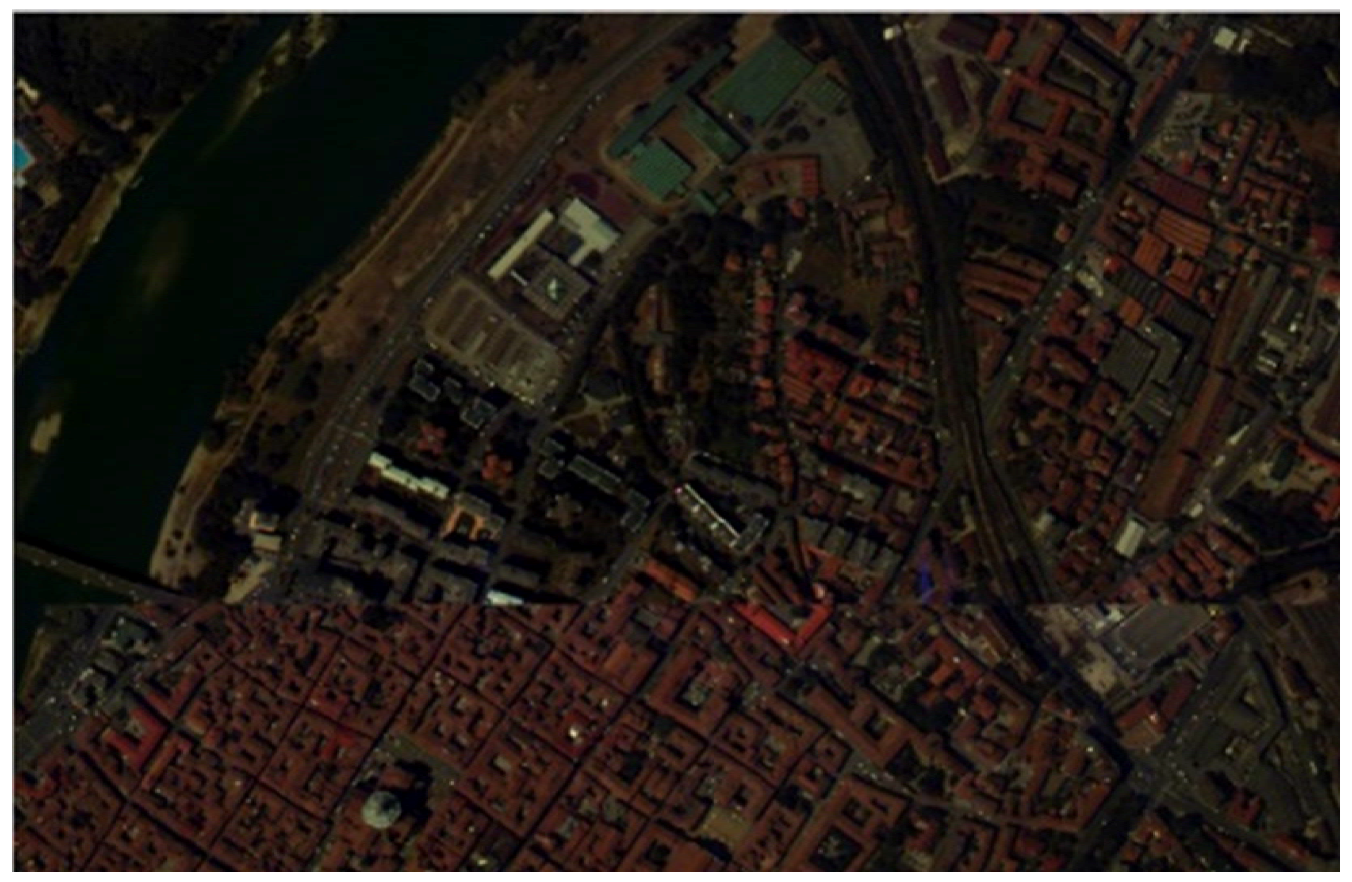
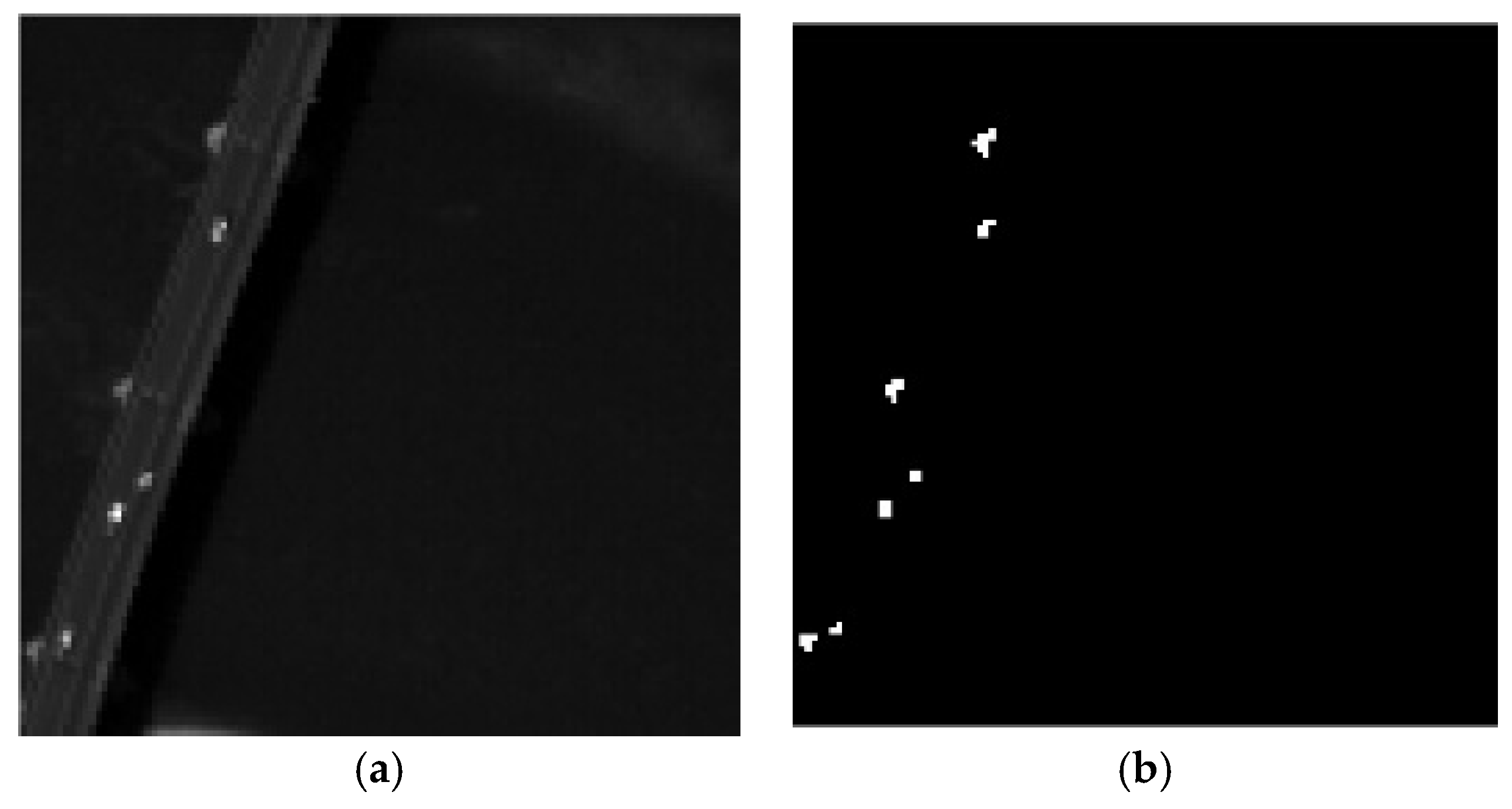
The Pavia Center hyperspectral dataset, acquired by the ROSIS sensor, covers the Pavia Center in northern Italy shown in Figure 4. It is a 115-band image with a size of 1096 × 715 pixels, but only 102 bands were used for experiments after removing low signal-to-noise ratio bands. In this experiment, a smaller subset with a size of 115 × 115 pixels, shown in Figure 5a, was segmented from the initial larger image. Its parameters are presented in Table 2. The smaller image constitutes the background, including a bridge, water and shadows, and anomalies representing vehicles on the bridge, which are shown in Figure 5b.

Figure 4. Pavia Center hyperspectral image scene.

Figure 5. (a) The smaller image scene; (b) ground truth of the smaller image scene.

Table 2. Parameters of the Pavia Center hyperspectral dataset.

Sensor	ROSIS
Image size	115 × 115
Gray range	0–8000
Wavelength	0.43–0.86 μm
Spectral resolution	4 nm
Spatial resolution	1.3 m
Available bands	102
Location	Pavia Center

3.3. San Diego Airport Dataset

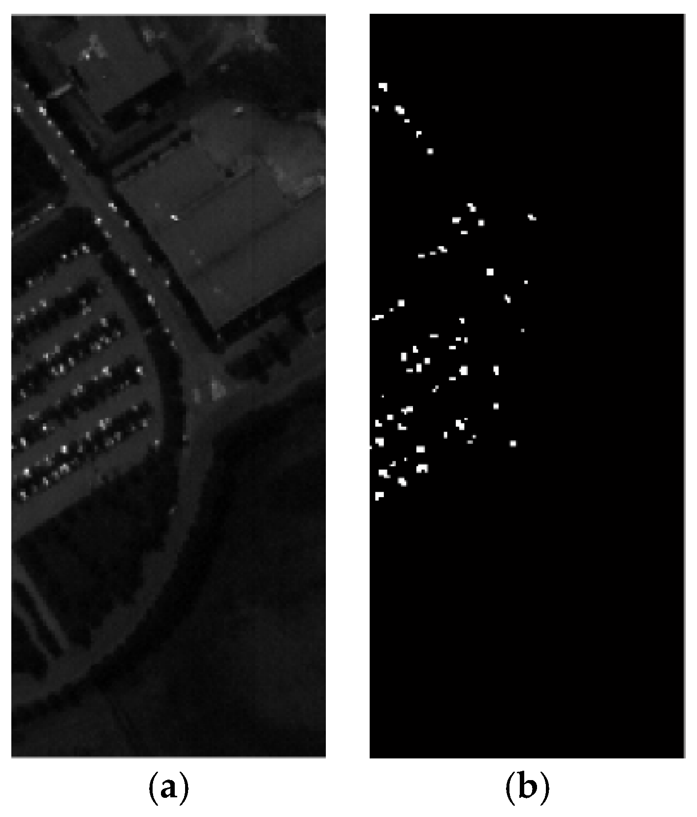
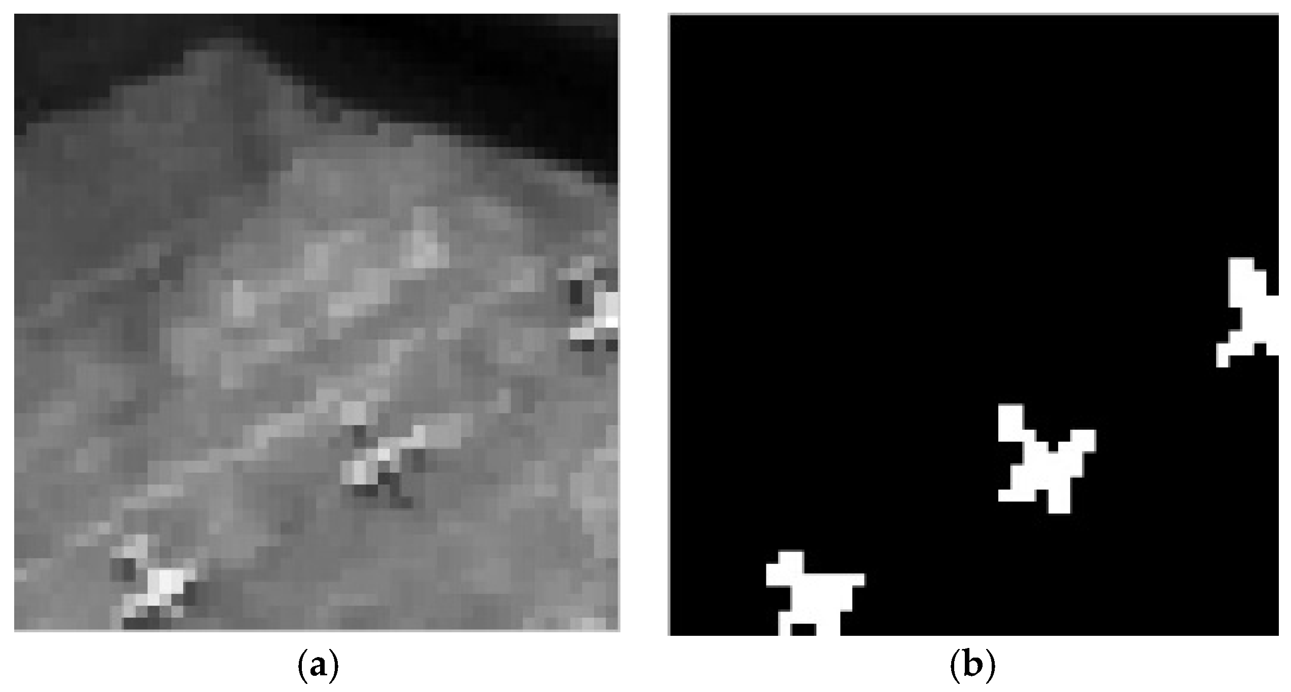
The San Diego Airport dataset was collected by the Airborne Visible/Infrared Imaging Spectrometer (AVIRIS) hyperspectral spectrometer over the area of the San Diego airport and the image is shown in Figure 6. It contains 400 × 400 pixels and 224 bands, 126 of which were used for experiments. A smaller dataset shown in Figure 7a was segmented from the larger image, and its ground truth is given by Figure 7b. Table 3 presents the parameters of the smaller dataset.

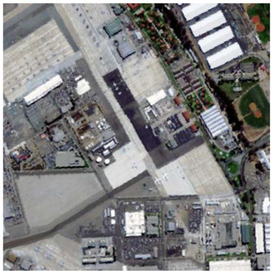
Figure 6. San Diego Airport hyperspectral image scene.

Figure 7. (a) The smaller image scene; (b) ground truth of the smaller image scene.

Table 3. Parameters of the San Diego Airport hyperspectral dataset. AVIRIS is the Airborne Visible/Infrared Imaging Spectrometer.

Sensor	AVIRIS
Image size	51 × 50
Gray range	0–10000
Wavelength	0.4–1.8 μm
Spectral resolution	10 nm
Spatial resolution	3.5 m
Available bands	126
Location	San Diego Airport

4. Experimental Results

In this section, three sets of real hyperspectral datasets, collected by different imaging sensors, are used to perform experimental evaluation for the proposed algorithm.

4.1. Optimum Kernel Parameter on the LRTC-KRXD

This group of experiments explores the optimum Gaussian radial basis function kernel parameter $c$ on the LRTC-KRXD. In the experiments, by virtue of cross-validation, the local causal sliding window width in the LRTC-KRXD on the PaviaU dataset, Pavia Center dataset, and San Diego Airport dataset is manually set to be 70, 40, and 70, respectively.

The receiver operating characteristics (ROC) curve representing detection probability versus false-alarm rates is a strong technique to present quantitative performance analysis. Area under the ROC curve (AUC) is also used to judge the performance of hyperspectral detection. Figure 8 gives the different AUC of the LRTC-KRXD with changing kernel parameter $c$ for all three hyperspectral images. For the PaviaU dataset, the AUC is the largest when $c$ is equal to 100. For the Pavia Center and San Diego Airport datasets, however, the LRTC-KRXD shows the best AUC when $c$ is up to 10. From Figure 8, the AUC for all three datasets rises rapidly between $c={10}^{-1}$ and $c=1$, then they keep basically smooth until $c={10}^6$, which is followed by a steady drop before $c={10}^7$. Therefore, the kernel parameter $c$ is not sensitive to the LRTC-KRXD in some very long numerical range.

Figure 8. The area under the cure (AUC) of the local real-time causal kernel RX detector (LRTC-KRXD) with the changing kernel parameter $c$ on the Pavia University (PaviaU) dataset, Pavia Center dataset, and San Diego Airport dataset.

4.2. Effects of the Local Causal Sliding Array Window Width on the LRTC-KRXD

This group of experiments investigates the performance sensitivity of the LRTC-KRXD in terms of local causal sliding array window width. In these experiments, the local causal sliding array window width in the LRTC-KRXD on three images is manually set from 10 to 130 with steps of 30. By using cross-validation, the parameter $c$ of the Gaussian radial basis function kernel in LRTC-KRXD is set at 100 on the PaviaU dataset and 10 on both the Pavia Center and San Diego Airport datasets.

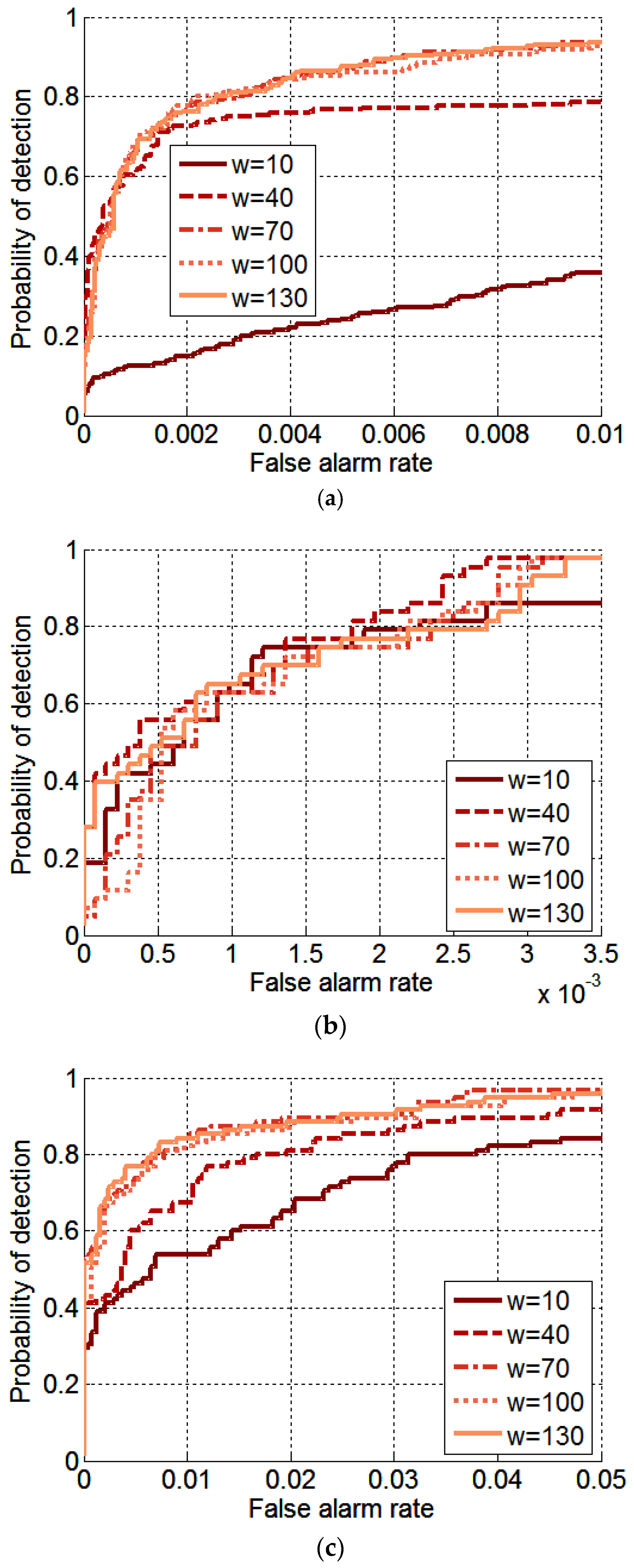
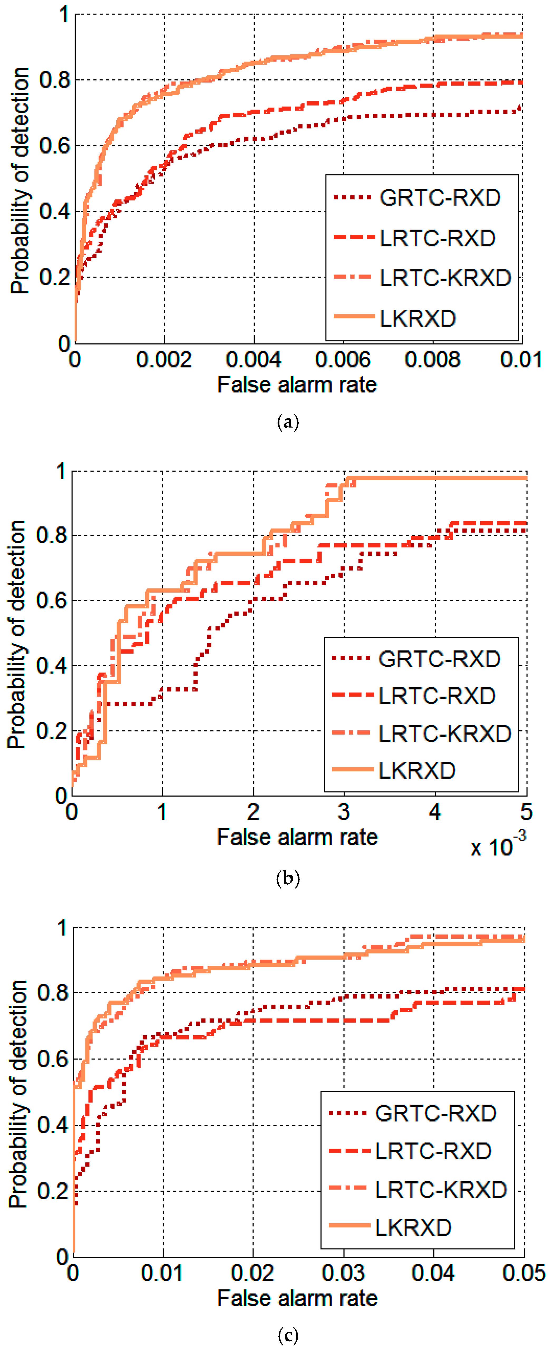
Figure 9 shows the ROC curves of the LRTC-KRXD on three images using changing local causal sliding array window width w between 10 and 130. For the PaviaU dataset in Figure 9a, the detection effect is poor using the local causal sliding array window width w = 10, but the detection performance starts to improve as the local causal sliding window width grows. When it is greater or equal to w = 70, the local causal sliding array window detection performances are comparable. For the Pavia Center dataset in Figure 9b, the ROC curve result with the local causal sliding array window width w = 10 performs the worst, however, the detection accuracy increases when the local causal sliding window width rises. When w = 40, their ROC curves are similar. For the San Diego Airport dataset in Figure 9c, the detection performance improves as the local causal sliding window width w rises from 10 to 70. When it continues to grow, the ROC curve result remains basically unchanged.

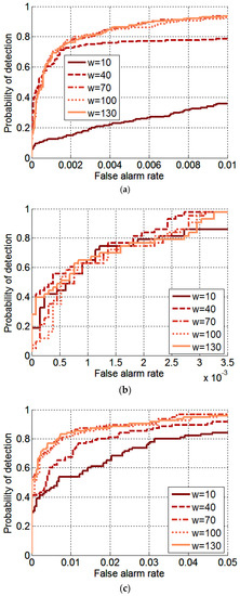
Figure 9. The receiver operating characteristics (ROC) curves of the LRTC-KRXD with changing local causal sliding array window width on the (a) PaviaU dataset; (b) Pavia Center dataset; (c) San Diego Airport dataset.

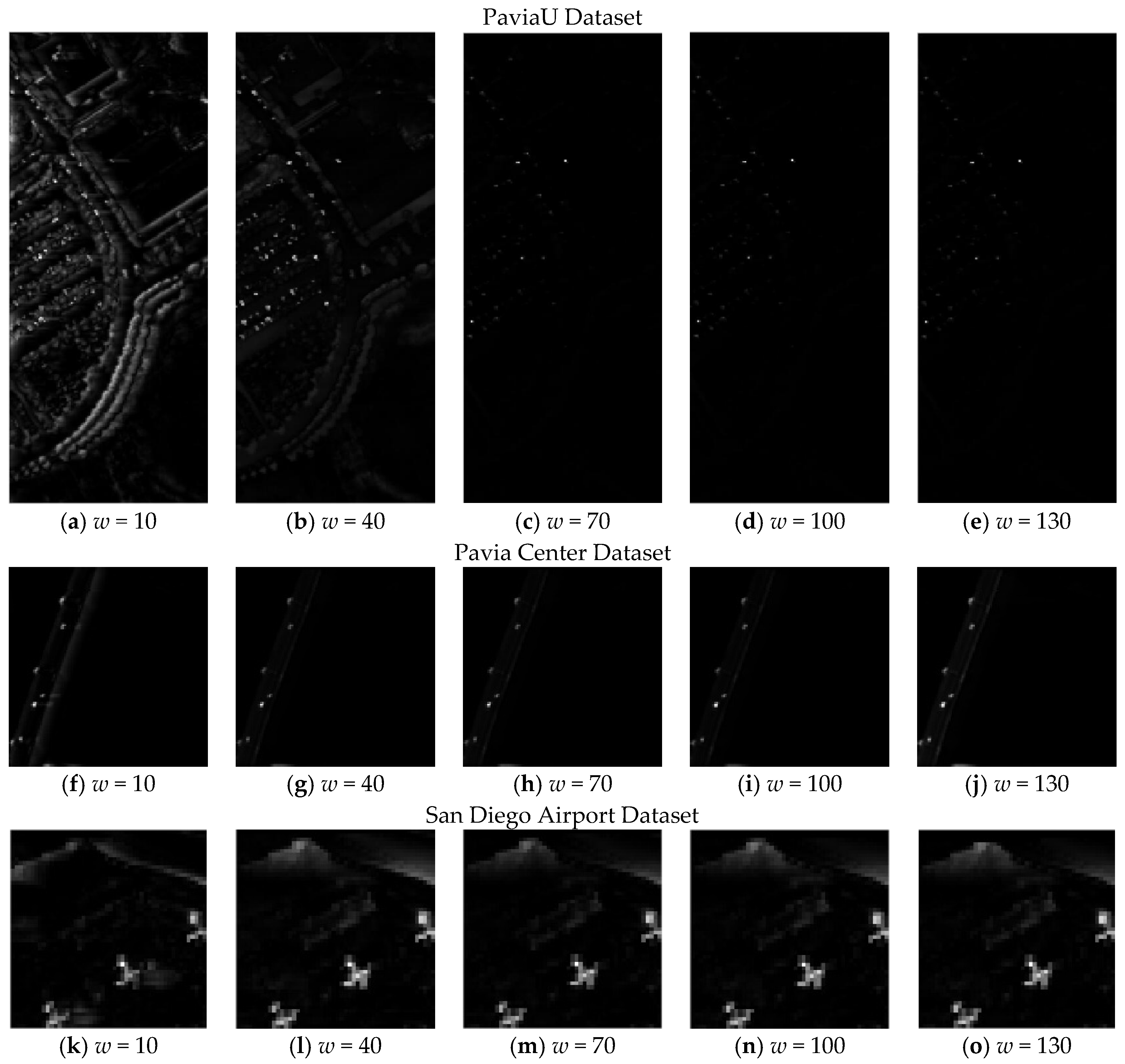
Figure 10 reveals the grayscale results of the above experiments. When the local causal sliding window width w = 10, shown in Figure 10a, f, and k, there is a bad detection effect on the pixels next to the large anomaly in the direction of the window. This is because at those positions, with the small local causal sliding array window width, backgrounds are easily corrupted by the anomalies involved in the local causal sliding array window. As the local causal sliding array window width increases, such phenomena disappear gradually since the number of background pixels in the local causal sliding array window grows. When the local causal sliding array window widths of the LRTC-KRXD on the PaviaU, Pavia Center, and San Diego Airport images are greater or equal to w = 70, w = 40, or w = 70, respectively, their own grayscale outputs are similar by visual inspection.

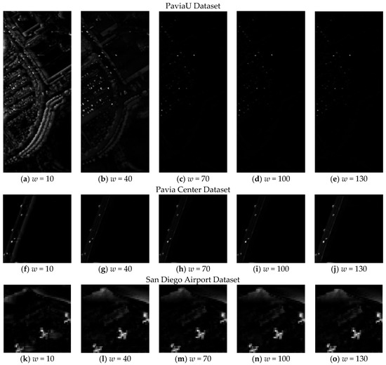
Figure 10. The grayscale results of the LRTC-KRXD with the changing local causal sliding array window width on the PaviaU, Pavia Center, and San Diego Airport datasets.

4.3. Detection Performance of the LRTC-KRXD

These experiments explore the detection performance of the LRTC-KRXD. We made comparisons between the LRTC-KRXD and three other anomaly detectors on three hyperspectral datasets. The other three anomaly detectors included two real-time detectors (GRTC-RXD and LRTC-RXD) and one non-real-time detector (LKRXD). In these experiments, for the LRTC-KRXD, by cross-validation, the parameter $c$ of Gaussian radial basis function kernel is set to 100 on the PaviaU dataset and to 10 on both the Pavia Center dataset and the San Diego Airport dataset. The local causal sliding array window width, w, on the PaviaU dataset and San Diego Airport dataset is set to 70, and the local causal sliding array window width, w, on the Pavia Center dataset is set to 40. For the LRTC-RXD, the local causal sliding array window width, w, on the PaviaU, Pavia Center, and San Diego Airport datasets is set to 400, 300, and 300, respectively, to obtain the best, stable outputs. For the LKRXD, by cross-validation, the set of the kernel parameter $c$ is the same as the LRTC-KRXD on all three images, but the size of the inner window and outer window in the LKRXD is set to 5 and 11, respectively.

Figure 11 shows the results of the ROC curves from all three real-time anomaly detectors and one non-real-time anomaly detector on the three HSI datasets. For the PaviaU dataset shown in Figure 11a, the LRTC-KRXD and the LKRXD are similar throughout the curves, and compared to the GRTC-RXD and the LRTC-RXD, they show a much higher detection probability. For the Pavia Center dataset shown in Figure 11b, the ROC curve results of the LRTC-KRXD and the LKRXD are comparable, but they far outperform those of the GRTC-RXD and the LRTC-RXD. For the San Diego Airport dataset, similar detection effects related to the LRTC-KRXD and the LKRXD are shown in Figure 11c, and these detection effects are better than those of the GRTC-RXD and the LRTC-RXD. This result is because the recursion process of the LRTC-KRXD is derived from the LKRXD that mines nonlinear information by a kernel trick, and there is no information leaked out in this process. Some small differences occur between the detection results of the LRTC-KRXD and the LKRXD because the pseudoinverse of the Gram matrix generally needs to be implemented when each pixel is detected in the LKRXD [32], while this is avoided by recursion in the LRTC-KRXD; the local dual window is used in the LKRXD while the local causal sliding array window is used for the LRTC-KRXD.

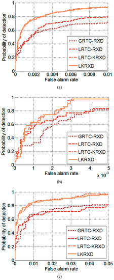
Figure 11. The ROC curves of four anomaly detectors on (a) PaviaU dataset; (b) Pavia Center dataset; (c) San Diego Airport dataset.

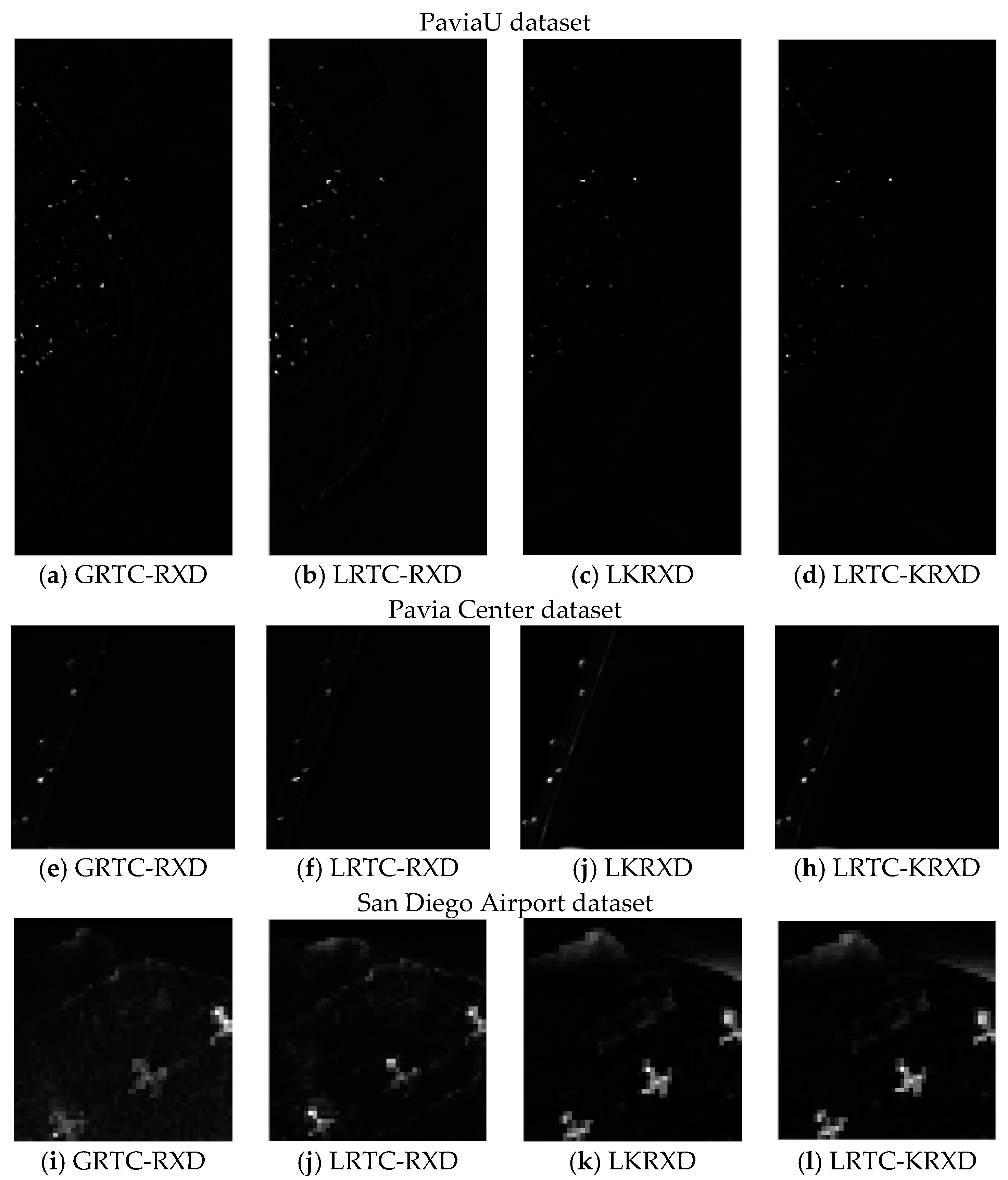
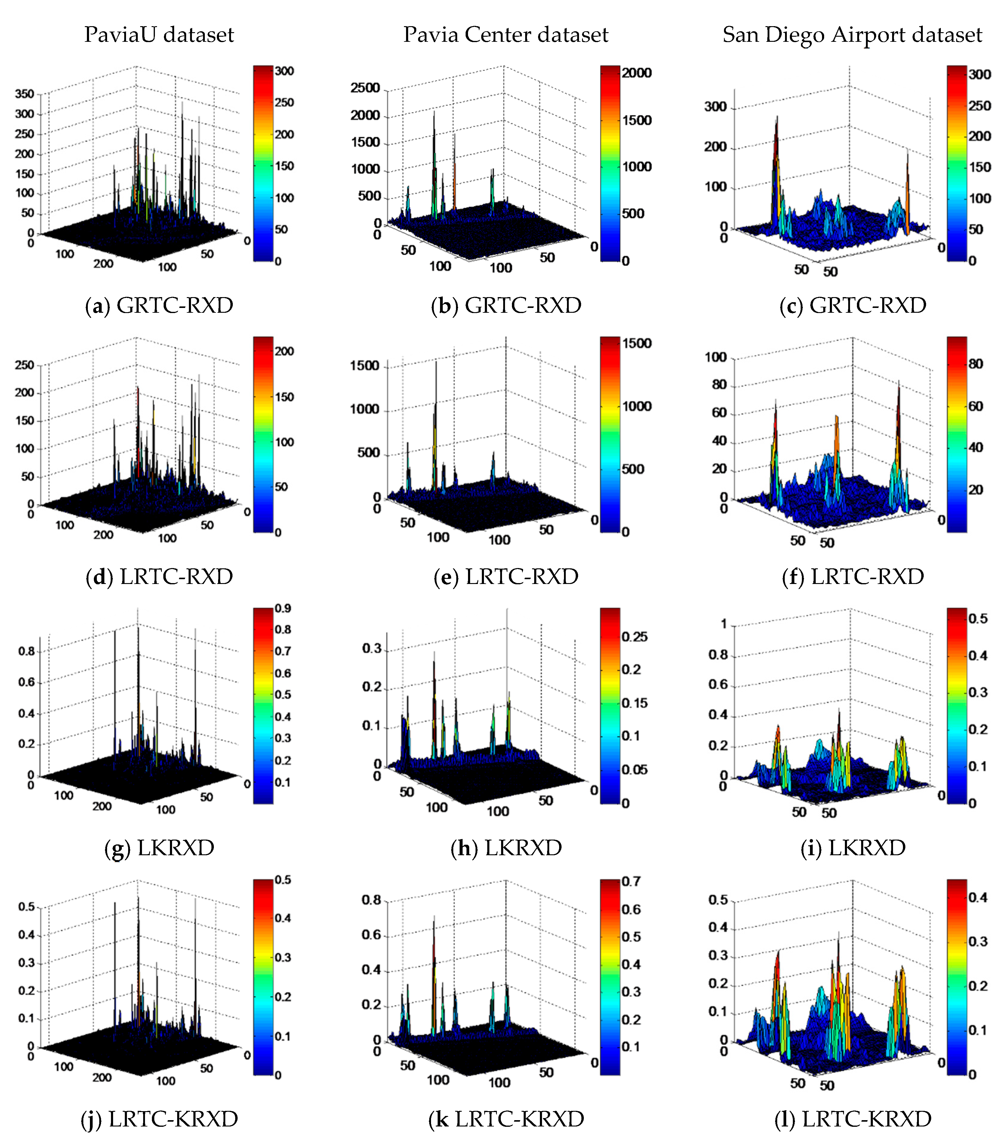
Figure 12 presents the grayscale outputs of ther GRTC-RXD, LRTC-RXD, LKRXD and LRTC-KRXD on three hyperspectral images. For the PaviaU dataset and the Pavia Center dataset, by visual inspection of Figure 12c,d,g,h, there are no appreciable differences, but they clearly show better grayscale results compared with that of Figure 12a,b,e,f. For the San Diego Airport dataset, better background suppression is shown in the LRTC-KRXD and the LKRXD. Three-dimensional (3D) plots are used to verify the detailed differences among the GRTC-RXD, LRTC-RXD, LKRXD, and LRTC-KRXD on the three hyperspectral datasets. As we can see from the 3D plots shown in Figure 13, the detection results of the LKRXD and the LRTC-KRXD are comparable with better detection performances than those of the GRTC-RXD and the LRTC-RXD on both the PaviaU dataset and Pavia Center dataset. It is also clear in Figure 13c,f,i,l that the 3D plots of the LRTC-KRXD and the LKRXD show the robust target clusters.

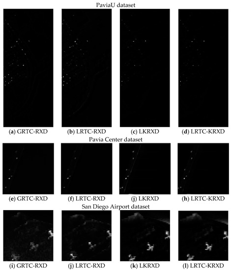
Figure 12. (a–l) The grayscale results of the global real-time causal RX detector (GRTC-RXD), local real-time causal RX detector (LRTC-RXD), local kernel RX detector (LKRXD), and LRTC-KRXD on the PaviaU, Pavia Center, and San Diego Airport datasets.

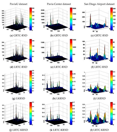
Figure 13. (a–l) The 3D plots of the GRTC-RXD, LRTC-RXD, LKRXD, and LRTC-KRXD on the PaviaU, Pavia Center, and San Diego Airport datasets.

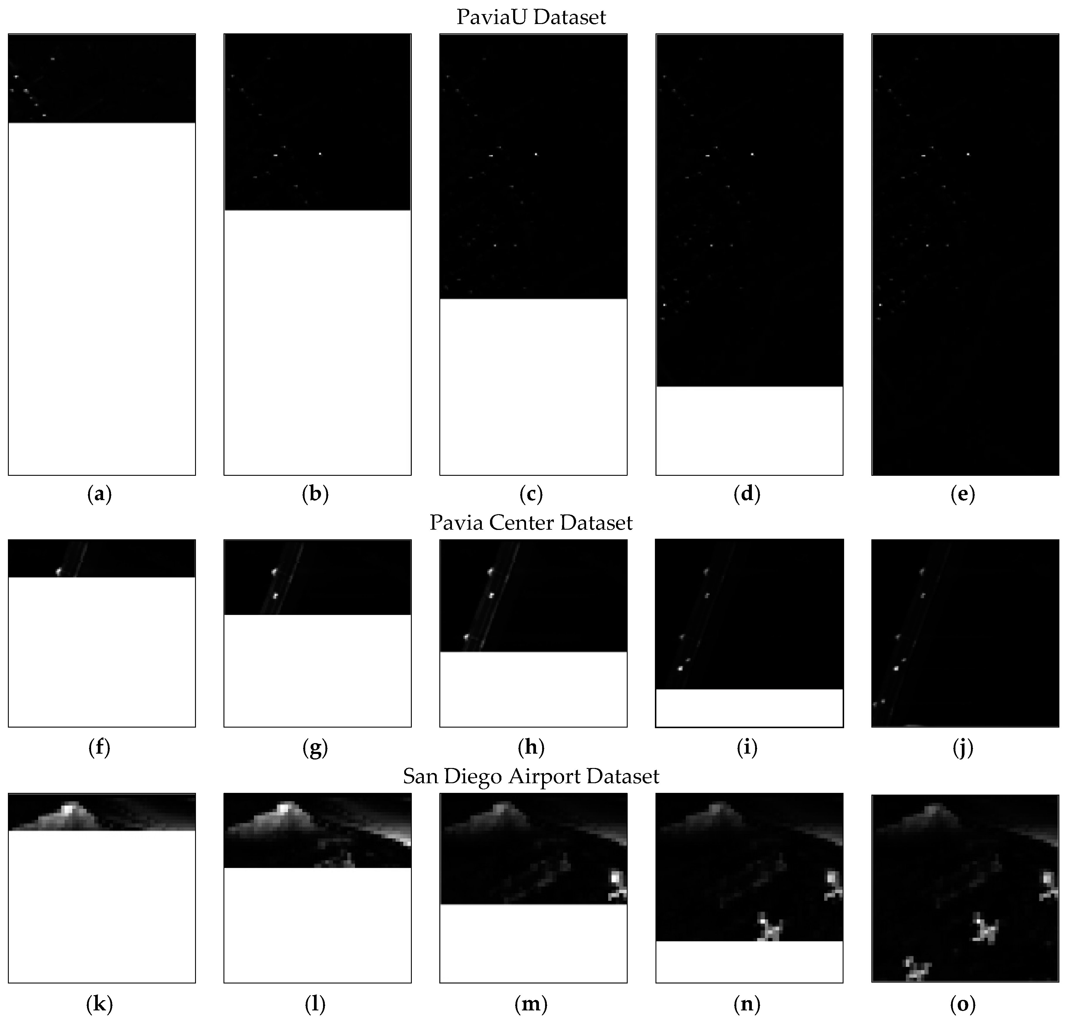
Figure 14 shows the progressive detection procedures of the LRTC-KRXD on the PaviaU, Pavia Center, and San Diego Airport datasets. By using the local causal sliding array window, anomalies in the hyperspectral images are detected pixel-by-pixel in real time. In addition, as time moves along, some weak anomalies appear with various levels of background suppression. For example, on the Pavia Center image, the first three weak anomalies display clearly in the progressive detection results, but when the strong anomaly is detected later, these weak anomalies become dim.

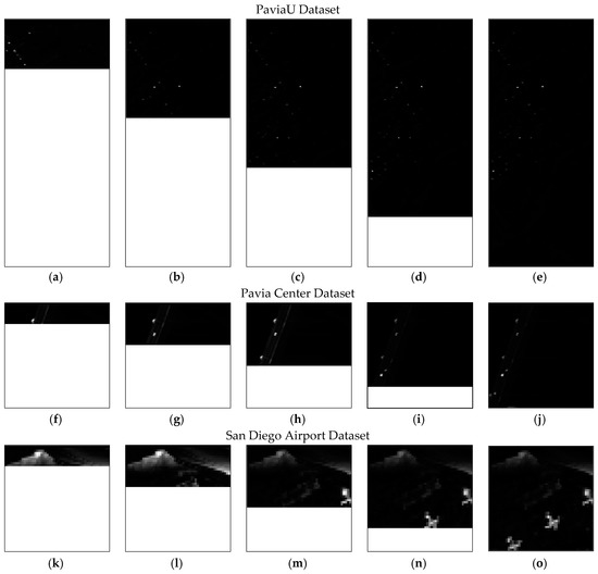
Figure 14. Progressive detection procedures of the LRTC-KRXD on three datasets. (a,f,k) 1/5 detection result; (b,g,l) 2/5 detection result; (c,h,m) 3/5 detection result; (d,i,n) 4/5 detection result; (e,j,o) full detection result.

4.4. Computational Analysis of the LRTC-KRXD

Both computational complexity and computing time are significant indicators to measure the performance of anomaly detection, especially real-time processing. The computational complexity of the LKRX algorithm originates in the components of the LKRX formula specified by Equation (7), including the current pixel in the feature space ${\mathbf{k}}_{\mathbf{r}}^T$, the background data sample mean $k_{\widehat{\mathsf{\mu }}}^T$, the Gram matrix $K_w$ and its inversion $K_w^{-1}$. First, ${\mathbf{k}}_{\mathbf{r}}^T$ is of order $O(\omega \cdot l)$ where ω is the size of the local causal sliding array window and $l$ is the number of bands. It is not really possible to improve it since $\mathbf{r}$ in the equation of ${\mathbf{k}}_{\mathbf{r}}^T$ is not constant when the local sliding array window moves. Second, for $k_{\widehat{\mathsf{\mu }}}^T$, the multiplicative order is approximately $O(\omega )$ without recursive update processing, while using the recursive update equation given by Equation (23), the multiplicative order is close to zero. Third, the multiplicative order of $K_w$ in the LKRXD is $O({\omega }^2\cdot l)+O({\omega }^2\cdot e^m)$ $(m\mathit{\in }R)$, while in the the LRTC-KRX detector, due to the usage of recursive processing, the multiplicative order is not defined (“$n.d.$” entries in Table 4). Lastly, the multiplicative order of $K_w^{-1}$ is reduced to $O({\omega }^2)$ from $O({\omega }^3)$ by virtue of the matrix inversion lemma and Woodbury matrix identity. The more detailed computational complexity is shown in Table 4, where we can see that $O({\omega }^3)$ and $O({\omega }^2\cdot l)$ in the multiplicative order are not involved in LRTC-KRX detection, which reduces much of the computational complexity and cuts down on the massive computing time.

Table 4. Computation complexity of four components.

Computing Components	Multiplicative Order		Additive Order
	LKRXD	LRTC-KRXD	LKRXD	LRTC-KRXD
${\mathbf{k}}_{\mathbf{r}}^T$	$O(\omega \cdot l)$	$O(\omega \cdot l)$	$O(\omega \cdot l)$	$O(\omega \cdot l)$
$k_{\widehat{\mathsf{\mu }}}^T$	$O(\omega )$	0	$O({\omega }^2)$	$O(\omega )$
$K_w$	$O({\omega }^2\cdot l)+O({\omega }^2\cdot e^m)$	$n.d.$	$O({\omega }^2\cdot l)$	$n.d.$
$K_w^{-1}$	$O({\omega }^3)$	$O({\omega }^2)$	$O({\omega }^3)$	$O({\omega }^2)$

The computer environments used for the experiments were 64-bit operating systems with Intel(R) Core (TM) i7-4770K, 3.5 GHz CPU, and 16 GB memory (RAM). All the experiments were conducted five times and averaged to remove computer error [15,16]. Table 5 shows the total computing time of the LKRXD and the LRTC-KRXD on three hyperspectral datasets. By using recursive update equations, the total computing time of the LRTC-KRXD is reduced by at least 44-fold compared to the LKRXD.

Table 5. Processing time for real datasets.

Hyperspectral Data	Total Computing Time (Seconds)		Speedup
	LKRXD	LRTC-KRXD
PaviaU dataset	560.109	11.398	49.141
Pavia Center dataset	247.324	5.030	49.170
San Diego Airport dataset	50.267	1.039	48.380

5. Discussion

In the experiment, the effect of kernel parameter $c$ on the LRTC-KRXD was analyzed. It is clear in Figure 1 that if $c$ is less than 1 or larger than 10⁶ the AUC descends immediately for three datasets. With a wide range (e.g., from 10 to 10⁵) of kernel parameter, the AUC can reach a very high value and basically remain stable. Therefore, it can be concluded that the Gaussian radial basis function kernel parameter $c$ is not sensitive to the LRTC-KRXD in some very long numerical range.

The effect of the local causal sliding window width on real-time detectors was depicted. The results from Figure 9 and Figure 10 indicate that the best detection performance of the LRTC-KRXD is obtained when only a very small local causal sliding window width (less than 100) is utilized. By contrast, the LRTC-RXD needs hundreds of pixels to form the local background information to realize a better detection performance [27]. Due to the requirement of causality, the pixels in the first local causal sliding window are not processed, which implies that the anomalous targets will be missed when they are involved in the initial local causal sliding window. Since the LRTC-KRXD uses fewer pixels than the LRTC-RXD to constitute the local background information, the LRTC-KRXD has a lower probability of missing targets.

In the experiment, the proposed the LRTC-KRXD was also compared with its original algorithm (LKRXD) and two other widely used algorithms (GRTX-RXD and LRTC-RXD). Experimental results on three real data sets illustrate the advantage of the proposed LRTC-KRXD method. The LRTC-KRXD possesses a comparable detection output with the KRXD but higher detection accuracy than the GRTX-RXD and the LRTC-RXD (Figure 11 and Figure 12). For computational complexity and processing time, the results from Table 4 and Table 5 show that the LRTC-KRXD is very computationally efficient. This implies that the LRTC-KRXD achieves a breakthrough in terms of detection accuracy in real-time anomaly detection. Although the LRTC-KRXD gets an over 44-fold speedup, it is sometimes still limited for practical applications. GPU can be taken into account to speed up the processing further using its parallel processing capability.

In the real-time detectors based on the RX algorithm, the size of covariance and the autocorrelation matrix is dependent on the number of bands. So as the number of bands grows, the computational complexity and processing time will increase considerably. For the LRTC-KRXD, however, the Gram matrix is determined by the number of pixels in the local causal sliding window, which means the band growth does not have a great influence on the LRTC-KRXD. This finding can be considered as an encouraging result since modern hyperspectral sensors are characterized by a very high spectral resolution, thus acquiring data on a large number of contiguous bands.

A real-time anomaly detector is implemented pixel-by-pixel, which means that the detection result display of the current pixel is not impacted by subsequent detection results. Accordingly, some weak anomalies detected early may be shown in the detection result (Figure 14). However, this phenomenon cannot appear in non-real-time anomaly detectors that show the final detected anomalies by performing a one-shot operation.

6. Conclusions

Real-time anomaly detection has promising prospective applications and significant practical value. Most real-time anomaly detection algorithms are designed based on the RX detector. However, the real-time RX detector has limitations with the usually undesirable detection output. Therefore, this paper focuses on this issue and develops a new real-time processing framework based on the KRX detector. The kernel RX algorithm has better detection accuracy, but the computation of the Gram matrix and its inverse is computationally inefficient. By taking advantage of the matrix inversion lemma and Woodbury matrix identity, the computation can be recursively updated without repeated calculation. As a result, the kernel RX algorithm complexity is greatly reduced and computing time becomes very short. Our experimental results, conducted using three hyperspectral datasets, indicate that the proposed real-time KRX detector possesses comparable detection accuracy with the original KRX algorithm but with much shorter processing time.

In general, hyperspectral imaging has three data acquisition formats: band interleaved by pixels (BIP) that collects data pixel-by-pixel, band sequential (BSQ) that collects data band-by-band, and band interleaved by lines (BIL) that collects data line-by-line. This paper is designed according to BIP. So both BSQ and BIL can be considered for the real-time KRX implementation in the future. In addition, designing some other computationally efficient methods, for example, using GPU or additional matrix simplification/efficiencies to speed up real-time processing can also be considered for future work.

References

- Wang, Q; Lin, J; Yuan, Y. Salient band selection for hyperspectral image classification via manifold ranking. IEEE Trans. Neural Netw. Learn. Syst. 2016, 27, 1279–1289. [Google Scholar] [CrossRef] [PubMed]
- Chang, C.I. Hyperspectral Imaging: Techniques for Spectral Detection and Classification; Kluwer Academic/Plenum Publishers: New York, NY, USA, 2003. [Google Scholar]
- Chang, C.I. Hyperspectral Data Processing: Algorithm Design and Analysis; Wiley: Hoboken, NJ, USA, 2013. [Google Scholar]
- Reed, I.S.; Yu, X. Adaptive multiple-band CFAR detection of an optical pattern with unknown spectral distribution. IEEE Trans. Signal. Process. 1990, 38, 1760–1770. [Google Scholar] [CrossRef]
- Kwon, H.; Nasrabadi, N.M. Kernel RX-algorithm: A nonlinear anomaly detector for hyperspectral imagery. IEEE Trans. Geosci. Remote Sens. 2005, 43, 388–397. [Google Scholar] [CrossRef]
- Carlotto, M.J. A cluster-based approach for detecting man-made objects and changes in imagery. IEEE Trans. Geosci. Remote Sens. 2005, 43, 374–387. [Google Scholar] [CrossRef]
- Bajorski, P. Practical evaluation of max-type detectors for hyperspectral images. IEEE J. Sel. Top. Appl. Earth Obs. Remote Sens. 2012, 5, 462–469. [Google Scholar] [CrossRef]
- Gurram, P.; Han, T.; Kwon, H. Hyperspectral anomaly detection using sparse kernel-based ensemble learning. Proc. SPIE 2011, 8048, 289–293. [Google Scholar]
- Malpica, J.A.; Rejas, J.G.; Alonso, M.C. A projection pursuit algorithm for anomaly detection in hyperspectral imagery. Pattern Recognit. 2008, 41, 3313–3327. [Google Scholar] [CrossRef]
- Yuan, Y; Ma, D; Wang, Q. Hyperspectral anomaly detection by graph pixel selection. IEEE Trans. Cybern. 2015. [Google Scholar] [CrossRef] [PubMed]
- Ma, L.; Crawford, M.M.; Tian, J. Anomaly detection for hyperspectral images based on robust locally linear embedding. J. Infrared Millim. Terahertz Waves 2010, 31, 753–762. [Google Scholar] [CrossRef]
- Banerjee, A.; Burlina, P.; Diehl, C. A support vector method for anomaly detection in hyperspectral imagery. IEEE Trans. Geosci. Remote Sens. 2006, 44, 2282–2291. [Google Scholar] [CrossRef]
- Schölkopf, B.; Smola, A. Learning with Kernels; MIT Press: Cambridge, MA, USA, 2002. [Google Scholar]
- Stellman, C.M.; Hazel, G.G.; Bucholtz, F.; Michalowicz, J.V.; Stocker, A.; Schaaf, W. Real-time hyperspectral detection and cuing. Opt. Eng. 2000, 39, 1928–1935. [Google Scholar] [CrossRef]
- Chen, S.Y.; Wang, Y.; Wu, C.C.; Liu, C.; Chang, C.I. Real-time causal processing of anomaly detection for hyperspectral imagery. IEEE Trans. Aerosp. Electron. Syst. 2014, 50, 1511–1534. [Google Scholar] [CrossRef]
- Zhao, C.; Wang, Y.; Qi, B.; Wang, J. Global and local real-time anomaly detectors for hyperspectral remote sensing imagery. Remote Sens. 2015, 7, 3966–3985. [Google Scholar] [CrossRef]
- Du, Q.; Nekovei, R. Fast real-time onboard processing of hyperspectral imagery for detection and classification. J. Real Time Image Process. 2009, 4, 273–286. [Google Scholar] [CrossRef]
- Jablonski, J.A.; Bihl, T.J.; Bauer, K.W. Principal component reconstruction error for hyperspectral anomaly detection. IEEE Geosci. Remote Sens. Lett. 2015, 12, 1725–1729. [Google Scholar] [CrossRef]
- Lo, E. Partitioned correlation model for hyperspectral anomaly detection. Opt. Eng. 2015. [Google Scholar] [CrossRef]
- Stevenson, B.; O’Connor, R.; Kendall, W.; Stocker, A.; Schaff, W.; Alexa, D.; Salvador, J.; Eismann, M.; Barnard, K.; Kershenstein, J. Design and performance of the Civil Air Patrol ARCHER hyperspectral processing system. Proc. SPIE 2005. [Google Scholar] [CrossRef]
- Tarabalka, Y.; Haavardsholm, T.V.; Kåsen, I.; Skauli, T. Real-time anomaly detection in hyperspectral images using multivariate normal mixture models and GPU processing. J. Real Time Image Process. 2009, 4, 287–300. [Google Scholar] [CrossRef]
- Molero, J.M.; Garzon, E.M.; Garcia, I.; Quintana-Ortí, E.S.; Plaza, A. Efficient implementation of hyperspectral anomaly detection techniques on GPUs and multicore processors. IEEE J. Sel. Top. Appl. Earth Obs. Remote Sens. 2014, 7, 2256–2266. [Google Scholar] [CrossRef]
- Paz, A.; Plaza, A. GPU implementation of target and anomaly detection algorithms for remotely sensed hyperspectral image analysis. Proc. SPIE 2010. [Google Scholar] [CrossRef]
- Ensafi, E.; Stocker, A.D. An adaptive CFAR algorithm for real-time hyperspectral target detection. Proc. SPIE 2008. [Google Scholar] [CrossRef]
- Acito, N.; Matteoli, S.; Diani, M.; Corsini, G. Complexity-aware algorithm architecture for real-time enhancement of local anomalies in hyperspectral images. J. Real Time Image Process. 2013, 8, 53–86. [Google Scholar] [CrossRef]
- Rossi, A.; Acito, N.; Diani, M.; Corsini, G. RX architectures for real-time anomaly detection in hyperspectral images. J. Real Time Image Process. 2014, 9, 503–517. [Google Scholar] [CrossRef]
- Wang, Y.; Zhao, C.H.; Chang, C.I. Anomaly detection using sliding causal windows. In Proceeding of the 2014 IEEE International Geoscience and Remote Sensing Symposium (IGARSS), Quebec City, QC, Canada, 13–18 July 2014; pp. 4600–4603.
- Bernstein, D.S. Matrix Mathematics; Princeton University Press: Princeton, NJ, USA, 2009. [Google Scholar]
- Higham, N.J. Accuracy and Stability of Numerical Algorithms, 2nd ed.; SIAM: Philadelphia, PA, USA, 2002. [Google Scholar]
- Kay, S. Fundamental of Statistical Signal Processing: Estimation Theory; Prentice Hall: Englewood Cliffs, NJ, USA, 1993. [Google Scholar]
- Kailath, T. Linear Systems; Prentice-Hall: Englewood Cliffs, NJ, USA, 1980. [Google Scholar]
- Theiler, J.; Grosklos, G. Problematic projection to the in-sample subspace for a kernelized anomaly detector. IEEE Geosci. Remote Sens. Lett. 2016, 13, 1–5. [Google Scholar] [CrossRef]
© 2016 by the authors; licensee MDPI, Basel, Switzerland. This article is an open access article distributed under the terms and conditions of the Creative Commons Attribution (CC-BY) license (http://creativecommons.org/licenses/by/4.0/).