Abstract
This study evaluates the quality of the Advanced Spaceborne Thermal Emission Radiometer-Global Digital Elevation Model version 2 (ASTER GDEM2) in comparison with the previous version (GDEM1) as well as the Shuttle Radar Topographic Mission (SRTM) DEM and topographic-map-derived DEM (Topo-DEM) using inundation area analysis for the projected location of the Karian dam, Indonesia. In addition, the vertical accuracy of each DEM is evaluated using the Real-Time Kinematic differential Global Positioning Systems (RTK-dGPS) data obtained from an intensive geodetic survey. The results of the inundation area analysis show that GDEM2 produced a higher maximum contour level (MCL) (64 m) than did GDEM1 (55 m), and thus, GDME2 has a better quality. In addition, the GDEM2-derived MCL is similar to those produced by SRTM DEM (69 m) and Topo-DEM (62 m). The improvement in the contour level in GDEM2 is believed to be related to the successful removal of voids (artifacts) and anomalies present in GDEM1. However, our RTK-dGPS results show that the vertical accuracy of GDEM2 is much lower than that of GDEM1 and the other DEMs, which is contradictory to the accuracy stated in the GDEM2 validation document. The vertical profiles of all DEMs show that GDEM2 contains a comparatively large number of undulation effects, thereby resulting in higher root mean square error (RMSE) values. These undulation effects may have been introduced during the GDEM2 validation process. Although the results of this study may be site-specific, it is important that they be considered for the improvement of the next GDEM version.
1. Introduction
The release of the Advanced Spaceborne Thermal Emission Radiometer-Global Digital Elevation Model version 2 (ASTER GDEM2) has enriched the availability of free-of-charge DEM sources, which are especially useful for developing countries, and prompted users to assess its quality and accuracy. In addition, the GDEM2 version is expected to increase the accuracy of its previous version (GDEM1). In this study, we evaluated the quality of GDEM2 relative to GDEM1, the Shuttle Radar Topographic Mission (SRTM) DEM [1] and a topographic-map-derived DEM (Topo-DEM) using inundation area analysis. The vertical accuracy of each DEM was evaluated using Real-Time Kinematic differential Global Positioning Systems (RTK-dGPS) data collected from a geodetic survey.
Since the initial release in 2003, the SRTM DEM (hereafter called SRTM) has been improved several times, culminating most recently with Version 4. SRTM Version 4, which has a 3 arcsec (approximately 90 m × 90 m) ground resolution, is reported to have a vertical error of less than 16 m at a 90% confidence level [2,3]. In addition, ASTER GDEM data have been improved with the GDEM2 version in October of 2011. It has been reported that the overall accuracy of GDEM2, which has a 30 m ground resolution, is approximately 17 m at a 90% confidence level [4], which is three meters more accurate than GDEM1. Assessments of the accuracy in many different locations throughout the world are critical for improving the next generation of GDEMs.
2. Study Area
To analyze the quality of the newly released GDEM2 in comparison to other DEMs, we focused on the projected location of the Karian dam in the Ciujung watershed, Banten Province, Indonesia. Karian is one of several locations proposed by the local government for the construction of a new dam in the anticipation of population growth and an increased need for water supply by 2025. The coordinates of the dam axis are 106°16′56.10″E; 6°24′45.40″S and 106°17′14.70″E; 6°24′57.50″S.
3. Materials and Methods
3.1. DEM Datasets
GDEM1 and GDEM2 data were obtained from http://asterweb.jpl.nasa.gov [4], and SRTM v4.1 data were acquired from http://srtm.csi.cgiar.org [5]. The Topo-DEM data were derived from digital topographic maps (scale 1:25,000) after being transformed into a DEM using the Triangulated Irregular Network tool in ArcGIS 10 (ESRI, Redlands, CA, USA). The topographic map itself was originally derived from aerial photos (acquired in 1993/1994) using analytical photogrammetric methods, and their accuracy was determined by a field survey by the National Mapping Coordination Agency of Indonesia (the history of the map is written in the legend of the map). The grid size of the Topo-DEM was set to 12.5 m based on both the map accuracy specifications and the scale [6]. Consequently, the grid size of the other DEMs was also resampled to 12.5 m using nearest neighbor interpolation, and the raster pixel type/depth was set to use a 16-bit signed integer format for map algebra operations.
All four of the DEMs (GDEM1, GDEM2, SRTM and Topo-DEM) were referenced to a World Geodetic System (WGS84) horizontal datum and to an Earth Gravitational Model 1996 (EGM96) vertical (geoid) datum. To avoid horizontal offsets, a simple “shifting” method was applied following the method of Hirt et al. [5], where one dataset was systematically shifted by small increments (0.5 arcsec) in all directions and compared against an unshifted dataset. The occurrence of offsets was judged by the root mean square error (RMSE). The results revealed that horizontal offsets did not occur any of the DEMs.
For the purpose of the analysis, we considered Topo-DEM to be the most accurate of the compared DEM datasets because Topo-DEM was produced from high-resolution aerial photos followed by photogrammetry and was verified using a field survey. Therefore, the elevation values contained in the Topo-DEM are actually the bare ground elevations, and thus, this dataset is termed a Digital Terrain Model (DTM). In addition, the elevation values in SRTM and ASTER GDEM constitute the height of the tree canopies and man-made features and thus are termed Digital Surface Models (DSMs) [7].
3.2. Inundation Area Analysis
The basic idea of inundation area analysis is to delineate the impoundment area in a watershed that will be covered by water for a specific purpose, such as for flood and contingency planning analysis [8–10], sedimentation in urban drainages [11], irrigation systems [12] and tsunami run-off areas [13]. Because the main source of information for this analysis is elevation data, inundation area analysis is therefore suitable for evaluating the quality of DEMs. The quality of a DEM itself is mainly dependent on the accuracy of the elevation values, the number of voids (artifacts) and the number of anomalies. In addition to inundation area analysis, other methods are often used for assessing quality of a DEM, including watershed delineation analysis [14] and stream networking analysis [15,16].
In this study, inundation area analysis was applied to determine the maximum contour level (MCL) for the proposed Karian dam. The MCL represents the widest possible inundation area (i.e., the impoundment area) in a watershed that can be covered by water, and the quality of a DEM is evaluated based on the MCL values. The location of the dam axis was used as the basis for the analysis. After applying a fill-and-sink removal procedure [17], all DEM sources were analyzed in ArcGIS 10.
3.3. Vertical Accuracy Assessment
In addition to the inundation area analysis, by which the MCL (impoundment boundary) is evaluated, an assessment of the vertical accuracy of each DEM was also investigated using RTK-dGPS data obtained from a geodetic survey according to a procedure that was previously used in a study in Greece [18]. To examine the accuracy of the DEMs at the watershed scale, the geodetic survey was implemented in several locations of the Ciujung watershed (Figure 1).
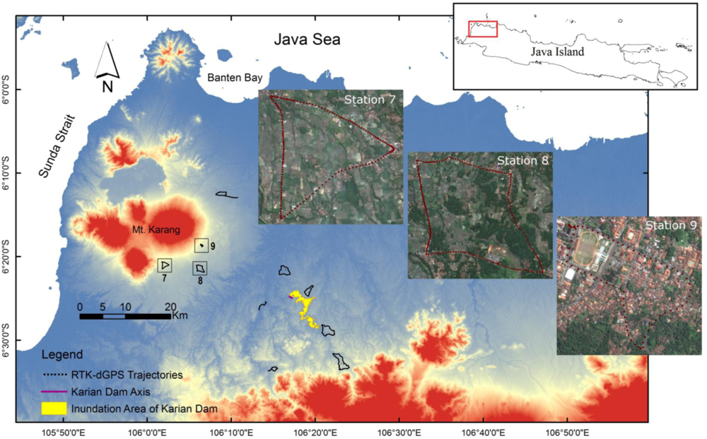
Figure 1.
A map of the study site showing the Real-Time Kinematic differential Global Positioning Systems (RTK-dGPS) trajectories, three of which are enlarged and overlaid on Google Earth images.
Two dGPS Promark3 handsets (Magellan, Smyrna, TN, USA) equipped with 110454-type antennas and 111359-type radio modems were employed during a 3-day field observation study. At each station, the fixed GPS unit was set to a known position (above a national geodetic control point) [19], and the mobile GPS unit, the so-called rover, was used to record the x-y-z positions along a trajectory. An initialization-bar occupation process was required before data collection at each station to resolve the integer ambiguity between the satellites and the rover [20]. Both GPS devices were set to record the positional data at 5-s intervals.
Due to the presence of unpaved roads along certain trajectories, especially in the upstream areas where a car could not travel smoothly at a constant speed, we installed the rover GPS on a motorbike. The use of a motorbike, of course, has an advantage and disadvantage. The advantage was that the motorbike could travel over unpaved roads without difficulty, and the disadvantage was that the motorbike induced a small amount of vibration on the equipment.
The Global Navigation Satellite Systems (GNSS) software version 3.10.11 (Ashtech, Westminster, CO, USA) was used in the post-processing analysis, and we used the RMSE to assess the accuracy due its capacity to encompass both the random and systematic errors in the data [21]. The RMSE has become a standard statistical tool for analyzing DEM accuracy and has been used by the U.S. Geological Survey (USGS) and in many other studies [5,7,18].
4. Results and Discussion
4.1. Inundation Area Analysis
The inundation area analysis applied using the available DEMs produced four impoundment boundaries for the proposed Karian dam. The produced boundaries differ in their MCL, size and volume (Table 1). However, in this study, we only focused on the MCL because the size and volume are secondary products that require a separate investigation.

Table 1.
Maximum contour level, inundation area and water volume derived from various Digital Elevation Models (DEMs) in the projected location of the Karian Dam.
Of the evaluated models, the MCL resulting from GDEM2 was the most similar to the MCL obtained using Topo-DEM, which was considered the most accurate dataset among the comparable DEMs. The MCLs obtained using Topo-DEM and GDEM2 were 62 m and 64 m, respectively. The SRTM data produced a slightly higher MCL of 69 m. In addition, the GDEM1 data yielded the lowest MCL value of only 55 m. The shapes of the impoundment boundaries obtained using GDEM2 and SRTM were highly similar to that of the Topo-DEM. Meanwhile, a small difference in the boundary was observed for GDEM1 (Figure 2).
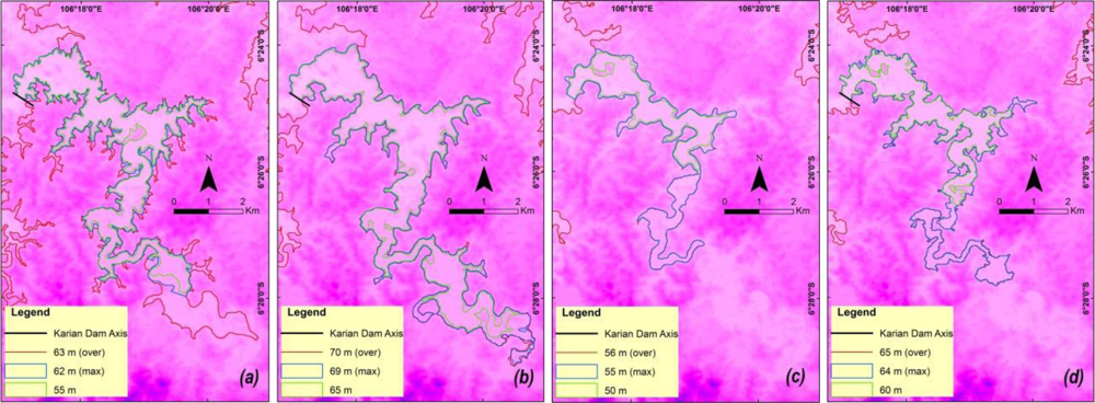
Figure 2.
Contour level of the inundation areas for the proposed location of the Karian dam produced from (a) Topo-DEM; (b) SRTM DEM; (c) ASTER GDEM1; (d) ASTER GDEM2.
The more accurate contouring level of GDEM2 relative to SRTM and GDEM1 demonstrated that GDEM2 has been improved regarding voids, anomalies and flat lake surface problems. These artifacts have been substantially reduced from GDEM1 by the National Geospatial-Intelligence Agency (NGA) using an extensive visual identification method [4]. The remaining difference in the MCL of Topo-DEM and the MCLs of SRTM/GDEM2 could be related to conceptual differences in DTM/DSM. The effect of the canopy and man-made features on the elevation value is an interesting subject for future studies. The factors influencing the large differences in the size and volume of the impoundment boundaries also require further investigation.
Although the observations reported here are based on a simple analysis, the results imply that GDEM1 users should be cautious when using these data, especially when GDEM1 is used for hydrologic studies that require precise results, such as flood disaster analysis. Up to this point, the use of GDEM2 and SRTM is strongly recommended because these datasets provided better impoundment boundaries.
The results of this analysis, however, could not provide information regarding the accuracy of the vertical elevation of the DEMs. Although an MCL is based on elevation values, the created boundary is strongly dependent on the conditions surrounding the dam axis and the projected dam, such as the terrain, slope and land cover. The accuracy of a DEM in a large watershed can only be evaluated by conducting an intensive geodetic survey, in which a huge number of geographic positions (x, y and z) of the earth are densely recorded over a trajectory in several different types of terrain and land cover. After performing a geodetic survey, the vertical profile of each DEM can be compared with the elevation values that were measured in the field.
4.2. Vertical Accuracy Assessment
Although the analysis presented above demonstrated an improvement of GDEM2 over GDEM1, the elevation values of the DEMs must also be assessed. In this section, the vertical accuracy of each DEM is evaluated based on the height values derived from a geodetic RTK-dGPS dataset.
4.2.1. The Quality of RTK-dGPS Data
Within the limitation of the survey design, as described in the Materials and Methods section, the RTK-dGPS data produced satisfactory Positional Dilution of Precision (PDOP) values with an average of 2.26 ± 0.54 (determined from 3,661 survey points); 36.5% of the values were within the range of 1–2, whereas the remaining 63.5% were within the range of 2–5. Based on the work of Kaya and Saritaş [22], the PDOP ranges of 1–2 and 2–5 are classified as “excellent” and “good”, respectively. The number of satellites in view (SV), with an average of 8.21 ± 1.30, was also adequate for typical hydrological studies.
The measures of PDOP and SV are useful for assessing GPS data quality [23,24]. An additional important measure of GPS quality is the estimated accuracy of GPS data. It was difficult to estimate the overall horizontal and vertical accuracies of our data because the rover GPS traveled across different types of land cover. The results showed excellent accuracy when the rover GPS traveled across open roads; however, the accuracy decreased when certain high objects (e.g., trees and man-made features) were present along the roadsides or when the distance between two GPS unit was greater than 1 km.
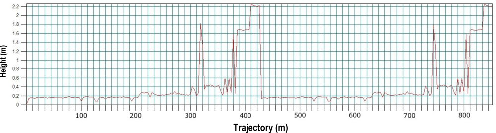
An example of the vertical accuracy assessment is presented using data from Station 6 (Figure 3), where two peaks of biases appeared in the result due to the aforementioned influences. At this station, the estimated horizontal and vertical accuracies were 0.625 m and 0.605 m, respectively, or 0.427 m and 0.402 m, respectively, when the influencing factors are filtered out. The biases from the other stations were higher and dependent on the land cover types along the roads and the distance between the pair of GPS units. Here, we note that the survey design requires certain improvements to eliminate the effects of the land cover types and decrease the distance between the GPS units.

Figure 3.
Estimated vertical accuracy of RTK-dGPS data for Station 6.
4.2.2. Vertical Accuracy of the DEMs
After filtering out the large outliers influenced by high objects, the RTK-dGPS data were used to measure the vertical accuracy of all DEMs compared in this study, including the Topo-DEM. Although the Topo-DEM was considered to have the most accurate data, it may contain certain elevation biases relative to the RTK-dGPS data. The vertical accuracy assessment was applied not only to the DEMs at their original resolutions but also to the DEMs after being resampled to the smallest resolution, which was equal to the 12.5 m resolution of the Topo-DEM.
Our results showed that when comparing the DEMs at their original resolutions, the Topo-DEM demonstrated the most accurate data with an average RMSE of 3.204 m at the 95% confidence level (Table 2). Among the satellite-derived DEMs, the SRTM data showed a better vertical accuracy than both GDEM1 and GDEM2. More surprisingly, the vertical accuracy of GDEM2 was less than the accuracy of GDEM1, as it achieved a much higher RMSE compared to GDEM1. This result was surprising because it was contradictory to the accuracy reported by the GDEM2 validation team [4].
Table 2.
Results of vertical accuracy assessment between various DEMs with Real-Time Kinematic differential Global Positioning Systems (RTK-dGPS) data using a linear regression model.
After resampling to 12.5 m × 12.5 m resolution, the comparison of the accuracy of all DEMs was repeated. The resampling procedure greatly increased the accuracy of all DEMs, as demonstrated by their average RMSEs. Moreover, the vertical accuracy of SRTM was now better than that of Topo-DEM, which indicates that the Topo-DEM data may need certain corrections or revalidation. Nevertheless, this procedure demonstrated that SRTM continued to yield a better accuracy than both GDEM versions, and GDEM2 data yielded the lowest vertical accuracy of all the tested DEM datasets. The greater accuracy of SRTM over GDEM1 has been previously reported in many studies [5,14,25,26]. However, this study is the first investigation to report the lower accuracy of GDEM2 data.
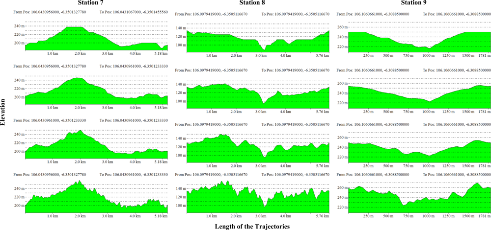
To determine the cause of the relatively low accuracy of GDEM2, we plotted the vertical profiles of the DEMs along the dGPS trajectories. Three examples of these profiles are shown in Figure 4. We chose these trajectories because for these data, the rover travelled along good-quality paved roads. These results demonstrated that the GDEM2 data contain a large extent of undulation effects, thereby causing high RMSE values.

Figure 4.
Vertical profiles of digital elevation data along the RTK-dGPS trajectories as indicated in Figure 1. The sequence of the elevation data from the first row to the last row is Topo-DEM, SRTM DEM, ASTER GDEM1 and ASTER GDEM2.
Given that the rover GPS for these stations was moving along good-quality paved roads, it is impossible that the trajectories reflect a large degree of unevenness of the roads. Instead, we believe that the undulation effects in GDEM2 may have been introduced during the validation process. The GDEM2 validation team has explained that the validation process included cloud effects removal, land cover reclassification, canopy effects reduction, the addition of a number of scenes and other factors [4] through which the undulation effects may have been inadvertently introduced.
4.2.3. Undulation Effects
In addition to the elevation difference in the DTM/DSM, which was previously addressed, it is always important to remember that elevation information contained in a dataset is different depending on the baseline reference. GPS delivers ellipsoidal heights, whereas SRTM and GDEM provide mean sea level (MSL) heights. The difference between these data, which is called the geoid height, varies for any location of in world because the MSL heights are affected by gravitational forces.
We analyzed Station 7 an example of the dataset (Figure 5). In our data, the elevation of the Topo-DEM was mostly (but not in all cases) lower than the SRTM and GDEM because the later datasets contained the bare ground elevation. In addition, the SRTM and GDEM elevations were higher than in the Topo-DEM because they included the canopy height information. At this station, the average geoid heights are 3.835 m, 4.478 m and 5.372 m for SRTM, GDEM1 and GDEM2, respectively. Although disparities between the DEMs are best judged according to their RMSE values [5,7,18], the average geoid heights and the undulation pattern, as displayed in Figure 5, can help in understanding the disparities between datasets.
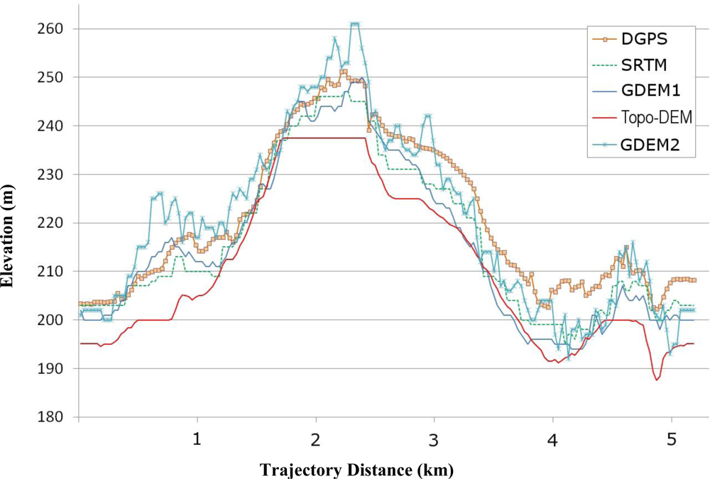
Figure 5.
Height disparities and different undulation levels among the DEMs for Station 7.
5. Conclusions
This study provides additional information for public users and the GDEM2 validation team regarding the quality of GDEM2 data. Inundation area analysis of the projected Karian dam (Indonesia) and the RTK-dGPS data collected from Ciujung watershed were used to assess the quality of GDEM2 data. The results of inundation area analysis showed that the GDEM2 data was highly improved by the removal of voids and anomalies and thereby produced a better MCL (impoundment boundary). The MCL produced from GDEM2 was 64 m, which was a much better value than the MCL produced from GDEM1 (55 m) and closer to the MCL produced from Topo-DEM (62 m) and SRTM-DEM (69 m). However, the vertical accuracy of GDEM2 was found to be lower than that of GDEM1 and the other DEMs, as indicated by the RTK-dGPS data and the RMSE values. The average RMSE values for the Topo-DEM, SRTM, GDEM1 and GDEM2 were 3.204, 3.250, 4.045 and 5.683, respectively. The lower accuracy of GDEM1 could be caused by undulation effects, which were found throughout the observed stations. Although our initial findings cannot be generalized to all GDEM2 data, we are pleased to report that there is evidence of the undulation effects in GDEM2 present in the study area. We believe that the undulation effects may have been introduced during the validation process, perhaps due to cloud effect removal, land cover reclassification or other factors that are unknown to the authors. To obtain a clear understanding of these effects, an intensive study involving additional sampling stations over a wider area is necessary in the future.
Acknowledgments
This study was funded by the Global Environmental Leader (GEL) Project of the Graduate School for International Development and Cooperation (IDEC), Hiroshima University, Japan.
References
- Farr, T.G.; Korbick, M. Shuttle radar topography mission produces a wealth of data. Eos Trans. AGU 2000, 81, 583–585. [Google Scholar]
- Jarvis, A.; Reuter, H.I.; Nelson, A.; Guevara, E. Hole-Filled Seamless SRTM Data V4. Available online: http://srtm.csi.cgiar.org/ (accessed on 14 February 2012).
- Rodríguez, E.; Morris, C.S.; Belz, Z.E. A global assessment of the SRTM performance. Photogramm. Eng. Remote Sensing 2006, 72, 249–260. [Google Scholar]
- ASTER GDEM Validation Team. ASTER Global DEM Validation: Summary of Validation Results. Available online: http://www.ersdac.or.jp (accessed on 9 January 2012).
- Hirt, C.; Filmer, M.S.; Featherstone, W.E. Comparison and validation of the recent freely-available ASTER-GDEM ver1, SRTM ver4.1 and GEODATA DEM-9S ver3 digital elevation models over Australia. Aust. J. Earth Sci 2010, 57, 337–347. [Google Scholar]
- Tobler, W. Resolution, Resampling, and All That. In Building Data Bases for Global Science; Mounsey, H., Tomlinson, R., Eds.; Taylor and Francis: London, UK, 1988; pp. 129–137. [Google Scholar]
- Miliaresis, G.; Delikaraoglou, D. Effects of percent tree canopy density and DEM misregistration on SRTM/DEM vegetation height estimates. Remote Sens 2009, 1, 36–49. [Google Scholar]
- Manfreda, S.; di Leo, M.; Sole, A. Detection of flood prone areas using digital elevation models. J. Hydrol. Eng 2011, 16, 781–790. [Google Scholar]
- Han, K.Y.; Lee, J.T.; Park, J.H. Flood inundation analysis resulting from Levee-break. J. Hydraul. Res 1998, 5, 747–759. [Google Scholar]
- Sippel, S.J.; Hamilton, S.K.; Melack, J.M.; Choudhury, B.J. Determination of inundation area in the Amazon River floodplain using the SMMR 37 GHz polarization difference. Remote Sens. Environ 1994, 48, 70–76. [Google Scholar]
- Moojong, P.; Hwandon, J.; Minchul, S. Estimation of sediments in urban drainage areas and relation analysis between sediments and inundation risk using GIS. Water Sci. Technol 2008, 58, 811–817. [Google Scholar]
- Hagiwara, T.; Kazama, S.; Sawamoto, M. Relationship between inundation area and irrigation area on flood control in the lower Mekong River. Adv. Hydraul. Water Eng 2002, 1–2, 590–595. [Google Scholar]
- McAdoo, B.G.; Richardson, N.; Borrero, J. Inundation distances and run-up measurements from ASTER, QuickBird and SRTM data, Aceh coast, Indonesia. Int. J. Remote Sens 2007, 28, 2961–2975. [Google Scholar]
- Gamett, B.J. An Accuracy Assessment of Digital Elevation Data and Subsequent Hydrologic Delineations in Lower Relief Terrain. Idaho State University, Pocatello, ID, USA, 2010. [Google Scholar]
- Hosseinzadeh, S.R. Drainage network analysis, comparison of digital elevation model (DEM) from ASTER with high resolution satellite image and aerial photographs. Int. J. Environ. Sci. Dev 2011, 2, 194–198. [Google Scholar]
- Hengl, T.; Heuvelink, G.B.M.; van Loon, E.E. On the uncertainty of stream networks derived from elevation data: The error propagation approach. Hydrol. Earth Syst. Sci. Discuss 2010, 7, 767–799. [Google Scholar]
- Lindsay, J.B. The terrain analysis system: A tool for hydro-geomorphic applications. Hydrol. Process 2005, 19, 1123–1130. [Google Scholar]
- Mouratidis, A.; Briole, P.; Katsambalos, K. SRTM 3″ DEM (version 1, 2, 3, 4) validation by means of extensive kinematic GPS measurements: A case study from North Greece. Int. J. Remote Sens 2010, 31, 6205–6222. [Google Scholar]
- Soetadi, J. A Model for a Cadastral Land Information System for Indonesia; University of New South Wales: Sydney, NSW, Australia, 1988. [Google Scholar]
- Magellan Navigation Inc. Promark3/Promark3 RTK Reference Manual; Magellan Navigation Inc: San Dimas, CA, USA, 2005. [Google Scholar]
- Nikolakopoulos, K.G.; Kamaratakis, E.K.; Chrysoulakis, N. SRTM vs. ASTER elevation products: Comparison for two regions in Crete, Greece. Int. J. Remote Sens 2006, 27, 4819–4838. [Google Scholar]
- Kaya, F.A.; Saritaş, M. A Computer Simulation of Dilution of Precision in the Global Positioning System Using Matlab. Proceedings of the 4th International Conference on Electrical and Electronic Engineering, Bursa, Turkey, 7–11 December 2005.
- Kaplan, E.D.; Hegarty, E.J. Understanding GPS: Principles and Applications; Artech House: London, UK, 2005. [Google Scholar]
- Natural Resources Canada. Satellite Visibility and Availability. In GPS Positioning Guide; Natural Resources Canada: Ottawa, ON, Canada, 1995; pp. 15–19. [Google Scholar]
- Pryde, J.K.; Osorio, J.; Wolfe, M.L.; Heatwole, C.; Benham, B.; Cardenas, A. Comparison of Watershed Boundaries Derived from SRTM and ASTER Digital Elevation Datasets and from a Digitized Topographic Map. Proceedings of ASABE Meeting, Minneapolis, MN, USA, 17–20 June 2007.
- Kervyn, M.; Ernst, G.G.J.; Goosens, R.; Jacobs, P. Mapping volcano topography with remote sensing: ASTER vs. SRTM. Int. J. Remote Sens 2008, 29, 6515–6538. [Google Scholar]