AI-Enabled Frequency Diverse Array Spaceborne Surveillance Radar for Space Debris and Threat Detection Under Resource Constraints

Highlights

What are the main findings?

• This paper proposes two matrix-completion-based methods that can effectively suppress the sidelobes in the beamforming results of random FDA radar.
• The proposed method can achieve stable and high-quality beamforming for FDA radar while reducing the hardware cost of its transceiver units, and it does not require large-scale pre-training data.

What are the implications of the main findings?

• This method only uses observed data to accomplish signal processing for random FDA radar, making it suitable for practical engineering applications.
• The improved sidelobe suppression effect enhances the accuracy of beamforming results and provides strong support for various subsequent downstream tasks.

Abstract

Ensuring space environment security through the detection of space debris and non-cooperative threat objects has become a critical mission for next-generation spaceborne surveillance systems. Frequency diversity array (FDA) radar, with its unique range angle-dependent beampattern, offers a transformative capability to distinguish closely-spaced space threats from intense background clutter. However, the operational deployment of spaceborne FDA is inherently hindered by stringent platform resource constraints, including limited power supply, high hardware complexity, and restricted data transmission bandwidth. These physical limitations inevitably lead to incomplete signal observations, resulting in elevated sidelobes that can obscure small, high-speed space debris. To bridge the gap between hardware constraints and high-fidelity surveillance, this paper proposes an AI-enabled data recovery framework based on deep matrix factorization. Specifically designed to process the complex-valued nature of radar echoes, the proposed framework introduces two specialized architectures: a real-valued representation-based method (DMF-Rr) and a native complex-valued deep matrix factorization (CDMF) network that preserves vital phase coherence. By leveraging deep learning to “enable” sparse-sampled systems, the proposed method effectively reconstructs missing observations without requiring prior knowledge of the signal rank. Numerical results demonstrate that the AI-powered CDMF significantly suppresses the high sidelobes induced by resource-limited sampling, enabling the reliable identification and localization of weak threat objects. This study demonstrates the power of AI in overcoming the physical bottlenecks of spaceborne hardware, providing a robust solution for enhancing space situational awareness in an increasingly crowded orbital environment.

1. Introduction

The sustainable use of outer space is increasingly threatened by the rapid proliferation of space debris and the emergence of non-cooperative orbital objects, as illustrated in Figure 1. With the deployment of massive satellite constellations in low earth orbit (LEO) [1,2,3], ensuring space situational awareness (SSA) has become a strategic priority to prevent catastrophic collisions and safeguard spaceborne assets. Among various monitoring sensors, spaceborne surveillance radar stands out as a pivotal tool due to its all-weather, all-day operational capability and its sensitivity to high-speed moving objects. However, detecting and tracking small-scale space debris against complex cosmic backgrounds requires radar systems with unprecedented resolution and interference mitigation capabilities [4,5,6].

To address the challenges of discriminating closely-spaced threats and suppressing range-ambiguous clutter, frequency diversity array (FDA) radar has emerged as a transformative waveform-diverse technique for next-generation spaceborne platforms [7]. Unlike traditional phased-array radars, FDA provides an additional degree of freedom by introducing a frequency increment across the array elements, resulting in a range angle-dependent beampattern [8,9,10]. This unique physical property is essential for spaceborne surveillance, as it enables the radar to distinguish between targets that share the same azimuth but reside at different ranges, which is a common scenario in space debris cloud monitoring.

Despite its theoretical advantages, the practical implementation of FDA on spaceborne platforms encounters a fundamental bottleneck: the severe stringency of onboard resource constraints [11]. Therefore, the random FDA radar has emerged as required [12]. The random FDA radar has also gained much attention because it reduces system cost with affordable performance loss by only receiving randomly selected frequency channels, instead of all the transmission frequencies. However, when conventional beamforming (CBF) is directly performed on random FDA, the missing data (caused by the abandoned frequency channels) may result in high sidelobes, affecting the estimate performance of radar targets [12,13,14].

To suppress the high sidelobes occurring in random FDA, this paper proposes an AI-enabled data recovery framework based on deep matrix factorization [15,16,17]. Moving beyond traditional analytical methods such as matrix factorization (MF) [18,19,20,21,22,23] that require prior knowledge of the matrix rank—a parameter difficult to estimate for unknown space debris—our approach leverages the power of deep learning to “enable” sparse-sampled systems. We specifically address the complex-valued nature of radar signals by introducing a native complex-valued deep matrix factorization (CDMF) network. This architecture preserves vital phase coherence, which is indispensable for precise target localization and interference suppression in waveform-diverse systems. By treating signal reconstruction as an intelligence-driven task, this study demonstrates that AI can effectively compensate for physical hardware limitations, providing a robust solution for ensuring space environment security in increasingly crowded orbital regimes.

The main contributions of this paper are reflected in three aspects: First, we propose modifying the input parameters of deep matrix factorization by changing the low-rank complex-valued matrix to a structurally similar low-rank real matrix. We then use deep matrix factorization to complete this real matrix, indirectly achieving the completion of the original complex-valued matrix. Second, we propose modifying the structures and activation functions of the neural network used in deep matrix factorization to enable complex-valued number computations, allowing for the completion of complex-valued matrices. Finally, simulated results of FDA signal processing demonstrate the effectiveness of the two methods we proposed.

The data used in this article can be queried by contacting the corresponding author. Some of the experimental results in this paper have already been published in IEEE International Conference on Signal, Information and Data Processing 2024. The conference version mainly focused on the proposal of the core idea, methodological framework, and preliminary validation, with only limited and simplified simulation results due to space constraints. In contrast, in this paper, we extend the algorithm to the spaceborne FDA radar system for space debris detection, which is a more practical and challenging scenario. Compared with [24], we conduct more sufficient comparison experiments with a variety of classical and state-of-the-art methods, including matrix completion methods, such as singular value thresholding (SVT) and low-rank matrix fitting (LMaFit), different variants of the proposed algorithm, and other beamforming approaches. The ablation experiments and contrastive results more convincingly demonstrate the superiority of the complex-valued deep matrix factorization method in target localization, mainlobe accuracy, and sidelobe suppression. In this submission, we provide more rigorous and detailed mathematical derivations of the complex-valued deep matrix factorization model, including the loss function construction, optimization process, time complexity analysis, and possible application for space debris and threat detection. The theoretical framework is more systematic and complete than the preliminary version in [24], which enhances the theoretical soundness and readability of the paper.

The rest of the paper is organized as follows. In Section 2, we review the matrix completion problem, matrix factorization, and deep matrix factorization, and we explain the drawbacks of matrix factorization and deep matrix factorization. We then propose two modifications to deep matrix factorization: On one hand, by modifying its input parameters, we indirectly complete a complex-valued matrix. On the other hand, by modifying the neural network’s architecture and activation functions, we enable it to perform complex-valued number calculations. In Section 3, we introduce the signal model and signal processing methods of FDA radar and explain how complex-valued matrix completion can be applied to the processing of random FDA radar signals. Experimental results are presented in Section 4. Discussion and conclusions are finally presented in Section 5 and Section 6.

Notation: The symbol $\mathbb{C}$ represents the set of complex numbers. Correspondingly, ${\mathbb{C}}^M$ and ${\mathbb{C}}^{M\times N}$ are the sets of the M-dimensional vectors and $M\times N$ matrices of complex numbers, respectively. The subscripts ${[·]}_i$ and ${[·]}_{i,k}$ are used for the i-th entry of a vector and the i-th row, k-th column entry of a matrix. We let $[·]$ and $\{·\}$ denote a vector/matrix and a set, respectively. $\overline{·}$ denotes the conjugate operation. The transpose of a vector or a matrix is written as the superscript ${(·)}^T$. ⊙ represents the Hadamard product of two matrices. $rank(·)$ represents the rank of a matrix. ${\parallel ·\parallel }_F$ represents the Frobenius norm of a matrix. We let $\mathrm{Re}\{·\}$ and $\mathrm{Im}\{·\}$ represent taking the real parts and the imaginary parts, respectively.

2. Traditional and Proposed Complex-Valued Matrix Completion Methods

In this section, we introduce traditional matrix completion methods and our proposed methods for the complex-valued matrix completion problem. To this aim, we review the matrix completion problem in Section 2.1, and then we introduce the method of matrix completion using traditional matrix factorization and its shortcomings in Section 2.2. Subsequently, we introduce the method of matrix completion using deep learning in Section 2.3.

2.1. Problem Formulation

Consider a matrix $\mathbf{X}\in {\mathbb{C}}^{N_1\times N_2}$ with rank r, where $r\ll \min \{N_1,N_2\}$. Suppose that we sample the matrix $\mathbf{X}$ on a set $\mathrm{\Omega }$, resulting in

$$S_{\mathrm{\Omega }}\left(\mathbf{X}\right)={\mathbf{H}}_{\mathrm{\Omega }}\odot \mathbf{X},$$

(1)

where ${\mathbf{H}}_{\mathrm{\Omega }}\in {\mathbb{C}}^{N_1\times N_2}$ is a sampling matrix defined by

$$\begin{array}{c}\hfill {\left[{\mathbf{H}}_{\mathrm{\Omega }}\right]}_{i,j}=\left\{\begin{array}{c}1,\mathrm{if}(i,j)\in \mathrm{\Omega },\hfill \\ 0,\mathrm{else}.\hfill \end{array}\right.\end{array}$$

(2)

The matrix completion problem is to recover matrix $\mathbf{X}$ from the undersampled matrix $S_{\mathrm{\Omega }}\left(\mathbf{X}\right)$. Due to the low-rank assumption of $\mathbf{X}$, the matrix completion problem can be expressed as

$$\begin{array}{cc}\hfill & {\displaystyle \underset{\mathbf{M}}{\mathrm{arg\; min}}}rank\left(\mathbf{M}\right),\hfill \\ \hfill & s.t.S_{\mathrm{\Omega }}\left(\mathbf{X}\right)=S_{\mathrm{\Omega }}\left(\mathbf{M}\right),\hfill \end{array}$$

(3)

where $\mathbf{M}\in {\mathbb{C}}^{N_1\times N_2}$. Unfortunately, the rank minimization problem (3) is NP-hard [25]. Therefore, some alternative algorithms including matrix factorization-based methods are proposed, as introduced below.

2.2. Matrix Factorization

Matrix factorization methods usually seek for a low-rank representation of $\mathbf{X}$ by two low-dimensional matrices $\mathbf{P}\in {\mathbb{C}}^{N_1\times r}$ and $\mathbf{Z}\in {\mathbb{C}}^{r\times N_2}$, given by

$$\begin{array}{c}\hfill \mathbf{X}\approx \mathbf{P}\mathbf{Z}.\end{array}$$

(4)

These matrices are found by solving the following optimization problem:

$$\begin{array}{cc}\hfill & {\displaystyle \underset{\mathbf{P},\mathbf{Z},\mathbf{M}}{\mathrm{arg\; min}}}{\parallel \mathbf{M}-\mathbf{P}\mathbf{Z}\parallel }_F^2,\hfill \\ \hfill & s.t.S_{\mathrm{\Omega }}\left(\mathbf{X}\right)=S_{\mathrm{\Omega }}\left(\mathbf{M}\right).\hfill \end{array}$$

(5)

where $\mathbf{M}\in {\mathbb{C}}^{N_1\times N_2}$. To address Problem (5), Wen et al. proposed the Gauss–Seidel-based LMaFit algorithm [18], and Jain et al. proposed the gradient descent-based Alternating minimization for matrix completion (AltMinComplete) algorithm [23]. These matrix factorization methods have low computational burden and show good recovery performance when the rank r is exactly given. However, such prior knowledge is not available in many applications, where these matrix factorization methods suffer from significant performance loss. This inspires the development of deep matrix factorization-based methods, and some more sophisticated algorithms are proposed, introduced subsequently.

2.3. Deep Matrix Factorization

In this subsection, we introduce the method of matrix completion by applying deep learning to matrix factorization: deep matrix factorization [15]. These deep learning methods generally rely on some off-the-shelf deep learning toolboxes like TensorFlow 2.16.1 and PyTorch 2.2.2, which, however, are designed for real-valued networks [26] and are not applicable for complex-valued matrix completion. Therefore, we need methods that allow neural networks to perform complex-valued operations. In this subsection, we introduce how to modify the input parameters, or structures and activation functions of a standard real-valued neural network, to enable it to handle complex-valued calculations. In Section 2.3.1, we present the methods of using deep learning for real matrix completion and how to revise them in complex-valued matrix completion problems. Then, in Section 2.3.2, we propose two methods to improve previous deep matrix factorization for the complex-valued matrix completion problem.

2.3.1. For Real-Valued Matrices

Unlike traditional matrix factorization, the deep matrix factorization-based method does not require prior knowledge on the rank of matrix; hence, it is expected to outperform traditional matrix factorization methods. For a matrix $\mathbf{A}\in {\mathbb{R}}^{N_1\times N_2}$, the deep matrix factorization method approximates $\mathbf{A}$ as $\mathbf{A}\approx \mathbf{U}\mathbf{V}$ by generating $\mathbf{U}\in {\mathbb{R}}^{N_1\times r^{\prime }}$ and $\mathbf{V}\in {\mathbb{R}}^{r^{\prime }\times N_2}$ using neural networks [15]. In this approach, the parameter $r^{\prime }$ is not required to be equal to the rank of $\mathbf{A}$, denoted as $r=\mathrm{rank}\left(\mathbf{A}\right)$, which distinguishes it from traditional matrix factorization methods.

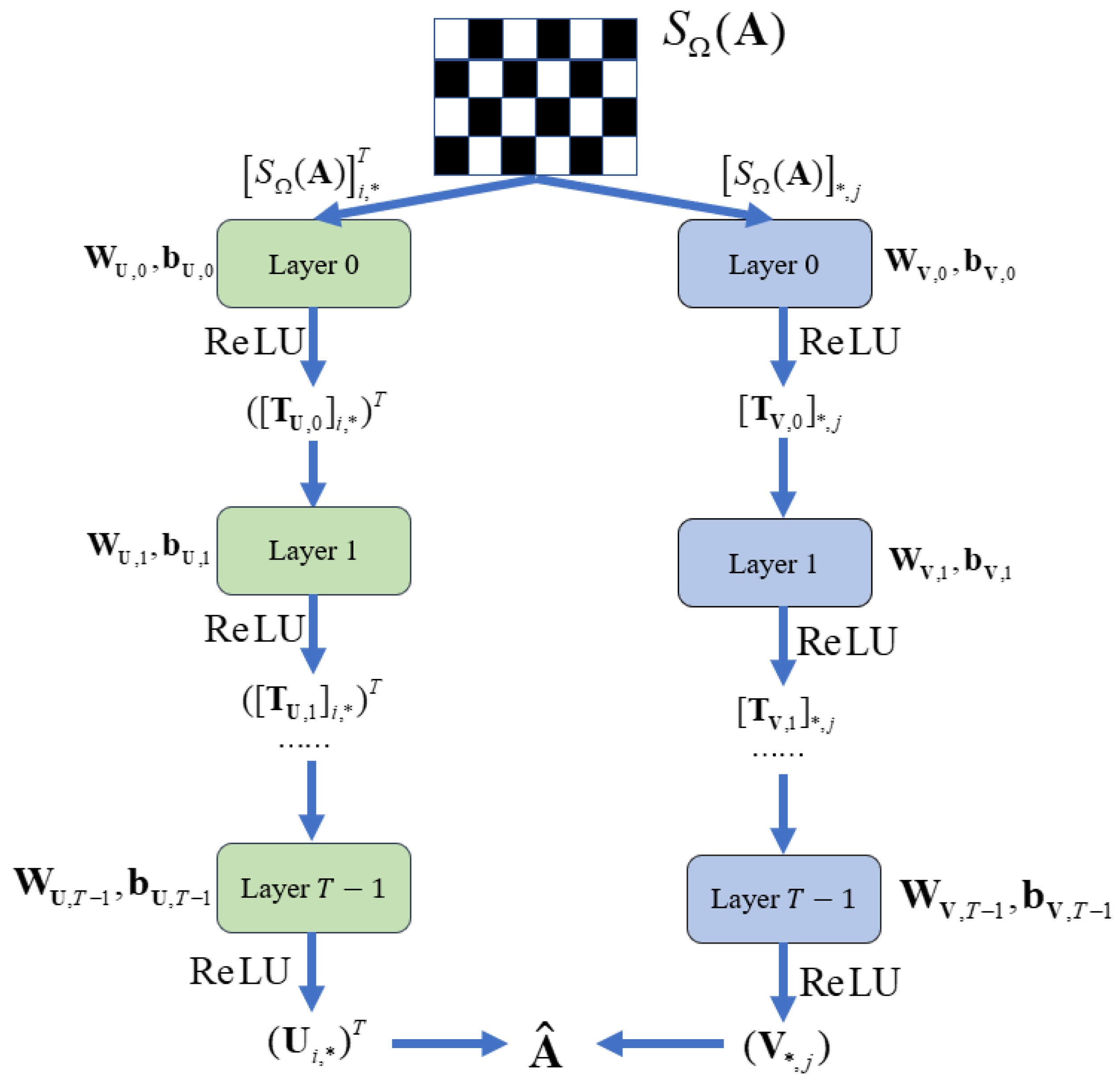
We then review the deep matrix factorization method, of which the architecture is illustrated in Figure 2. It applies two neural networks to generate $\mathbf{U}$ and $\mathbf{V}$, shown on the left and right sides of the figure, respectively. Both neural networks have similar structure, but the inputs and outputs are different: When inputing the transpose of a row of the sampled matrix $S_{\mathrm{\Omega }}\left(\mathbf{A}\right)$, the left neural network outputs the transpose of the corresponding row of $\mathbf{U}$; instead, inputing a column of $S_{\mathrm{\Omega }}\left(\mathbf{A}\right)$ yields the corresponding column of $\mathbf{V}$.

Both neural networks consist of T layers, each employing a fully connected structure. As an example, we consider how to generate $\mathbf{U}$, i.e., the left part of Figure 2. We then provide the details of the l-th hidden layer for generating $\mathbf{U}$. With the input vector ${\left({\left[{\mathbf{T}}_{\mathbf{U},l-1}\right]}_{i,\ast }\right)}^T\in {\mathbb{R}}^{M_{l-1}}$, where the index ∗ denotes all the elements and $\mathbf{U}$ in the subscript indicates that the neural network is design for generating $\mathbf{U}$, this layer outputs the vector ${\left({\left[{\mathbf{T}}_{\mathbf{U},l}\right]}_{i,\ast }\right)}^T\in {\mathbb{R}}^{M_l}$ as follows:

$${\left({\left[{\mathbf{T}}_{\mathbf{U},l}\right]}_{i,\ast }\right)}^T=f({\mathbf{W}}_{\mathbf{U},l}{\left({\left[{\mathbf{T}}_{\mathbf{U},l-1}\right]}_{i,\ast }\right)}^T+{\mathbf{b}}_{\mathbf{U},l}),$$

(6)

where $M_{l-1}$ is the input dimension, $M_l$ is the output dimension, ${\mathbf{W}}_{\mathbf{U},l}\in {\mathbb{R}}^{M_l\times M_{l-1}}$ is called the weight matrix, ${\mathbf{b}}_{\mathbf{U},l}\in {\mathbb{R}}^{M_l}$ is the bias vector, and $f(·)$ denotes the activation function. The ReLU activation function is often used, defined as

$$f_{\mathrm{ReLU}}\left(x\right)=\max (0,x).$$

(7)

The bias vectors ${\{{\mathbf{b}}_{\mathbf{U},l},{\mathbf{b}}_{\mathbf{V},l}\}}_l$ and weight matrices ${\{{\mathbf{W}}_{\mathbf{U},l},{\mathbf{W}}_{\mathbf{V},l}\}}_l$, where $l\in \{0,1,2,\dots$, $T-1\}$, are learned and updated by minimizing the loss function, expressed as

$$\begin{array}{c}\hfill L=\parallel S_{\mathrm{\Omega }}(\mathbf{A}-\mathbf{U}\mathbf{V}){\parallel }_F^2.\end{array}$$

(8)

The decomposed matrices $\mathbf{U}$ and $\mathbf{V}$, as well as the weight matrices and bias vectors, are computed iteratively. Deep matrix factorization begins by randomly initializing the weight matrices and bias vectors. In each iteration, the sampled matrix $S_{\mathrm{\Omega }}\left(\mathbf{A}\right)$ is input sequentially row by row for $\mathbf{U}$ or column by column for $\mathbf{V}$—resulting in temporary matrices $\{\mathbf{U},\mathbf{V}\}$, which are then used to compute the loss function. The weight matrices and bias vectors are updated using back propagation algorithms such as Adam [27] and BFGS [28], until the loss function converges or reaches a predefined threshold. When the iterations are complete, the algorithm outputs $\mathbf{U}$ and $\mathbf{V}$, which are expected to satisfy $\mathbf{A}\approx \mathbf{U}\mathbf{V}$. The algorithm is summarized in Algorithm 1 [15].

Algorithm 1: Deep Matrix Factorization
	Input: $\mathrm{\Omega }$: sampling set; $S_{\mathrm{\Omega }}\left(\mathbf{A}\right)$: sampled matrix; $Iter,L_0$: predefined thresholds.
1	Randomly initialize {${\mathbf{W}}_{\mathbf{U},l}$, ${\mathbf{b}}_{\mathbf{U},l}$, ${\mathbf{W}}_{\mathbf{V},l}$, ${\mathbf{b}}_{\mathbf{V},l}$};
2	Set $it=0$;
3	repeat$\phantom{(}$
4		Increase $it$ by 1;
5		Update $\mathbf{U}$ and $\mathbf{V}$ with forward propagation;
6		Update L with (8);
7		Update ${\mathbf{W}}_{\mathbf{U},l}$, ${\mathbf{b}}_{\mathbf{U},l}$, ${\mathbf{W}}_{\mathbf{V},l}$ and ${\mathbf{b}}_{\mathbf{V},l}$ with back propagation;
8	until L converges or $L<L_0$ or $it=Iter$;$\phantom{(}$
	Output: $\widehat{\mathbf{A}}=\mathbf{U}\mathbf{V}$: estimated complete matrix.

Compared to traditional matrix factorization methods, deep matrix factorization does not require prior knowledge of the matrix rank and additionally is able to extract several layers of features in a hierarchical way, giving new insights in a broad range of applications [17].

Since most off-the-shelf deep learning toolboxes like TensorFlow and PyTorch are designed for real-valued networks, this method is not directly applicable for decomposing complex-valued matrices. Therefore, we improve the existing method with two approaches to solve this problem, introduced in the two sequential subsections, respectively.

2.3.2. For Complex-Valued Matrices

As discussed above, current deep matrix factorization methods are unable to effectively solve complex-valued matrix completion problems due to the fact that the most indispensable toolboxes such as TensorFlow are only suitable for real-valued networks [26]. In this subsection, we improve the current deep matrix factorization method in two aspects for the task of complex-valued matrix completion. First, we reformulate the original complex-valued matrix completion problem as a real-valued one so that the structure of the previous neural networks remains and one only changes the input of networks. Second, we thoroughly change the structure and activation functions of the neural networks, enabling effective complex-valued calculations with all network parameters being real-valued numbers.

(1)

Reformulation into A Real-Valued Problem

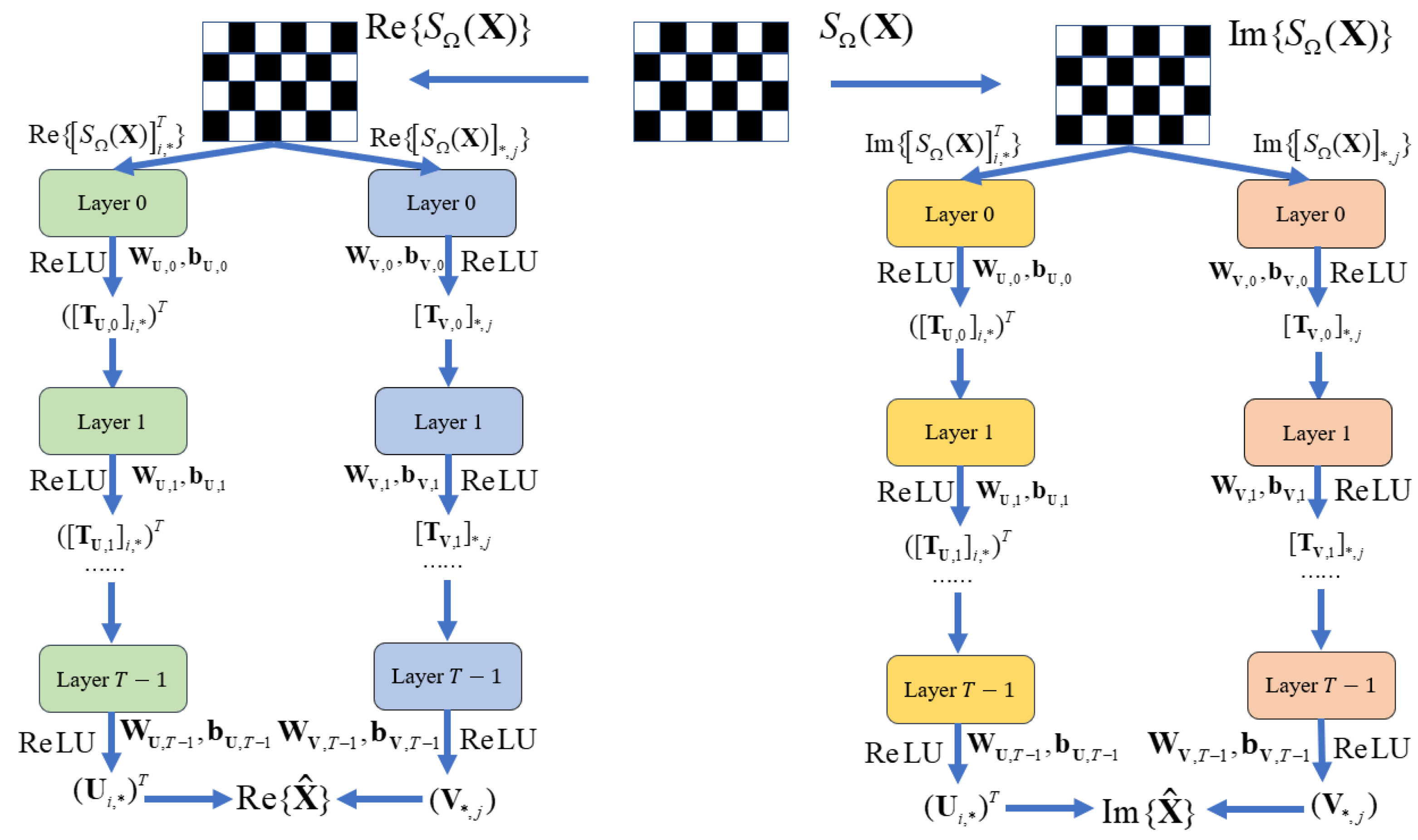
In this subsection, we present two methods, noted by the naive separation-of-real-and-imaginary-parts method and the real-valued representation-based method, respectively. The former method simply separates a complex-valued matrix into the real and imaginary parts, which are then independently proceeded by the corresponding neural networks. In the second approach, we propose a real-valued representation for the input complex-valued matrix and decompose the real-valued representation with the deep matrix factorization neural networks.

The basic idea of the first approach is illustrated in Figure 3, where the partially observed complex-valued matrix $S_{\mathrm{\Omega }}\left(\mathbf{X}\right)$ is separated into the real and imaginary parts. Then, we input the real and imaginary parts into two different neural networks with different weight and bias parameters, completing the real and imaginary parts of $\mathbf{X}$ separately. A drawback of this approach is that it discards the connection between the real and imaginary parts of $\mathbf{X}$. Since the real and imaginary parts of a low-rank complex-valued matrix are not necessarily of low rank themselves, this approach can result in bad completion performance. Therefore, to preserve the low-rank structure of the complex-valued matrix, we propose the second approach as discussed in sequel.

In the second approach, we consider an approximate real-valued reformulation of the complex-valued matrix completion problem [24]. For a complex-valued matrix $\mathbf{X}\in {\mathbb{C}}^{N_1\times N_2}$, we define a homomorphic mapping $\mathbf{R}\left(\mathbf{X}\right)\in {\mathbb{R}}^{2N_1\times 2N_2}$ as

$$\mathbf{R}\left(\mathbf{X}\right)=\left[\begin{array}{cc}\mathrm{Re}\left\{\mathbf{X}\right\}& \mathrm{Im}\left\{\mathbf{X}\right\}\\ -\mathrm{Im}\left\{\mathbf{X}\right\}& \mathrm{Re}\left\{\mathbf{X}\right\}\end{array}\right].$$

(9)

The ranks of these two matrices hold that $rank\left(\mathbf{R}\right(\mathbf{X}\left)\right)=2rank\left(\mathbf{X}\right),$ resulting from the following fact:

$$\begin{array}{c}\hfill {\mathbf{P}}_1^{-1}\mathbf{R}\left(\mathbf{X}\right){\mathbf{P}}_2=\left[\begin{array}{cc}\mathbf{X}& \\ & \overline{\mathbf{X}}\end{array}\right]\end{array},$$

(10)

where ${\mathbf{P}}_1\in {\mathbb{C}}^{2N_1\times 2N_1}$, ${\mathbf{P}}_2\in {\mathbb{C}}^{2N_2\times 2N_2}$ are expressed as

$$\begin{array}{c}\hfill {\mathbf{P}}_1=\left[\begin{array}{cc}{\mathbf{I}}_1& j{\mathbf{I}}_1\\ j{\mathbf{I}}_1& {\mathbf{I}}_1\end{array}\right],\end{array}$$

(11)

$$\begin{array}{c}\hfill {\mathbf{P}}_2=\left[\begin{array}{cc}{\mathbf{I}}_2& j{\mathbf{I}}_2\\ j{\mathbf{I}}_2& {\mathbf{I}}_2\end{array}\right],\end{array}$$

(12)

with ${\mathbf{I}}_1\in {\mathbb{C}}^{N_1\times N_1}$, ${\mathbf{I}}_2\in {\mathbb{C}}^{N_2\times N_2}$ being identity matrices.

Since the real-valued matrix $\mathbf{R}\left(\mathbf{X}\right)$ also has a low-rank structure like $\mathbf{X}$, current low-rank matrix completion methods designed for a real-valued matrix are also applicable to $\mathbf{R}\left(\mathbf{X}\right)$. Thus, $S_{\mathrm{\Omega }}\left(\mathbf{X}\right)$ can be recovered from the completion of matrix $\mathbf{R}\left(S_{\mathrm{\Omega }}\left(\mathbf{X}\right)\right)$.

The time complexity of the proposed DMF-Rr is

$$O\left({\displaystyle \sum _{l=1}^T}\left(N_1+N_2\right)M_{l-1}{M}_l\right).$$

(13)

where $N_1$ and $N_2$ denote the dimensions of the input matrix and $M_{l-1}$ and $M_l$ represent the input dimension and output dimension of the hidden layer in the neural network, respectively.

(2)

Enabling Complex-valued Operations with Real-valued Networks

In addition to the above approaches that reformulate complex-valued problems into real-valued ones, we propose here a method that modifies the structures of the neural network to enable complex-valued operations, which is noted by the complex-valued deep matrix factorization algorithm [24]. The core idea of the proposed method is inherited from [26], where complex-valued matrix computations are realized by real-valued networks with some modifications to activation functions. Below, we provide a detailed example of one layer in this adjusted architecture.

Recall from Figure 2 that a fully connected layer is given by

$$\mathbf{y}=\mathbf{W}\mathbf{x}+\mathbf{b}.$$

(14)

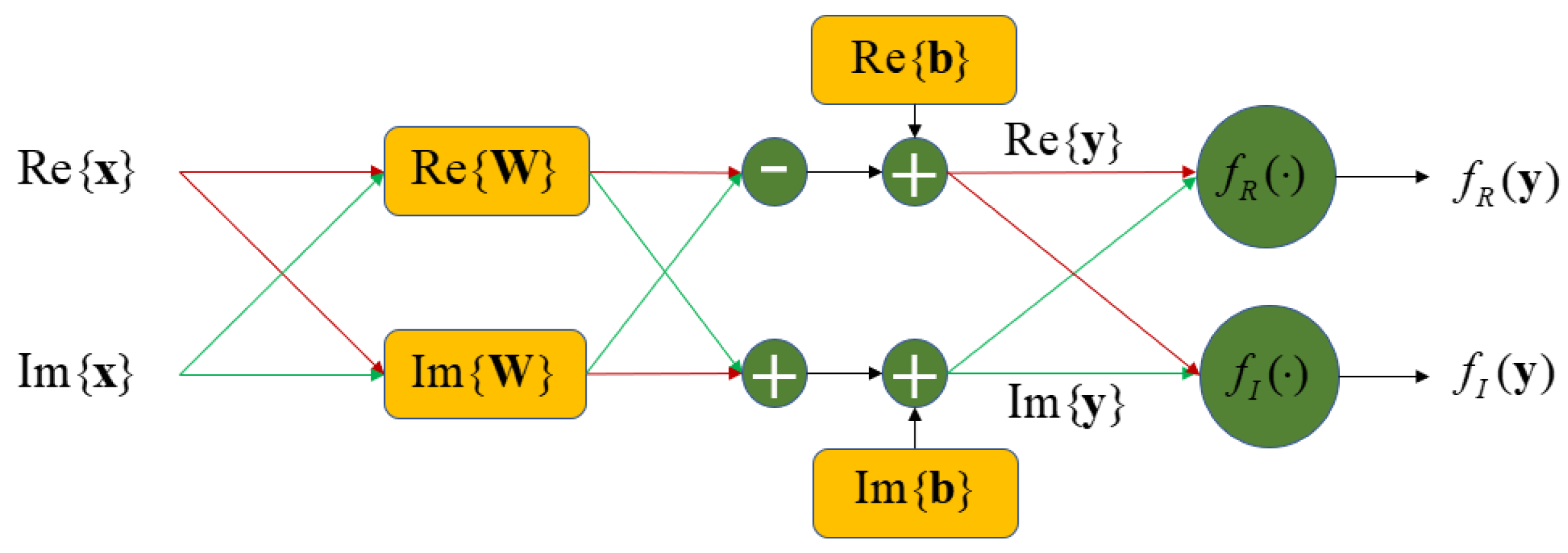
Here, for simplicity, we omit the superscripts and subscripts and use $\mathbf{y}\in {\mathbb{C}}^{M_l}$, $\mathbf{x}\in {\mathbb{C}}^{M_{l-1}}$, $\mathbf{W}\in {\mathbb{C}}^{M_l\times M_{l-1}}$ and $\mathbf{b}\in {\mathbb{C}}^{M_l}$ to represent the output feature vector, input feature vector, weight matrix, and bias vector, respectively. For complex-valued cases, (14) is rewritten as

$$\mathrm{Re}\left\{\mathbf{y}\right\}=\mathrm{Re}\left\{\mathbf{W}\right\}\mathrm{Re}\left\{\mathbf{x}\right\}-\mathrm{Im}\left\{\mathbf{W}\right\}\mathrm{Im}\left\{\mathbf{x}\right\}+\mathrm{Re}\left\{\mathbf{b}\right\},$$

(15)

$$\mathrm{Im}\left\{\mathbf{y}\right\}=\mathrm{Im}\left\{\mathbf{W}\right\}\mathrm{Re}\left\{\mathbf{x}\right\}+\mathrm{Re}\left\{\mathbf{W}\right\}\mathrm{Im}\left\{\mathbf{x}\right\}+\mathrm{Im}\left\{\mathbf{b}\right\}.$$

(16)

These equations inspire us to use the modified neural network structures, shown in Figure 4. Here, the real and imaginary parts of the complex-valued vector are input separately. They are then processed with the real and imaginary parts of the weight matrices $\mathbf{W}$, bias vectors $\mathbf{b}$, and activation functions $f_R(·)$, $f_I(·)$, resulting in the real and imaginary parts of the output vector, respectively.

In addition, the activation function should be changed accordingly. Here, we consider the softmax activation function, for a real-valued vector $\mathbf{y}$, which is

$$\begin{array}{c}\hfill f\left(y_i\right)={\displaystyle \frac{e^{y_i}}{{\sum }_{j=0}^{M_l-1}{e}^{y_j}}},\end{array}$$

(17)

with $y_i$ being the i-th entry of $\mathbf{y}$. The exponential term $e^{y_i}$ in the denominator should be extended to $e^{|y_i|}$ for a complex-valued entry. Additionally, inspired by the Swish activation function [29], we further replace the exponential term $e^{|y_j|}$ in the numerator with a linear term. Therefore, the activation function for the real part becomes

$$\begin{array}{c}\hfill f_R\left(y_i\right)={\displaystyle \frac{\mathrm{Re}\left\{y_i\right\}}{{\sum }_{j=0}^{M_l-1}{e}^{|y_j|}}},\end{array}$$

(18)

and the imaginary counterpart appears similarly. Consequently, the complex-valued output of the activation function is

$$\begin{array}{c}\hfill f_R\left(y_i\right)+j{f}_I\left(y_i\right)={\displaystyle \frac{y_i}{{\sum }_{j=0}^{M_l-1}{e}^{|y_j|}}}.\end{array}$$

(19)

For complex-valued numbers, one may also use other activation functions; an alternative approach is to change the exponent $e^{y_i}$ in the softmax activation function to the modulus of the complex-valued number $e^{|y_i|}$, as

$$\begin{array}{c}\hfill f\left(y_i\right)={\displaystyle \frac{e^{|y_j|}}{{\sum }_{j=0}^{M_l-1}{e}^{|y_j|}}}.\end{array}$$

(20)

However, this approach loses the phase information of the complex-valued number. As validated later in the subsequent experiment section, it is validated that this activation function is less effective than the proposed counterpart (19).

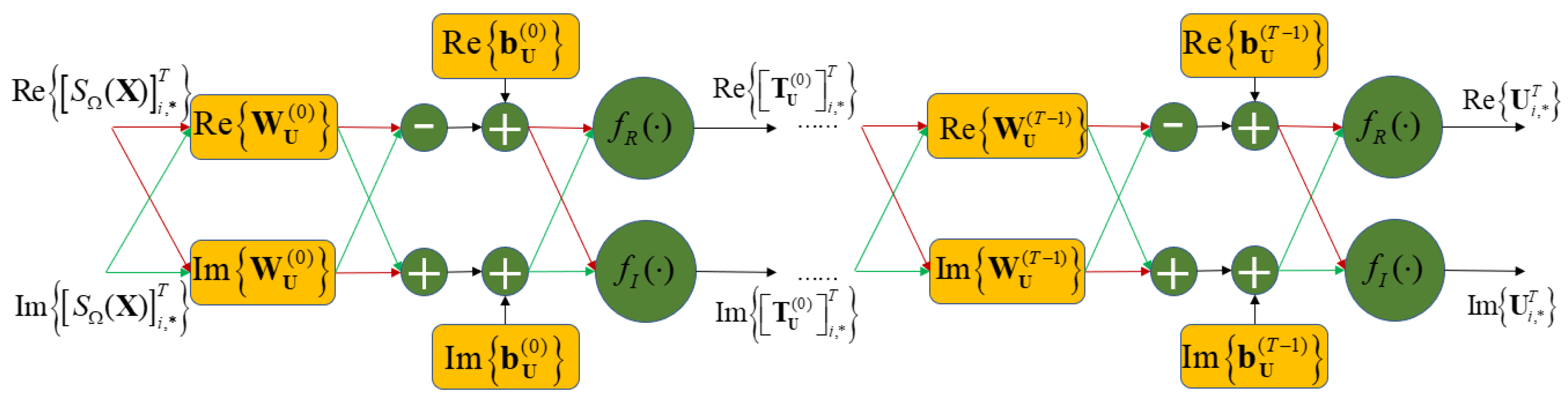
We summarize the architecture of complex-valued deep matrix factorization in Figure 5, where we take the network for generating $\mathbf{U}$ as an example. Now, the updated neural network is feasible for completing complex-valued matrices.

The time complexity of CDMF can also be formulated as (13). Compared with traditional matrix completion algorithms, the proposed CDMF and DMF-Rr achieve superior performance in terms of parameter estimation accuracy, signal matrix recovery quality, and beamforming results. However, due to the AI-enabled network structures and nonlinear mapping capabilities, the time complexity and computational cost of the proposed algorithms are relatively higher. Therefore, when deploying them on resource-constrained hardware platforms such as spaceborne platforms and edge devices, further optimization is still required via model lightweighting, network pruning, and inference acceleration techniques to meet the real-time and low-power consumption requirements in practical engineering applications.

3. Applications of Complex-Valued Matrix Completion on FDA Signal

Since complex-valued matrices have wide-ranging applications, the complex-valued matrix completion problem needs to be addressed in many fields. In this section, we mainly focus on signal processing for FDA radar [7,8,9,12,13], an example application of complex-valued matrix completion. In Section 3.1, we introduce the signal model for FDA radar. In Section 3.2, we introduce the low-rank structure of the FDA signal matrix. In Section 3.3, we discuss the procedure of FDA radar signal processing and explain how to apply complex-valued matrix completion for FDA radar signal processing.

3.1. FDA Signal Model

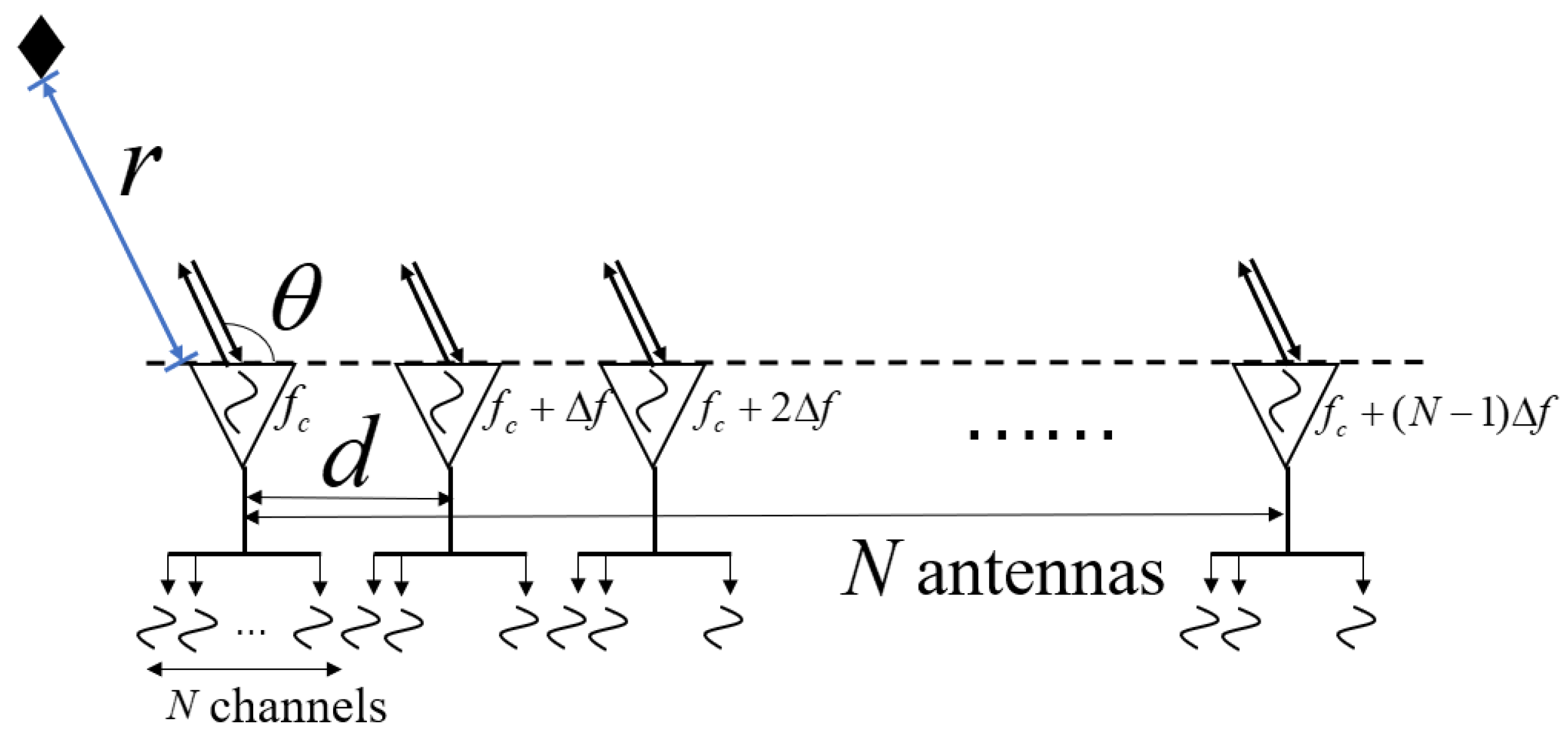
Consider an FDA which has N antennas with an interval d between two neighboring antennas, shown in Figure 6. The transmit carrier frequency of the first antenna is $f_c$, and the carrier frequencies of the other antennas increase successively by $\Delta f$. Here, we assume that $f_c\gg N\Delta f$. For the n-th antenna, $n\in \mathcal{N}=\{0,1,\dots ,N-1\}$, the transmitted signal is expressed as

$$s_n\left(t\right)=\exp \left\{j2\pi (f_c+n\Delta f)t\right\}.$$

(21)

We assume that the FDA is used to estimate a target with a scattering coefficient $\alpha$ at a range r and angle $\theta$, where the range r is sufficiently large, satisfying $r\gg Nd\sin \theta$. Each antenna receives radar returns originally transmitted by all N antennas. These signals are divided into N channels based on their carrier frequencies. The signal received by the m-th antenna in the n-th channel, where $m\in \mathcal{N}$, is given by

$$\begin{array}{c}\hfill r_{nm,F}\left(t\right)=\alpha \exp \left\{j2\pi (f_c+n\Delta f)\left(t-{\displaystyle \frac{2r}{c}}-{\displaystyle \frac{nd\sin \theta }{c}}-{\displaystyle \frac{md\sin \theta }{c}}\right)\right\}.\end{array}$$

(22)

We apply down-frequency conversion to the received signal, yielding

$$\begin{array}{cc}\hfill b_{nm,F}& =r_{nm,F}\left(t\right)\exp \{-j2\pi (f_c+n\Delta f)t\}\hfill \\ \hfill & \begin{array}{cc}\hfill =\alpha \exp & \left\{-j2\pi \left(n\left({\displaystyle \frac{2r\Delta f}{c}}+{\displaystyle \frac{f_{c}d\sin \theta }{c}}\right)+m{\displaystyle \frac{f_{c}d\sin \theta }{c}}+{\displaystyle \frac{n^2\Delta fd\sin \theta }{c}}\right.\right.\hfill \\ \hfill & \left.\left.+{\displaystyle \frac{mn\Delta fd\sin \theta }{c}}+{\displaystyle \frac{2r{f}_c}{c}}\right)\right\}.\hfill \end{array}\hfill \end{array}$$

(23)

Due to the assumptions $f_c\gg N\Delta f$ and $r\gg Nd\sin \theta$, one has that $2nr\Delta f\gg n^2\Delta fdsin\theta$, $n{f}_{c}dsin\theta \gg n^2\Delta fdsin\theta$, so the quadratic term involving $n^2$ and the coupling term involving $mn$ can be neglected. We define $\gamma =\alpha \exp \{(-j4\pi r{f}_c)/c\}$ as the equivalent scattering coefficient of the target. Thus, the signal after down-conversion processing is expressed as

$$\begin{array}{c}\hfill b_{nm,F}\approx \gamma \exp \left\{-j2\pi \left(n\left({\displaystyle \frac{2r\Delta f}{c}}+{\displaystyle \frac{f_{c}d\sin \theta }{c}}\right)+m{\displaystyle \frac{f_{c}d\sin \theta }{c}}\right)\right\}.\end{array}$$

(24)

When there are K targets, (24) can be written as

$$\begin{array}{cc}\hfill b_{nm,F}\approx {\displaystyle \sum _{k=0}^{K-1}}{\gamma }_k\exp & \left\{-j2\pi \left({\displaystyle \frac{n\left(2r_k\Delta f+f_{c}d\sin {\theta }_k\right)}{c}}+{\displaystyle \frac{m{f}_{c}d\sin {\theta }_k}{c}}\right)\right\},\hfill \end{array}$$

(25)

where $r_k$ is the range of the k-th target, ${\theta }_k$ is its angle, and ${\gamma }_k$ is its equivalent scattering coefficient.

For the spaceborne FDA scenario for space debris detection presented in this paper, the above theoretical model has a certain influence. However, according to the simulation results by Zhao et al. [30], although their experimental setup was based on a millimeter-wave phased array radar and certain approximations were made for the radar cross section of space debris, the theoretical model can still be considered applicable to space debris.

Now we rewrite (25) into matrix form by defining $\mathbf{Y}\in {\mathbb{C}}^{N\times N}$ with its $(n,m)$-th entry given by

$$\begin{array}{c}\hfill {\left[\mathbf{Y}\right]}_{n,m}=b_{nm,F}.\end{array}$$

(26)

In random FDA radars, each antenna only receives signals from random Q channels. Therefore, the random FDA signal matrix ${\mathbf{Y}}_R\in {\mathbb{C}}^{N\times N}$ can be seen as a random sampling of $\mathbf{Y}$. Let $\mathrm{\Omega }$ be a sampling set of a matrix, expressed as

$$\mathrm{\Omega }=\left\{(q,m)\right|q\in {\mathcal{Q}}_m,m\in \mathcal{N}\},$$

(27)

where $\mathcal{N}$ is the set of antenna indexes and ${\mathcal{Q}}_m=\{q_{m,0},q_{m,1},...,q_{m,Q-1}\}\subset \mathcal{N}$ is the index set of the Q sampled channels for the m-th antenna. From (1) and (2), the sample of $\mathbf{Y}$ on $\mathrm{\Omega }$ can be expressed as

$$\begin{array}{c}\hfill {\left[S_{\mathrm{\Omega }}\left(\mathbf{Y}\right)\right]}_{i,j}=\left\{\begin{array}{c}{\left[\mathbf{Y}\right]}_{i,j},\mathrm{if}(i,j)\in \mathrm{\Omega },\hfill \\ 0,\mathrm{else}.\hfill \end{array}\right.\end{array}$$

(28)

Then, we express the random FDA’s signal matrix ${\mathbf{Y}}_R$ as the sample of $\mathbf{Y}$ on $\mathrm{\Omega }$, given by ${\mathbf{Y}}_R=S_{\mathrm{\Omega }}\left(\mathbf{Y}\right).$

3.2. Low-Rank Structure of FDA Signal Matrix

To reveal the low-rank structure of $\mathbf{Y}$, we decompose the matrix $\mathbf{Y}$ as

$$\begin{array}{c}\hfill \mathbf{Y}={\mathbf{Y}}_1{\mathbf{Y}}_2^T,\end{array}$$

(29)

where ${\mathbf{Y}}_1\in {\mathbb{C}}^{N\times K}$, ${\mathbf{Y}}_2\in {\mathbb{C}}^{N\times K}$ can be expressed as

$$\begin{array}{c}\hfill {\left[{\mathbf{Y}}_1\right]}_{n,k}=\sqrt{{\gamma }_k}\exp \left\{-j2\pi \left({\displaystyle \frac{n\left(2r_k\Delta f+f_{c}d\sin {\theta }_k\right)}{c}}\right)\right\},\end{array}$$

(30)

$$\begin{array}{c}\hfill {\left[{\mathbf{Y}}_2\right]}_{m,k}=\sqrt{{\gamma }_k}\exp \left\{-j2\pi \left({\displaystyle \frac{m{f}_{c}d\sin {\theta }_k}{c}}\right)\right\},\end{array}$$

(31)

so we know that the rank of the matrix satisfies $rank\left(\mathbf{Y}\right)\le K$. Therefore, recovering the missing data is possible. By exploiting the low-rank structure, one recovers the missing data in ${\mathbf{Y}}_R$ and obtains an estimation of the full observation matrix $\mathbf{Y}$. However, there exist several scenarios where the low-rank property of the matrix breaks down. In the presence of abundant multipath, dense scattering, or strong clutter, the rank of the signal matrix is no longer dominated by a small number of targets, and its effective rank increases significantly [31]. However, in space debris detection missions, the scenario is generally sparse, and the influence caused by multipath effects is limited. Therefore, the problem of multipath suppression in space debris detection will be addressed in future work. When Doppler spread or target motion exists, the ideal spatial-frequency coupling structure of the FDA is destroyed, and the rank is no longer determined by the number of targets [32]. When the Signal-to-Noise Ratio (SNR) of the targets is too low, noise becomes dominant in the signal matrix, so the low-rank assumption also ceases to hold.

3.3. FDA Signal Processing

Our goal is to estimate the unknown parameters of targets such as the ranges, angles and scattering coefficients from the fully known observations $\mathbf{Y}$ or partially known ${\mathbf{Y}}_R$. One typically uses the conventional beamforming algorithm, introduced below.

The conventional beamforming defines a matrix $\mathbf{C}\in {\mathbb{C}}^{N\times N}$ with the $(n,m)$-th entry as

$$\begin{array}{c}\hfill {\left[\mathbf{C}\right]}_{n,m}=\exp \left\{j2\pi \left(n\left({\displaystyle \frac{2\widehat{r}\Delta f}{c}}+{\displaystyle \frac{f_{c}d\sin \widehat{\theta }}{c}}\right)+m{\displaystyle \frac{f_{c}d\sin \widehat{\theta }}{c}}\right)\right\},\end{array}$$

(32)

where $\widehat{r}$ and $\widehat{\theta }$ are the search variables for range and angle, respectively. Then, calculating the inner product between $\mathbf{C}$ and the observation matrix yields

$$\begin{array}{c}\hfill y(\widehat{r},\widehat{\theta })={\displaystyle \sum _{n=0}^{N-1}}{\displaystyle \sum _{m=0}^{N-1}}{\left[\mathbf{C}\right]}_{n,m}{\left[\mathbf{Y}\right]}_{n,m}.\end{array}$$

(33)

Similarly for random FDA, the conventional beamforming results are

$$\begin{array}{c}\hfill y_R(\widehat{r},\widehat{\theta })={\displaystyle \sum _{n=0}^{N-1}}{\displaystyle \sum _{m=0}^{N-1}}{\left[\mathbf{C}\right]}_{n,m}{\left[{\mathbf{Y}}_R\right]}_{n,m}.\end{array}$$

(34)

The target ranges and angles are determined by the peak values of the conventional beamforming results.

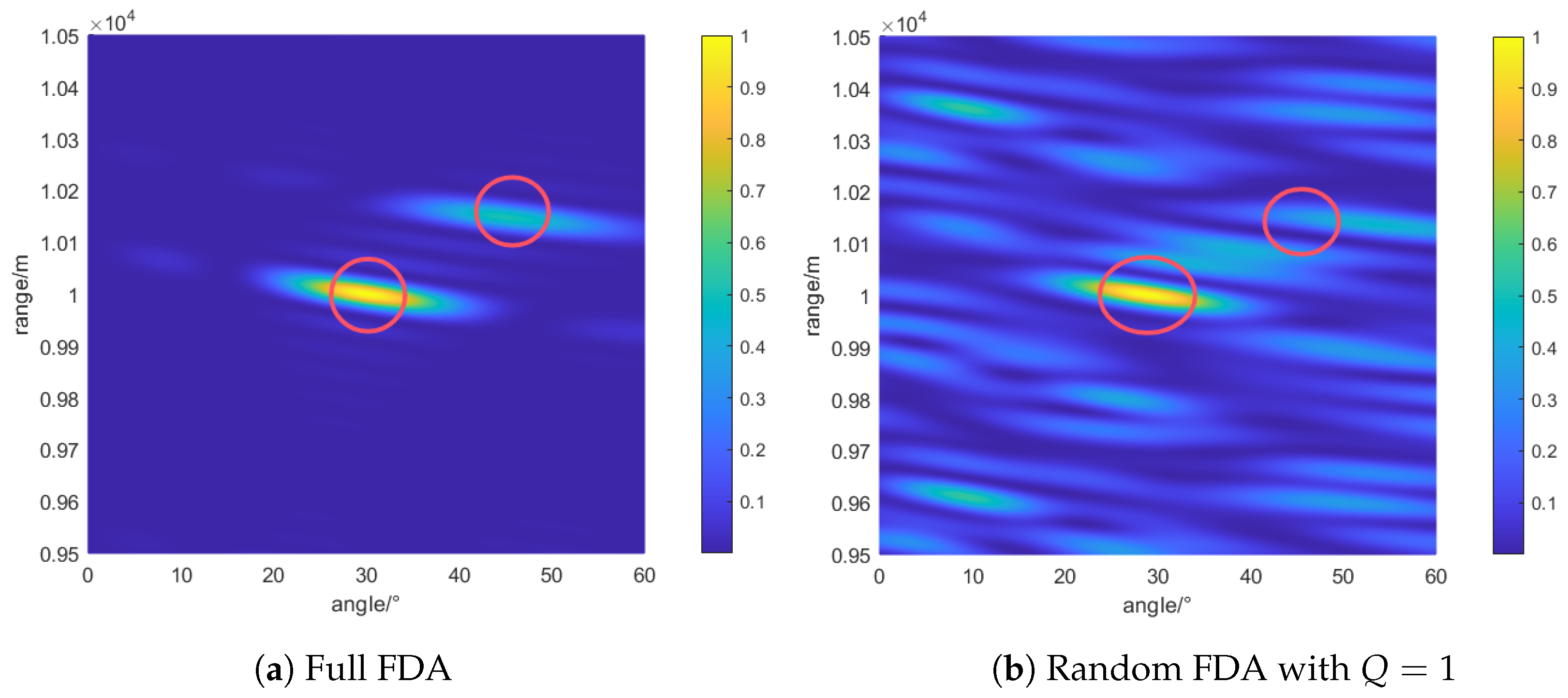
To illustrate the performance of conventional beamforming, we simulate a simple case with $N=16$ and two targets located at the ranges and angles of $(10 \mathrm{km}, 30°)$ and $(10.15 \mathrm{km}, 45°)$, respectively.

In the full FDA scenario, the conventional beamforming results of the received signals $\left|y\right(\widehat{r},\widehat{\theta }\left)\right|$ are shown in Figure 7a, where the two peaks in the conventional beamforming results correspond to the locations of the targets.

In the random FDA scenario, with $Q=1$, the channel set for the m-th receive antenna is ${\mathcal{Q}}_m=\left\{q_{m,0}\right\}$, where $q_{m,0}$ represents the randomly selected channel index for the m-th receive antenna. The conventional beamforming results of the received signals are displayed in Figure 7b. Due to missing elements in ${\mathbf{Y}}_R$, the conventional beamforming results exhibit higher sidelobes compared to those from full observations shown in Figure 7a. These high sidelobes may obscure weak targets, highlighting the need for more advanced signal processing techniques: conducting matrix completion prior to beamforming. The specific signal processing procedure for the random FDA is shown in Algorithm 2.

Algorithm 2: Signal Processing Procedure for Random FDA
	Input: ${\mathbf{Y}}_R$: random FDA signal matrix; $\mathrm{\Omega }$: the sampling set of ${\mathbf{Y}}_R$.
1	Choose a matrix completion algorithm, such as AI-enabled CDMF and DMF-Rr;
2	Perform the selected matrix completion algorithm on ${\mathbf{Y}}_R$, yielding $\widehat{\mathbf{Y}}$;
3	Perform conventional beamforming on $\widehat{\mathbf{Y}}$, resulting in $y_R(\widehat{r},\widehat{\theta })$;
	Output: $y_R(\widehat{r},\widehat{\theta })$.

For the random FDA radar, some entries are missing in its signal matrix during signal processing. These missing entries lead to high sidelobes when performing beamforming on the random FDA radar echo. To suppress such sidelobes, the AI-enabled CDMF and DMF-Rr proposed in Section 2 can be employed to first complete the incomplete signal matrix of the random FDA radar echo. Therefore, AI-Enabled FDA in this manuscript refers to the fact that the signal processing method for random FDA is AI-enabled. Then, beamforming is performed on the completed signal matrix, which achieves the goal of sidelobe suppression in the signal processing results of random FDA radar.

4. Numerical Experiments

In this section, to verify the effectiveness of the proposed methods, CDMF and DMF-Rr, in solving the complex matrix completion problem, we compare these two methods with three traditional methods: SVT [33], gradient-descent-based AltMinComplete (GD) and LMaFit. It is important to note that, since the objective function (5) in complex-valued matrix completion is non-analytic, the complex-valued gradient operator proposed by Brandwood [34] must be used when applying the gradient descent-based AltMinComplete algorithm. Furthermore, we also design ablation experiments to demonstrate the effectiveness of the model structure and activation function proposed for the complex-valued deep matrix factorization method. In the ablation experiments, we use deep matrix factorization on the real and imaginary parts (DMF-RI), which keeps the model structure unchanged, and complex-valued deep matrix factorization with softmax (DMF-NF), which keeps the activation function unchanged, as comparison. In Section 4.1, we compare the performance of these seven methods in completing random matrices by calculating the NMSE after applying these methods to random matrix completion. In Section 4.2, we compare their performance in completing FDA signal matrices by calculating both the normalized mean squared error (NMSE) after matrix completion and the root mean squared error (RMSE) after applying CBF to the completed FDA signal matrices. In Section 4.3, we simulate a scenario where a spaceborne FDA radar detects space debris.

4.1. Random Matrices

In this subsection, we first evaluate the performance of the traditional and the proposed matrix completion methods on randomly generated matrices. The size of the matrix is $20\times 20$, and when the rank r of the given matrix is set to 4, the missing rates $\delta$ are set to 30%, 50%, and 70%, respectively. When the missing rate $\delta$ of the given matrix is set to 50%, the ranks r are set to 4, 6, and 8, respectively. We use NMSE to evaluate the matrix completion performance, expressed as

$$\mathrm{NMSE}=\parallel \widehat{\mathbf{X}}{-\mathbf{X}\parallel }_F^2/{\parallel \mathbf{X}\parallel }_F^2.$$

(35)

The NMSE results of the proposed and traditional methods are shown in

Table 1. NMSEs of random matrix completion under different missing rates.

Missing Rates	SVT	GD	LMaFit	DMF-RI	DMF-NF	CDMF	DMF-Rr
$\delta =30\%$	0.0798	0.0604	0.0874	0.0819	0.7647	0.0307	0.0462
$\delta =50\%$	0.2004	0.3936	0.6107	0.2096	0.7441	0.0464	0.1511
$\delta =70\%$	0.4225	2.6226	0.8473	0.3003	0.7935	0.2616	0.2358

and

Table 2. NMSEs of random matrix completion under different ranks.

Ranks	SVT	GD	LMaFit	DMF-RI	DMF-NF	CDMF	DMF-Rr
$r=4$	0.2004	0.3936	$0.6107$	0.2096	0.7441	0.0464	0.1511
$r=6$	0.4871	1.9589	0.7984	0.2498	0.7935	0.2076	0.1751
$r=8$	0.5209	5.0575	0.9231	0.3003	0.9234	0.2347	0.1805

.

The NMSEs of the methods proposed in this paper and other traditional algorithms with varying missing rates and the ranks of the matrix are illustrated in Table 1 and Table 2. As can be seen from Table 1 and Table 2, with the increase in data missing rate and the rank of the matrix, the matrix completion performance of both the methods proposed and traditional algorithms degrades, but the performance of the methods proposed remains superior to that of traditional algorithms. This indicates that the methods proposed outperform traditional algorithms in complex-valued matrix completion across scenarios with different missing rates and matrix ranks.

This indicates that the two neural network-based complex-valued matrix completion methods proposed in this paper perform better than traditional methods in the cases of high missing rates. Additionally, when the missing rate is the same, the complex-valued deep matrix factorization’s method performs better than the real-valued representation-based method.

Through ablation experiments on the complex-valued deep matrix factorization method proposed in this paper, we can see that when we do not modify the neural network structures and directly complete the real and imaginary parts of the complex-valued matrix separately. The completion performance is inferior to that of the proposed complex-valued deep matrix factorization method. Furthermore, when we only modify the neural network structures without altering the activation functions, the experimental results show that the matrix completion performance is the worst in this case.

4.2. FDA Signal Matrices

In this subsection, we apply the two neural network-based complex-valued matrix completion methods proposed in this paper to the FDA signals mentioned in Section 3. We set the number of FDA antennas $N=16$, the initial carrier frequency $f_c=10\mathrm{GHz}$, the frequency increment step $\Delta f=200\mathrm{kHz}$ and the inter-element distance $d={\displaystyle \frac{c}{4f_c}}$. In Section 4.2.1, we compare the completion performance (i.e., NMSE) of the two methods proposed in this paper with traditional methods, and then we conduct ablation experiments on the two proposed methods to verify their effectiveness when applied to FDA signals. In Section 4.2.2, we compare the parameter estimation performance of the two proposed methods with traditional methods, where RMSE is expressed as

$$\mathrm{RMSE}=\sqrt{{\displaystyle \frac{1}{N_{monte}}}{\displaystyle \sum _{i=0}^{N_{monte}-1}}{\displaystyle \sum _{k=0}^{K-1}}{\widehat{r}}_k^2+r_k^2-2{\widehat{r}}_k{r}_{k}cos({\widehat{\theta }}_k-{\theta }_k)}.$$

(36)

Among them, $N_{monte}$ denotes the number of Monte Carlo simulations, ${\widehat{r}}_k$ and ${\widehat{\theta }}_k$ represent the estimated range and angle of the k-th target, respectively, while $r_k$ and ${\theta }_k$ denote the true range and angle of the k-th target. Then, we conduct ablation experiments to verify the effectiveness of these methods for parameter estimation on FDA signals.

4.2.1. Effectiveness of FDA Signal Matrix Completion

In this subsection, we applied matrix completion algorithms to restore the signal matrix for random FDA signals under different receiving channels Q with a fixed number of targets $K=2$, with (range, angle, scattering intensity) being $(10 \mathrm{km}, 30°, -17 \mathrm{dB})$ and $(10.15 \mathrm{km}, 45°, -20 \mathrm{dB})$, respectively. The restoration effectiveness is shown in

Table 3. NMSEs of the recovered FDA signal matrices with a fixed number of targets under different numbers of receiving channels Q [24].

Q	SVT	GD	LMaFit	DMF-RI	DMF-NF	CDMF	DMF-Rr
1	0.9541	7.7403	0.9641	0.5829	0.9337	0.5560	0.4745
2	0.8611	4.6700	0.9006	0.5760	0.7986	0.5323	0.3365
3	0.7635	3.2918	0.6094	0.3656	0.7491	0.2408	0.2869
4	0.6308	2.9558	0.2341	0.2396	0.7319	0.0229	0.1600
5	0.5538	2.3283	0.0437	0.2047	0.9265	0.0246	0.0517
6	0.5124	2.9068	$4.154\times {10}^{-9}$	0.2037	0.7620	0.0112	0.0207

.

As seen in Table 3, when $Q\le 3$, the NMSEs of the two complex-valued matrix completion methods proposed in this paper are lower than those of the traditional methods. However, when $Q=6$, the NMSE of the LMaFit is significantly lower than that of the proposed methods. This is consistent with the conclusion in Section 4.1 that the methods proposed in this paper perform better when dealing with matrices of a high missing rates.

To compare the effectiveness of the following methods, i.e., complex-valued deep matrix factorization proposed in this paper, the complex-valued deep matrix factorization method without modifying the activation function, and the method that performs deep matrix factorization on the real and imaginary parts of the complex-valued matrix, we applied them to the random FDA signal recovering problem. Their NMSEs are also shown in Table 3.

From the results of the ablation experiments in Table 3, we see that the complex-valued deep matrix factorization method proposed in this paper achieves the best performance in FDA signal matrix completion, followed by performing deep matrix factorization on the real and imaginary parts separately, while the complex-valued deep matrix factorization method without modifying the activation function performs the worst. Therefore, it can be concluded that the two proposed methods for the complex-valued deep matrix factorization method, which adjust neural network structures and activation functions, are more effective.

We then applied matrix completion algorithms to recover the signal matrix of random FDA signals with a fixed number of receiving channels $Q=4$ under different numbers of targets K. The three targets’ parameters (range, angle, scattering intensity) are set as $(10 \mathrm{km}, 30°, 20 \mathrm{dB})$, $(10.15 \mathrm{km}, 45°, 17 \mathrm{dB})$ and $(9.85 \mathrm{km}, 15°, 17 \mathrm{dB})$. The restoration effectiveness is shown in

Table 4. NMSEs of recovered FDA signal matrices with a fixed number of receiving channels $Q=4$ under different numbers of targets K [24].

K	SVT	GD	LMaFit	DMF-RI	DMF-NF	CDMF	DMF-Rr
1	0.5956	2.0000	0.0625	0.0909	0.7036	0.0280	0.0093
2	0.6308	2.9558	0.2341	0.2396	0.7319	0.0229	0.1600
3	0.6641	7.2263	2.6939	0.4287	0.8752	0.2025	0.2831

. As shown in Table 4, when the number of receiving channels is fixed as $Q=4$, the complex-valued deep matrix factorization method proposed in this paper outperforms the traditional methods.

To demonstrate the effectiveness of the complex-valued deep matrix factorization proposed in this paper, we conducted ablation experiments on this method under the given conditions. The experimental results are also shown in Table 4. When the number of receiving channels is fixed at $Q=4$, under different numbers of targets, the complex-valued deep matrix factorization method proposed in this paper achieves the best performance in FDA signal matrix completion, followed by performing deep matrix factorization on the real and imaginary parts, with the complex-valued deep matrix factorization method without modifying the activation function performing the worst. Therefore, it can be concluded that the two proposed methods for the complex-valued deep matrix factorization method, targeting neural network structures and activation functions, are effective.

4.2.2. FDA Radar Target Parameter Estimation

In this subsection, based on the completed signal matrix, we use the conventional beamforming algorithm to estimate parameters, and we evaluate the impact of each matrix completion method on the parameter estimation results.

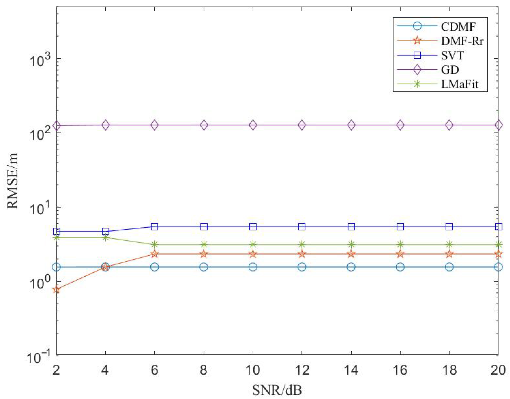
With the number of targets K and the number of receive channels Q fixed, beamforming was performed on the random FDA radar signal matrix completed by the CDMF and various traditional algorithms. A total of 500 independent Monte Carlo experiments were repeated to calculate the RMSE, and the results are shown in Figure 8. It can be observed from Figure 8 that when the number of receive channels Q and the number of targets K are fixed, the parameter estimation RMSE values of the proposed CDMF and DMF-Rr algorithms are lower than those of other traditional methods as the SNR increases, which demonstrates the superiority of the CDMF and DMF-Rr algorithms in random FDA radar signal processing tasks.

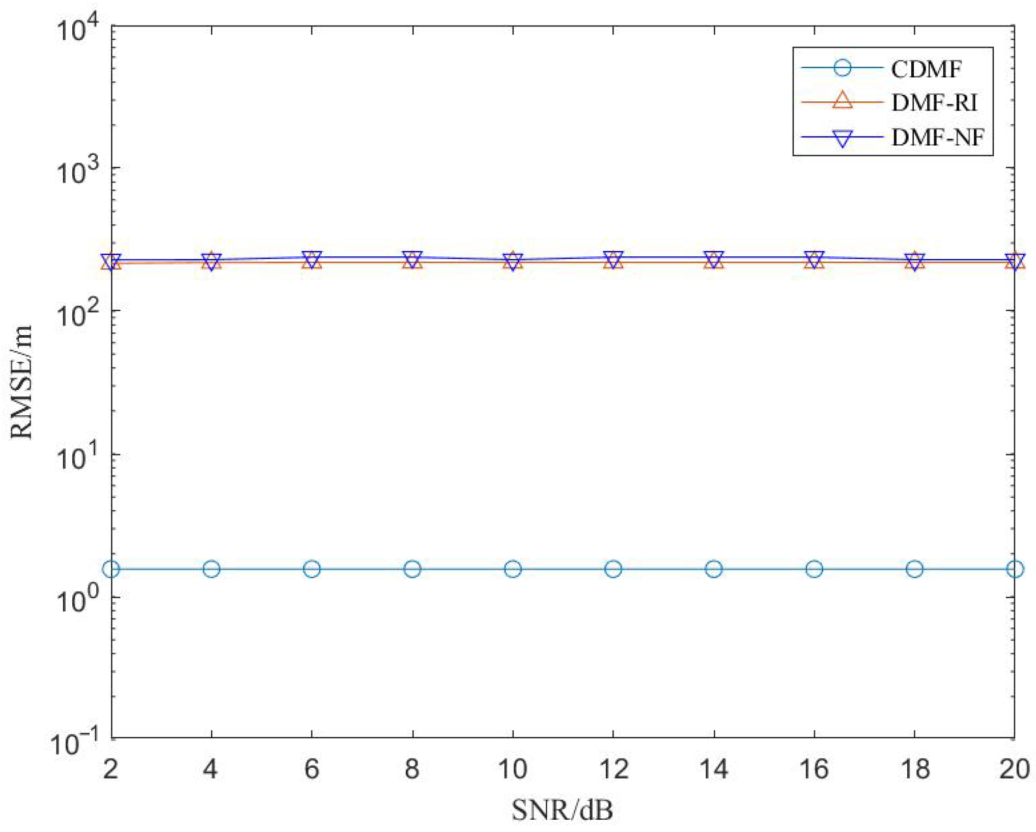
It is observed from the ablation experiments that with the number of targets and the number of receive channels fixed, ablation experiments were carried out on the proposed CDMF. We repeated 500 Monte Carlo trials and calculated the RMSE, with the results shown in Figure 9. It can be observed from the ablation experiments that as the SNR varies; the RMSE of the proposed CDMF is significantly lower than that of the other methods. This result verifies the effectiveness of the improved network structure and activation function proposed in this paper for the parameter estimation task in random FDA radar.

4.3. FDA Radar Detects Space Debris

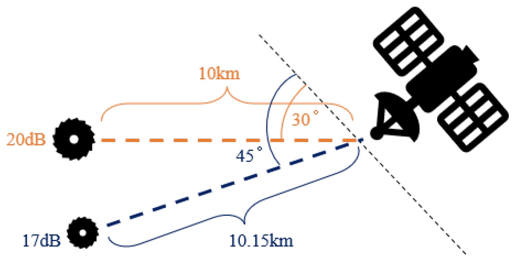
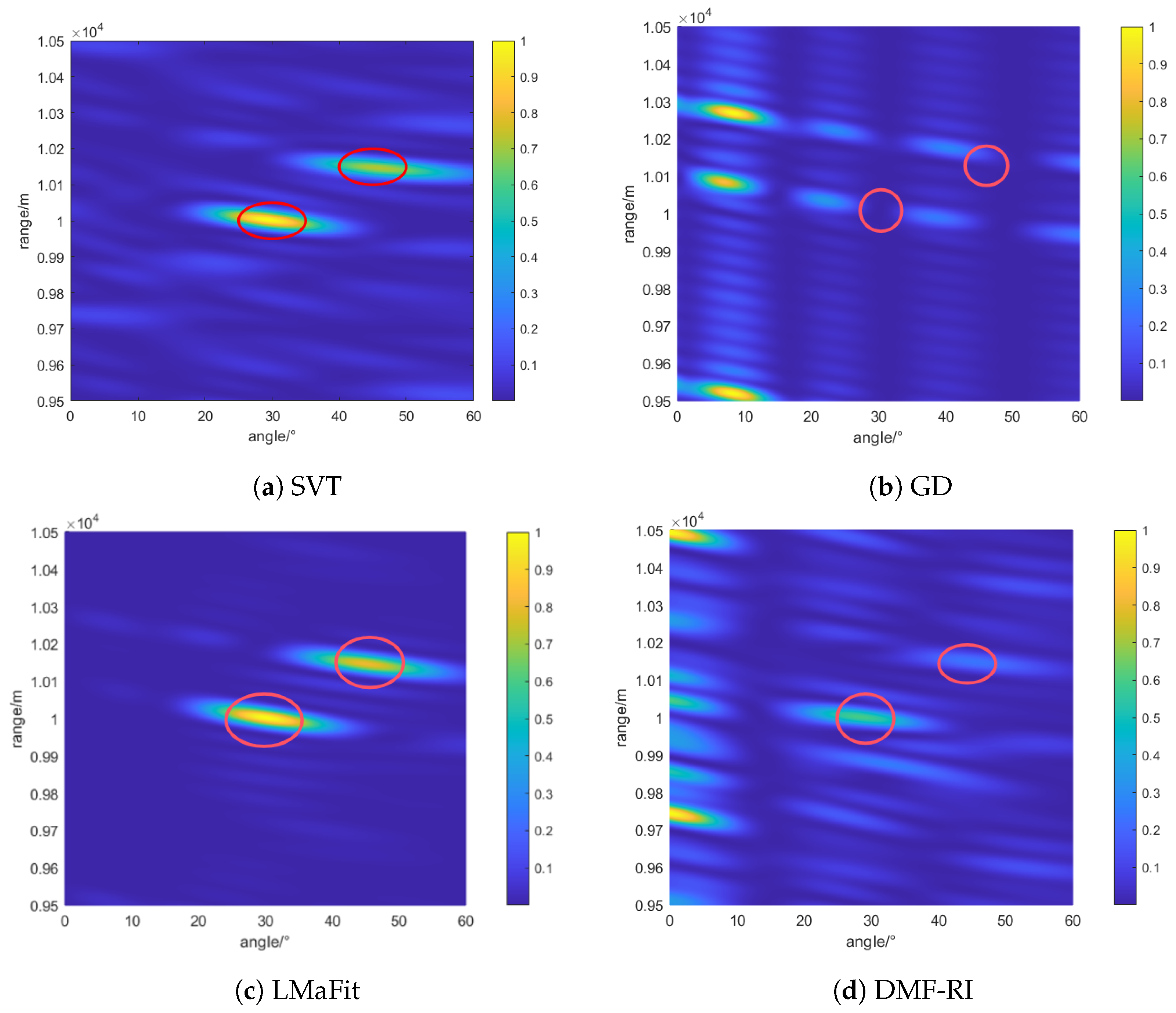
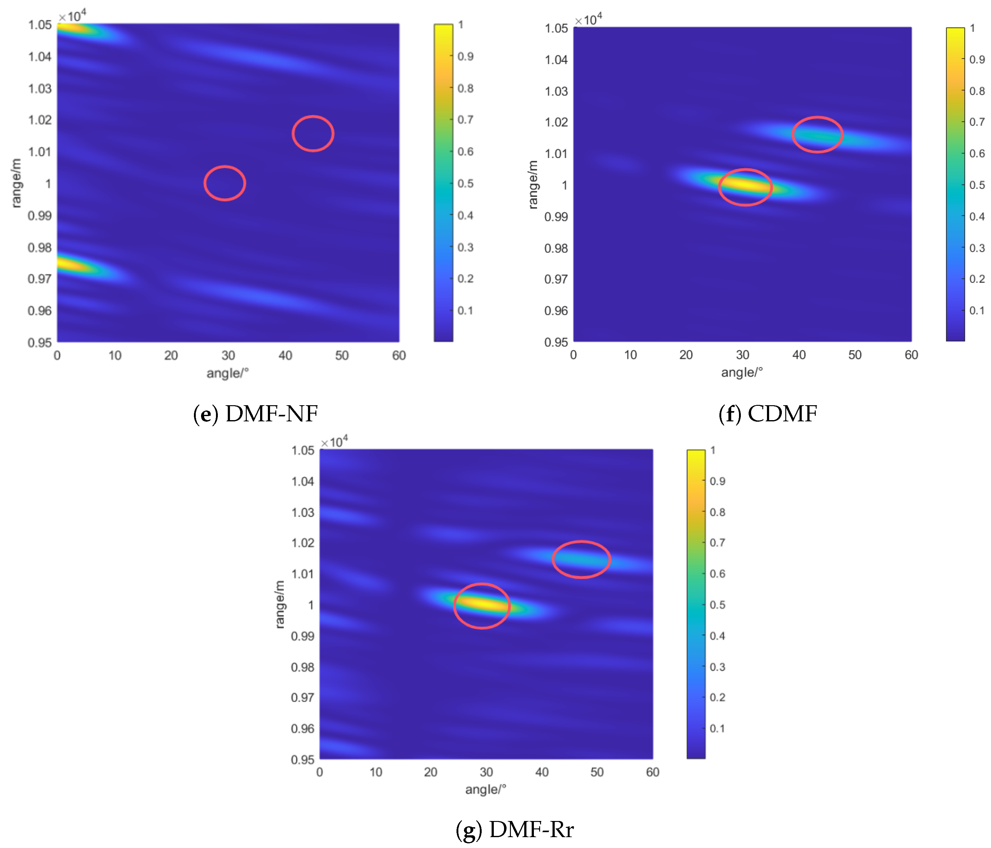
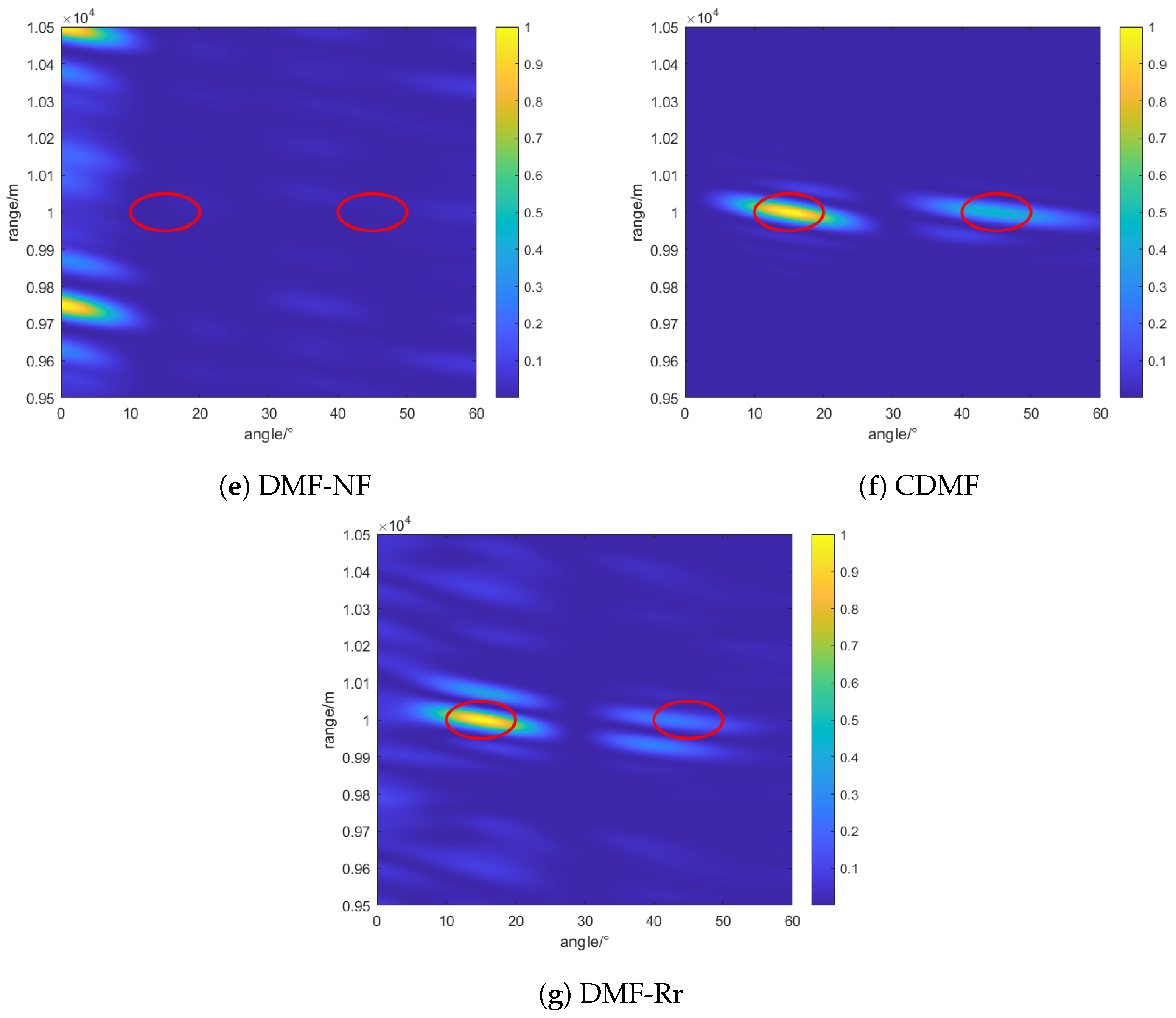
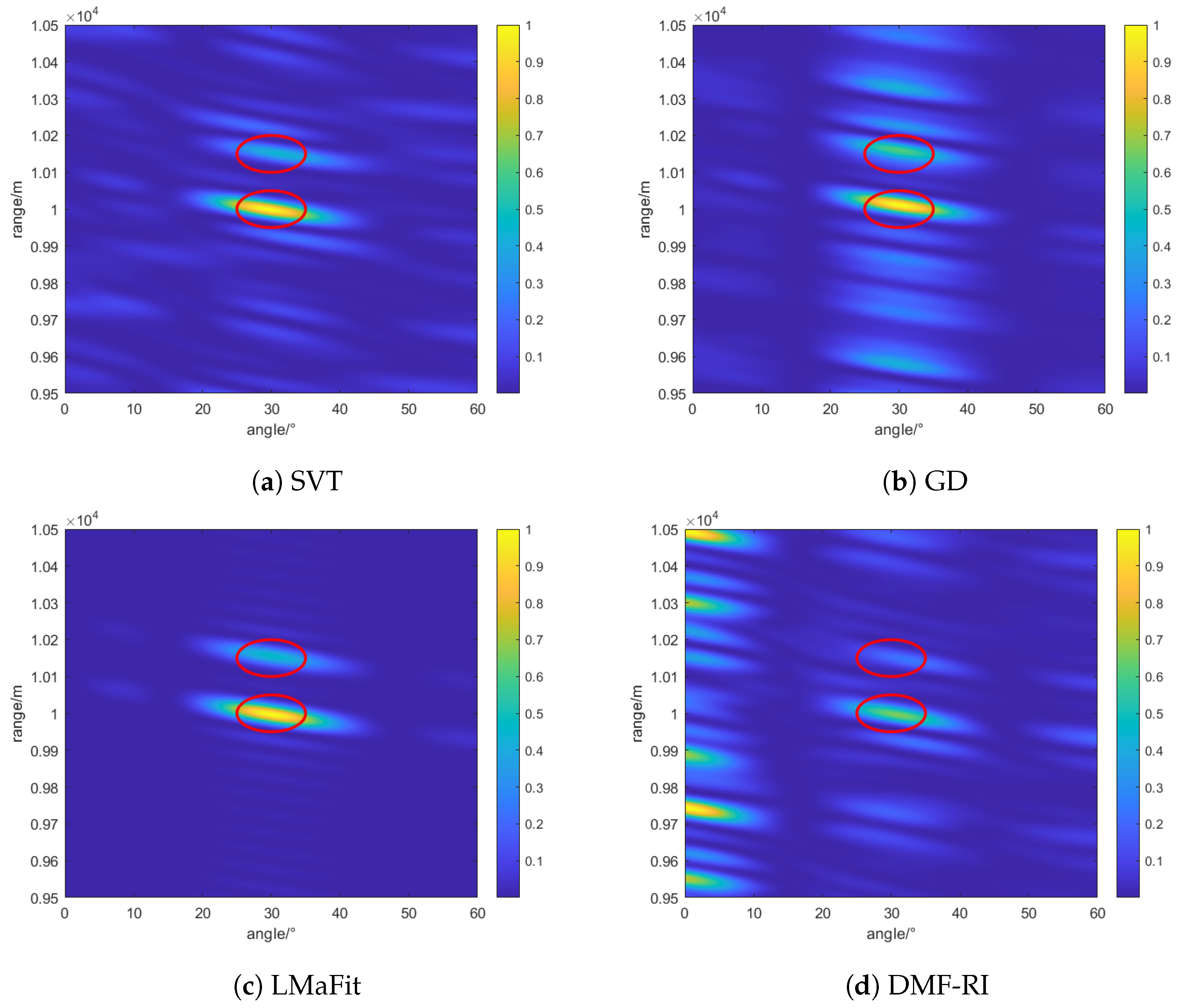
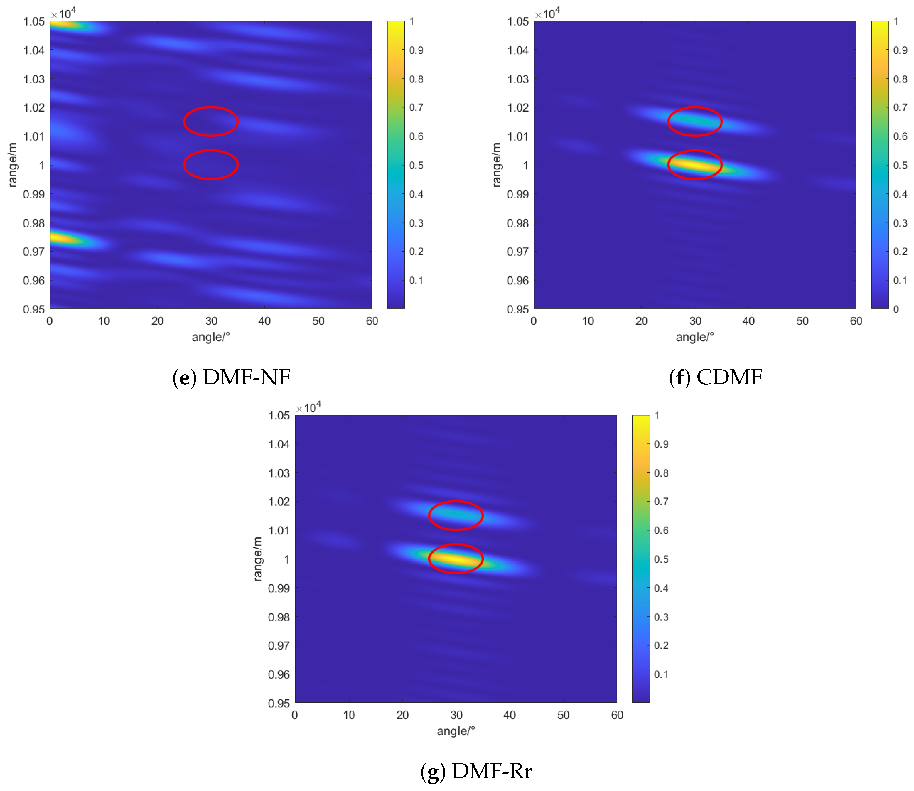
When a spaceborne random FDA radar is used for space debris detection, it is assumed that there are two pieces of space debris in the simulation scenario, with the distance, angle and signal-to-noise ratio relative to the spaceborne random FDA radar being $(10\mathrm{km}, 30°, 20\mathrm{dB})$ and $(10.15\mathrm{km}, 45°, 17\mathrm{dB})$, respectively, as shown in Figure 10. The parameter settings of the spaceborne FDA radar are consistent with those in Section 4.2. Based on the completed signal matrix, this section adopts the beamforming algorithm to carry out parameter estimation and evaluates the impact of various matrix completion methods on the space debris detection performance. With the number of targets K and the number of receive channels Q fixed, the beamforming results of the random FDA radar signal matrix completed by the CDMF and various traditional algorithms are shown in Figure 11. With the results shown in Figure 11c,f,g, both the proposed algorithms and the LMaFit algorithm can effectively estimate the target parameters at the positions marked by the red circles, which are close to the beamforming results of the conventional FDA. With the results shown in Figure 11a, the range-angle beam map obtained by beamforming the signal matrix recovered by the SVT has relatively high sidelobes, which is similar to the result of the incomplete signal matrix. In contrast, with the results shown in Figure 11b, the range-angle beam map based on the signal matrix completed by the GD algorithm exhibits the highest sidelobes. When the number of targets K and the number of receive channels Q are fixed, the ablation experiments of CDMF are illustrated in Figure 11d,e. It can be observed that the beam pattern obtained by CDMF after random FDA signal matrix completion can effectively estimate the target parameters at the positions marked by the red circles. However, the method of separately completing the real and imaginary parts and the method using the Softmax activation function fail to provide accurate estimation of target parameters after signal matrix completion. Therefore, it can be concluded that with a fixed number of receive channels Q and targets K, the adjusted neural network structure and activation function proposed in this paper achieve superior performance for parameter estimation in random FDA radar.

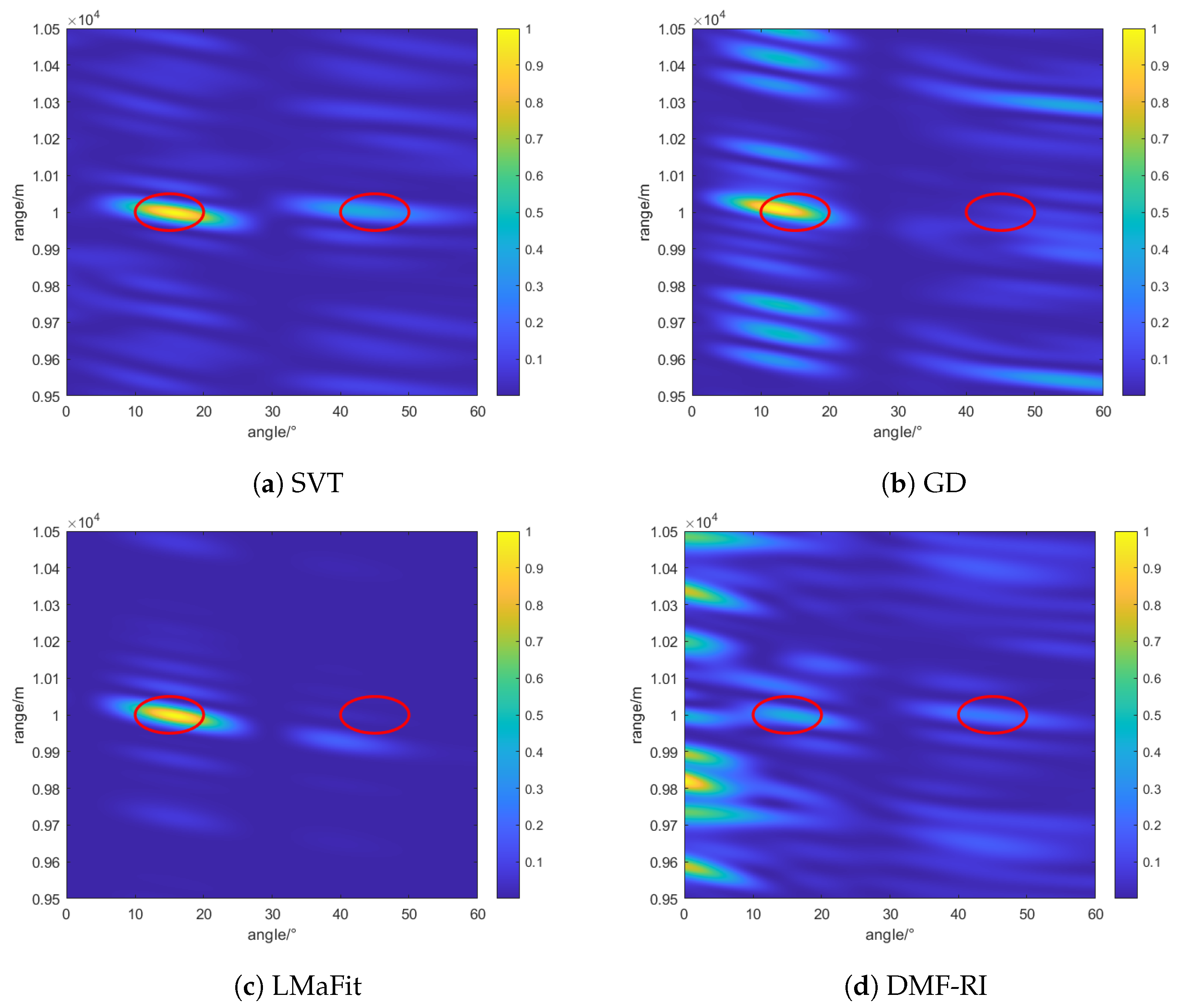
As shown in Figure 12 and Figure 13, although the SVT can recover the two predefined targets, sidelobes still exist in its beamforming results. The GD fails to accurately locate the two predefined targets in its beamforming outputs. The LMaFit is able to localize targets at different ranges when their angles are identical, but it struggles to identify targets at different angles when their ranges are the same. The performance of the DMF-Rr algorithm is similar to that of LMaFit: it can only distinguish targets at different ranges under the same angle condition. In contrast, the proposed CDMF algorithm can localize targets at different ranges with the same angle and also identify targets at different angles with different ranges. According to the ablation experimental results, the sidelobe intensity of DMF-RI exceeds its mainlobe intensity, making it incapable of target localization. Although DMF-NF exhibits a certain capability of sidelobe suppression, its mainlobe position is inconsistent with that of the predefined targets, and thus it cannot achieve accurate target localization either. Therefore, the above results verify the effectiveness of the proposed CDMF algorithm in the signal processing tasks of random FDA radar.

5. Discussion

In this paper, we proposed the complex-valued deep matrix factorization method and real-valued representation-based method for the problem of complex-valued matrix completion.

The main difference between the two algorithms proposed in this paper and traditional matrix factorization such as LMaFit is that our methods do not require prior knowledge of the matrix rank. Instead, they only need to configure the network structures to complete the complex-valued matrix. In contrast, traditional matrix factorization methods require predicting the matrix rank in advance. If the predicted rank deviates significantly from the actual matrix rank, the completion results may be poor.

The two deep matrix factorization algorithms proposed in this paper address the limitation of current deep learning toolboxes like TensorFlow and PyTorch, which can only complete real matrices. On one hand, we propose modifying the neural network’s structures and activation functions to enable complex-valued computations, thereby allowing the completion of complex-valued matrices. On the other hand, we suggest modifying the neural network’s input parameters to transform the original complex-valued matrix into an extended-dimensional real matrix, which retains the low-rank property of the original complex-valued matrix. This extended-dimensional real matrix can then be completed to replace the original complex-valued matrix.

It is worth mentioning that we have applied the complex-valued deep matrix factorization method and real-valued-representation-based method only to FDA signals. In fact, these methods can be applied to array signal processing in general, such as in FAR-MIMO systems. Furthermore, the hardware cost reduced in this paper refers to the cost reduction in terms of radar aperture and the number of transceiver units brought by the random FDA radar, rather than the computational cost caused by the time complexity of the algorithm. Suppressing the high computational cost resulting from the high time complexity of the proposed algorithm will be studied in future work.

6. Conclusions

To address the issues of traditional matrix factorization methods requiring prior estimation of the matrix rank and the limitation of deep matrix factorization being unable to effectively compute complex-valued matrices due to constraints in deep learning toolboxes like TensorFlow and PyTorch, in this paper, we propose two new methods for complex-valued matrix completion. Particularly, we propose two approaches: (1) the real-valued representation-based method, which constructs a real-valued low-rank matrix from the original complex-valued matrix, and (2) complex-valued deep matrix factorization, which adjusts the neural network structures and activation functions for complex-valued operations. Next, we apply these two methods to low-rank random matrices and FDA signal processing. The experimental results demonstrate the effectiveness of the proposed methods for complex-valued matrix completion. The ablation experiments on complex-valued matrix factorization also confirmed that the modifications to the neural network structures and activation functions proposed in this paper are effective for complex-valued matrix completion tasks.

References

1. Liou, J.; Rossi, A.; Krag, H.; Raj, M.X.J.; Anilkumar, A.; Hanada, T.; Lewis, H. Stability of the Future LEO Environment; IADC-12.08; Inter-Agency Space Debris Coordination Committee: Houston, TX, USA, 2013. [Google Scholar]
2. Porras-Hermoso, A.; Qashoa, R.; Lee, R.S.K.; Cubas, J.; Pindado, S. On the Space Observation of Resident Space Objects (RSOs) in Low Earth Orbits (LEOs). Remote Sens. 2025, 17, 2844. [Google Scholar] [CrossRef]
3. Danescu, R.G.; Itu, R.; Muresan, M.P.; Rednic, A.; Turcu, V. SST Anywhere—A Portable Solution for Wide Field Low Earth Orbit Surveillance. Remote Sens. 2022, 14, 1905. [Google Scholar] [CrossRef]
4. Bîră, C.; Ionescu, L.; Rusu-Casandra, A. The Radar Signal Processor of the First Romanian Space Surveillance Radar. Remote Sens. 2023, 15, 3630. [Google Scholar] [CrossRef]
5. Zhang, M.; Wen, G.; Fan, C.; Guan, B.; Song, Q.; Liu, C.; Wang, S. Analysis of the Ranging Capability of a Space Debris Laser Ranging System Based on the Maximum Detection Distance Model. Remote Sens. 2024, 16, 727. [Google Scholar] [CrossRef]
6. Agaba, D.; Inggs, M.; O’Hagan, D. SIMO radar design for small space debris detection in the LEO. In Proceedings of the 2015 IEEE Radar Conference (RadarCon); IEEE: Piscataway, NJ, USA, 2015; pp. 551–554. [Google Scholar]
7. Antonik, P.; Wicks, M.; Griffiths, H.; Baker, C. Frequency diverse array radars. In Proceedings of the 2006 IEEE Conference on Radar, Verona, NY, USA, 24–27 April 2006. [Google Scholar]
8. Wang, Y.; Zhu, S. Main-Beam Range Deceptive Jamming Suppression With Simulated Annealing FDA-MIMO Radar. IEEE Sens. J. 2020, 20, 9056–9070. [Google Scholar] [CrossRef]
9. Zhu, Y.; Liu, L.; Lu, Z.; Zhang, S. Target Detection Performance Analysis of FDA-MIMO Radar. IEEE Access 2019, 7, 164276–164285. [Google Scholar] [CrossRef]
10. Ma, R.; Lan, L.; Liao, G.; Xu, J.; Wei, F.; Li, X. Sparse Reconstruction-Based Target Localization with Distributed Waveform-Diverse Array Radars. Remote Sens. 2025, 17, 2278. [Google Scholar] [CrossRef]
11. Li, J.; Xu, M.; Xie, Y.; Chen, H. Constrained optimization of FPGA design for spaceborne InSAR processing. Remote Sens. 2022, 14, 4713. [Google Scholar] [CrossRef]
12. Liu, Y. Range azimuth indication using a random frequency diverse array. In Proceedings of the 2016 IEEE International Conference on Acoustics, Speech and Signal Processing (ICASSP); IEEE: Piscataway, NJ, USA, 2016; pp. 3111–3115. [Google Scholar]
13. Wu, W.; Xi, F. Target Localization for FDA-MIMO Radar with Random Frequency Increment via Atomic Norm Minimization. In Proceedings of the 2019 IEEE MTT-S International Microwave Biomedical Conference (IMBioC); IEEE: Piscataway, NJ, USA, 2019; Volume 1, pp. 1–4. [Google Scholar]
14. Wang, L.; Liu, Y. Atomic norm minimization based range-direction indication for frequency diverse array: A matrix completion perspective. In Proceedings of the 2016 IEEE Global Conference on Signal and Information Processing (GlobalSIP); IEEE: Piscataway, NJ, USA, 2016; pp. 282–286. [Google Scholar]
15. Xue, H.J.; Dai, X.; Zhang, J.; Huang, S.; Chen, J. Deep matrix factorization models for recommender systems. In Proceedings of the International Joint Conference on Artificial Intelligence; ACM: New York, NY, USA, 2017; Volume 17, pp. 3203–3209. [Google Scholar]
16. Fan, J.; Cheng, J. Matrix completion by deep matrix factorization. Neural Netw. 2018, 98, 34–41. [Google Scholar] [CrossRef]
17. De Handschutter, P.; Gillis, N.; Siebert, X. A survey on deep matrix factorizations. Comput. Sci. Rev. 2021, 42, 100423. [Google Scholar] [CrossRef]
18. Wen, Z.; Yin, W.; Zhang, Y. Solving a low-rank factorization model for matrix completion by a nonlinear successive over-relaxation algorithm. Math. Program. Comput. 2012, 4, 333–361. [Google Scholar] [CrossRef]
19. Balzano, L.; Nowak, R.; Recht, B. Online identification and tracking of subspaces from highly incomplete information. In Proceedings of the 2010 48th Annual Allerton Conference on Communication, Control, and Computing (Allerton); IEEE: Piscataway, NJ, USA, 2010; pp. 704–711. [Google Scholar]
20. Boumal, N.; Absil, P.-A. RTRMC: A Riemannian trust-region method for low-rank matrix completion. In Advances in Neural Information Processing Systems; Curran Associates, Inc.: Red Hook, NY, USA, 2011; Volume 24. [Google Scholar]
21. He, J.; Balzano, L.; Lui, J. Online robust subspace tracking from partial information. arXiv 2011, arXiv:1109.3827. [Google Scholar] [CrossRef]
22. Yan, M.; Yang, Y.; Osher, S. Exact low-rank matrix completion from sparsely corrupted entries via adaptive outlier pursuit. J. Sci. Comput. 2013, 56, 433–449. [Google Scholar] [CrossRef]
23. Jain, P.; Netrapalli, P.; Sanghavi, S. Low-rank matrix completion using alternating minimization. In Proceedings of the Forty-Fifth Annual ACM Symposium on Theory of Computing; ACM: New York, NY, USA, 2013; pp. 665–674. [Google Scholar]
24. Guo, D.; Lin, Z.; Huang, T.; Qi, Y.; He, J.; Zhang, X.P.S.; Wang, X.; Li, G. Improved Deep Matrix Factorization for Signal Recovery in Random Frequency Diversity Array Radar. In Proceedings of the 2024 IEEE International Conference on Signal, Information and Data Processing (ICSIDP); IEEE: Piscataway, NJ, USA, 2024; pp. 1–6. [Google Scholar]
25. Li, X.P.; Huang, L.; So, H.C.; Zhao, B. A survey on matrix completion: Perspective of signal processing. arXiv 2019, arXiv:1901.10885. [Google Scholar] [CrossRef]
26. Fu, R.; Liu, Y.; Huang, T.; Eldar, Y.C. Structured LISTA for Multidimensional Harmonic Retrieval. IEEE Trans. Signal Process. 2021, 69, 3459–3472. [Google Scholar] [CrossRef]
27. Kingma, D.P. Adam: A method for stochastic optimization. arXiv 2014, arXiv:1412.6980. [Google Scholar]
28. Yuan, Y.x. A modified BFGS algorithm for unconstrained optimization. IMA J. Numer. Anal. 1991, 11, 325–332. [Google Scholar] [CrossRef]
29. Ramachandran, P.; Zoph, B.; Le, Q.V. Searching for Activation Functions. arXiv 2017, arXiv:1710.05941. [Google Scholar] [CrossRef]
30. Zhao, H.; Fu, X.; Gao, M.; Ding, S. Research on the visibility of low-orbit debris using space-borne radar. IET Radar Sonar Navig. 2015, 9, 31–37. [Google Scholar] [CrossRef]
31. Cheng, J.; Jia, Y.; Wang, W.Q.; Chen, H.; Song, P. Multipath identification and mitigation with FDA-MIMO radar. Digit. Signal Process. 2026, 168, 105519. [Google Scholar] [CrossRef]
32. Lv, W.; Mishra, K.V. CoSTAP: Clutter Suppression in Co-Pulsing FDA-STAP. IEEE Trans. Aerosp. Electron. Syst. 2024, 60, 7978–7994. [Google Scholar] [CrossRef]
33. Cai, J.F.; Candès, E.J.; Shen, Z. A singular value thresholding algorithm for matrix completion. SIAM J. Optim. 2010, 20, 1956–1982. [Google Scholar] [CrossRef]
34. Brandwood, D.H. A complex gradient operator and its application in adaptive array theory. In Proceedings of the IEE Proceedings H (Microwaves, Optics and Antennas); IET: Stevenage, UK, 1983; Volume 130, pp. 11–16. [Google Scholar] [CrossRef]
Figure 1. LEO detects space debris.
Remotesensing 18 00908 g001
Figure 2. The architecture of deep matrix factorization [15].
Remotesensing 18 00908 g002
Figure 3. Completing the real and imaginary parts separately by deep matrix factorization.
Remotesensing 18 00908 g003
Figure 4. Each layer of complex-valued deep matrix factorization [26].
Remotesensing 18 00908 g004
Figure 5. The architecture of complex-valued deep matrix factorization for generating matrix U .
Remotesensing 18 00908 g005
Figure 6. FDA model.
Remotesensing 18 00908 g006
Figure 7. Conventional beamforming results. Red circles indicate true locations of targets.
Remotesensing 18 00908 g007
Figure 8. RMSEs of parameter estimation for various methods under the condition of Q = 4 .
Remotesensing 18 00908 g008
Figure 9. RMSEs of parameter estimation for ablation experiments under the condition of Q = 4 .
Remotesensing 18 00908 g009
Figure 10. Random FDA radar detects space debris.
Remotesensing 18 00908 g010
Figure 11. Conventional beamforming results with targets at ( 10 km ,   30 ° ,   20 dB ) and (10.15 km, 45°, 17 dB). Red circles indicate true locations of targets.
Remotesensing 18 00908 g011aRemotesensing 18 00908 g011b
Figure 12. Conventional beamforming results with targets at ( 10 km ,   15 ° ,   20 dB ) and (10 km, 45°, 15 dB). Red circles indicate true locations of targets.
Remotesensing 18 00908 g012aRemotesensing 18 00908 g012b
Figure 13. Conventional beamforming results with targets at ( 10 km ,   30 ° ,   20 dB ) and (10.15 km, 30°, 15 dB). Red circles indicate true locations of targets.
Remotesensing 18 00908 g013aRemotesensing 18 00908 g013b