A PFM/SHM-Aware Spatiotemporal Contextual Fire Detection and Adaptive Thresholding Framework for VIIRS 375 m Data

Highlights

What are the main findings?

• We introduce a plug-in, prior-guided threshold-switching layer that integrates long-term PFM and short-term SHM priors into a VNP14-style VIIRS 375 m contextual detector.
• Stratified evaluations show strong suppression of persistent non-wildfire thermal false alarms while preserving near-ceiling performance on forest/grassland fires and markedly improving detection completeness for fragmented residue burning.

What are the implications of the main findings?

• The framework provides an interpretable, operationally deployable pathway to reduce commission errors over industrial/urban and volcanic hotspots.
• PFM/SHM priors enable better downstream use of VIIRS active fire signals for applications sensitive to false alarms, such as emissions accounting, industrial compliance monitoring, and emergency response.

Abstract

Thermal contextual algorithms for 375 m VIIRS active fire detection can produce substantial commission errors over persistent non-wildfire heat sources (e.g., refineries, gas flares, and volcanoes), and globally fixed thresholds may be suboptimal under heterogeneous thermal backgrounds. We present a lightweight spatiotemporal prior layer that augments by applying prior-guided, pixel-level parameter switching during the discrimination stage. The layer combines: (i) a persistent non-wildfire thermal anomaly mask (PFM) derived from multi-year VNP14IMG recurrence and seasonality statistics on a 0.004° grid, and (ii) a short-term heat-source mask (SHM) based on nighttime VIIRS I4/I5 brightness temperature stability to capture newly emerged or rapidly intensifying static sources. Pixels flagged by either prior are processed with a stricter parameter set, while other pixels follow the baseline setting. We evaluate the method using a stratified validation dataset (N = 3435) spanning industrial/urban clusters, volcanic regions, forest/grassland wildfires, and fragmented crop residue burning, with validation supported by independent high-resolution imagery (Sentinel-2/Landsat) and external POI datasets. The framework markedly reduces false positives in high-interference zones (industrial/urban false positive rate from 88.6% to 22.7%; volcanic from 100.0% to 57.3%) while preserving high performance for forest/grassland wildfires (F1 ≈ 0.999). For fragmented residue burning, omission error decreases from 11.2% to 1.3%, improving detection completeness without an apparent increase in commission errors. Overall, the results suggest that integrating long- and short-term spatiotemporal priors via threshold switching can improve the robustness and interpretability of contextual VIIRS fire detection under complex thermal backgrounds in the evaluated scenarios.

1. Introduction

1.1. Background and Challenges

Wildfires are a major disturbance driver in terrestrial ecosystems and a significant source of carbon emissions and atmospheric particulate matter [1,2,3]. Thermal infrared remote sensing, particularly using the MODIS and VIIRS instruments, has therefore become a primary technology for global active fire monitoring [4,5,6,7,8]. Operational products derived from these sensors typically rely on contextual algorithms that compare each pixel against its local background to identify thermal anomalies [5,6,9,10,11,12,13,14,15]. However, these algorithms are largely designed to detect transient anomalies within a single satellite overpass, and thus make limited use of longer-term temporal information [7,8,16].

A critical limitation of current approaches is the difficulty of separating transient biomass-burning signals from persistent non-wildfire heat sources, such as refineries, gas flares, and volcanic/geothermal hotspots. These stable sources can produce thermal signatures that resemble active fires, leading to commission errors (false positives) in operational products [9,17]. Existing workflows often mitigate such false alarms using generic quality flags or rule-based post-processing, which can be insufficient for high-precision applications such as emissions accounting, industrial surveillance, and long-term environmental assessment [9,18]. In addition, globally fixed thresholds struggle to balance sensitivity and false-alarm control across regions with heterogeneous thermal backgrounds and varying observation geometries [9,18,19,20,21,22,23,24,25,26].

To address these challenges, we propose a PFM/SHM-aware contextual detection framework, incorporating a persistent non-wildfire thermal anomaly mask (PFM) and a short-term heat-source mask (SHM). Moving beyond a purely single-epoch detection paradigm, the framework integrates (i) multi-year spatial priors that characterize persistent static heat sources and (ii) multi-day temporal stability constraints that capture newly established or rapidly intensifying sources. This design aims to suppress spurious detections from stable heat sources without compromising sensitivity to genuine biomass-burning events.

Rather than replacing the baseline VNP14-style detector, our method is implemented as a lightweight spatiotemporal prior layer that integrates into the pixel-level decision stage, specifically the background characterization and thresholding steps. Specifically, PFM and SHM are constructed on the same 0.004° fixed grid and used to enable prior-guided, pixel-level parameter switching: pixels flagged by either prior are processed using a stricter (“Masked”) parameter set, whereas all other pixels follow the baseline (“Normal”) configuration. Figure 1 summarizes the overall workflow.

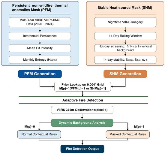
Figure 1. Overview of the PFM/SHM-aware prior-guided contextual fire detection framework.

1.2. Related Work

The evolution of satellite active fire detection has largely centered on refining pixel-level contextual tests. The classic MODIS and VIIRS algorithms employ a combination of absolute thresholds and relative contextual tests to separate fire pixels from their background [5,7,9,24,27]. The VIIRS 375 m algorithm further improves sensitivity to small fires through I-band observations and sensor-specific contextual filtering [5,28]. Nonetheless, long-lived non-wildfire heat sources are often treated as generic thermal anomalies [29], and the baseline logic lacks an explicit mechanism for distinguishing persistent static sources from transient fires using historical persistence information [28,30,31,32].

In parallel, long-term VIIRS/MODIS observations have been used to map persistent heat sources for applications such as gas-flare monitoring, industrial cluster characterization, and emissions inventory development [31,32,33,34,35]. These studies typically produce static masks for industrial or volcanic monitoring; however, such products have not been systematically incorporated as pixel-level priors into the real-time decision logic of operational active fire detection to improve robustness.

Multi-temporal stability analysis also provides discriminative information for separating stable sources from transient events. While geostationary fire products frequently adopt temporal filtering to reduce noise [14,36], and persistence-related considerations have been discussed in the context of polar-orbiting algorithms, operational VIIRS products have not fully exploited multi-day brightness-temperature stability to adapt contextual thresholds for “persistent” versus “normal” pixels within a unified framework. This gap motivates our PFM/SHM-aware parameter-switching design.

1.3. Contributions

By bridging static heat-source screening and dynamic active fire detection, this study makes three contributions: (i) Prior-guided contextual detection via parameter switching. We propose an operationally compatible plug-in layer for a VIIRS 375 m contextual detector that performs pixel-wise parameter switching using spatiotemporal priors, thereby suppressing persistent non-wildfire false alarms without sacrificing sensitivity over non-persistent backgrounds. (ii) We derive a PFM from multi-year VNP14IMG recurrence and stability statistics, providing a reusable prior that targets industrial facilities, gas flares, and volcanic/geothermal hotspots to reduce false positives in routine active fire products. (iii) We develop a multi-day nighttime SHM from VIIRS I4/I5 brightness temperature time series and temporal stability indicators, complementing the PFM by capturing newly established or rapidly intensifying static sources that may be missed by long-term static-source products.

1.4. Paper Organization

Section 2 describes the datasets and study regions and details the construction of PFM and SHM and their integration into the prior-guided contextual detection framework. Section 3 presents quantitative evaluation results across stratified scenarios. Section 4 discusses limitations and potential extensions, and Section 5 concludes the paper.

2. Materials and Methods

2.1. Data and Study Areas

This study employs a multi-source validation framework across diverse geographic regions and fire regimes. The following subsections describe the satellite datasets, auxiliary geospatial layers, and the reference data generation workflow used to evaluate the proposed PFM/SHM-aware detection algorithm.

2.1.1. Satellite Data

Primary data were acquired from the Visible Infrared Imaging Radiometer Suite (VIIRS) onboard the Suomi National Polar-orbiting Partnership (Suomi-NPP) satellite. The data were obtained from the Level-1 and Atmosphere Archive and Distribution System Distributed Active Archive Center (LAADS DAAC) at the National Aeronautics and Space Administration (NASA) Goddard Space Flight Center (Greenbelt, MD, USA). We used three VIIRS products as follows.

VNP02IMG (Collection 2) provides calibrated top-of-atmosphere (TOA) radiances and brightness temperatures for the 375 m imagery (I) bands. We use I4 (3.74 µm) and I5 (11.45 µm) as the primary thermal inputs for anomaly detection and background characterization. VNP03IMG (Collection 2) was used to retrieve observation geometry (solar/sensor zenith angles) and geolocation information, enabling consistent reprojection of multi-day brightness-temperature sequences onto a common fixed grid for temporal stability analysis [5].

The operational active fire product served two purposes: (1) PFM construction: Historical VNP14IMG (Version 2) records (2022–2024) were aggregated to compute pixel-level detection recurrence frequencies, forming the basis of the persistent non-wildfire thermal anomalies mask; (2) Operational product evaluation: The standard product served as the operational benchmark for comparative performance assessment [5].

2.1.2. Auxiliary Datasets

To support scene characterization and result validation, several auxiliary datasets were integrated and resampled to a common grid/projection.

High-resolution optical imagery: Landsat 8/9 Operational Land Imager (OLI) Collection 2 Level-2 images, obtained from the U.S. Geological Survey (USGS), Sioux Falls, SD, USA, and Sentinel-2 Multispectral Instrument (MSI) Level-2A images, provided by the European Space Agency (ESA), Paris, France, were employed for reference (visual) verification, facilitating the visual discrimination of combustion sources from industrial infrastructure [37,38].

Points of interest (POIs): For independent validation of persistent heat sources, we integrated three POI datasets representing major anthropogenic and natural thermal anomaly types: the Global Power Plant Database (GPPD; World Resources Institute, Washington, DC, USA), the ORNL Global Gas Flare Survey derived from VIIRS Night fire (Oak Ridge National Laboratory Distributed Active Archive Center, Oak Ridge National Laboratory, Oak Ridge, TN, USA), and the Smithsonian Institution Global Volcanism Program Holocene Volcanoes database (National Museum of Natural History, Washington, DC, USA), representing power plants, gas flares, and volcanic/geothermal sources, respectively [39,40].

2.1.3. Study Areas

To evaluate algorithmic robustness under varying interference levels, four stratified study-area categories were selected (Table 1).

Table 1. Spatiotemporal information of selected fire and volcanic events.

Event ID	Name	Box	Date Range
1	Cleveland volcanic	(170.05°W–169.85°W, 52.75°N–52.9°N)	2 September 2025
2	Etna volcanic	(14.85°E–15.15°E, 37.65°N–37.85°N)	14 November 2025
3	Sakurajima volcanic	(130.55°E–130.75°E, 31.50°N–31.70°N)	26 November 2025
4	Fuego volcanic	(90.95°W–90.80°W, 14.40°N–14.55°N)	24 October 2025 to 28 October 2025
5	Texas grassland fire	(101.85°W–101.05°W, 35.30°N–35.85°N)	27 February 2024 to 2 March 2024
6	Heilongjiang Crop Fire	(126.95°E–127.30°E, 46°N–46.8°N)	25 October 2025 to 26 October 2025

(i)

Industrial/urban regions: Regions dominated by heavy industry and intense urbanization. These are used to assess the algorithm’s ability to suppress false alarms caused by persistent non-fire heat sources and urban heat islands.

(ii)

Volcanic/geothermal regions: Areas dominated by persistent natural thermal anomalies (e.g., active craters and geothermal fields). These regions are used to evaluate suppression of non-wildfire geological hotspots while retaining sensitivity to dynamic events such as lava flows extending beyond historical anomaly footprints.

(iii)

Agricultural burning regions: Areas characterized by seasonal crop residue burning. These scenarios test the algorithm’s sensitivity to small-scale, fragmented, and transient fires that often coexist with human settlements.

(iv)

Forest/grassland fire regions: Relatively homogeneous landscapes prone to natural wildfires. These areas establish an operational product for evaluating detection rates (recall) and capturing the spatiotemporal evolution of large-scale fire events.

2.1.4. Reference Data Construction

Reference labels were generated on Google Earth Engine (Google LLC, Mountain View, CA, USA; web-based platform available at https://earthengine.google.com/ (accessed on 29 December 2025)) by co-locating each VIIRS 375 m candidate pixel with the nearest cloud-free Sentinel-2 MSI or Landsat 8/9 OLI observation acquired within ±1 day after the overpass (for nighttime overpasses, we used the nearest subsequent daytime optical acquisition within 1 day after the overpass). Cloud and cloud shadows were removed using the official QA layers (Sentinel-2 QA60/SCL; Landsat QA_PIXEL). To ensure reproducibility, strictly defined labeling criteria were applied. A candidate was classified as a confirmed fire only if it satisfied one of the following conditions: (1) the distinct presence of smoke plumes or active flaming fronts; or (2) a visible fresh burn scar corroborated by a temporal drop in the Normalized Burn Ratio ($\Delta NBR\ge 0.10$). Conversely, candidates were labeled as uncertain if visual attribution was ambiguous (e.g., distinguishing faint smoke from thin cloud/haze) or if thermal anomalies lacked a corresponding optical footprint due to sub-pixel scale limits. Each candidate pixel was independently labeled by two analysts following the criteria above. Disagreements were resolved through consensus review. Samples that remained in the “Uncertain” category after review were excluded from quantitative evaluation. In total, 565 uncertain cases were removed from 4000 candidates, resulting in a final evaluation dataset of N = 3435 samples.

2.2. Methodology

As illustrated in Figure 1, Section 2.2.1 and Section 2.2.2 describe the construction of PFM and SHM, while Section 2.2.3 and Section 2.2.4 present the prior-aware threshold-switching strategy integrated into a contextual detector.

2.2.1. Construction of PFM

The PFM is constructed from VNP14IMG using a continuous 3-year window from 2022 to 2024 (K = 3). We apply strict product-level quality control: cloud-contaminated or invalid detections are removed, and only records with reliable radiometric and geometric quality flags are retained.

All statistics are computed on a fixed 0.004° WGS84 latitude–longitude land grid. Each valid detection is assigned to the nearest grid cell using the pixel-center geolocation. To avoid double counting, detections are aggregated by UTC-day: for a grid cell $i$, a day contributes one hit if at least one detection occurs on that day.

Activity and persistence definitions: Let $N_{\mathrm{hits}}\left(i\right)$ denote the total number of hit-days during 2022–2024 and let $N_{\mathrm{h}\mathrm{i}\mathrm{t}\mathrm{s},y}\left(i\right)$ denote the hit-days in year $y$. We define the number of active years $N_{\mathrm{y}\mathrm{e}\mathrm{a}\mathrm{r}\mathrm{s}}\left(i\right)$ using a within-year reliability criterion. Specifically, a year is counted as active if $N_{\mathrm{h}\mathrm{i}\mathrm{t}\mathrm{s},y}\left(i\right)\ge 10$. Based on these metrics, we define the interannual persistence and mean annual hit intensity as follows:

$$f_{year}\left(i\right)={\displaystyle \frac{N_{\mathrm{years}}\left(i\right)}{K}},$$

(1)

$$\overline{h}\left(i\right)={\displaystyle \frac{N_{\mathrm{hits}}\left(i\right)}{K}}.$$

(2)

Here, $f_{year}\left(i\right)$ denotes interannual recurrence and $\overline{h}\left(i\right)$ reflects long-term activity intensity. Grid cells with $N_{\mathrm{years}}\left(i\right)=0$ are classified as non-candidates and removed from further processing.

High recurrence can also arise from strongly seasonal agricultural burning. To distinguish genuine persistent heat sources (e.g., gas flares, industrial complexes, and volcanoes) from seasonal events, we quantify seasonality using normalized month-of-year entropy. Let $n_m\left(i\right)$ denote the number of hit-days in month $m\in \left\{1,\dots ,12\right\}$ summed over 2022–2024. We define:

$$p_m\left(i\right)=n_m\left(i\right)/{\sum }_{m=1}^{12}{n}_m\left(i\right),$$

(3)

and the normalized entropy as:

$$H_{\mathrm{norm}}(i)={\displaystyle \frac{-\sum _{m=1}^{12}{p}_m(i)\mathrm{l}\mathrm{n}{p}_m(i)}{\ln 12}},H_{\mathrm{norm}}(i)\in [0,1].$$

(4)

Persistent non-wildfire sources are typically more month-uniform (higher $H_{\mathrm{norm}}$), whereas seasonal burning is month-concentrated (lower $H_{\mathrm{norm}}$). To ensure statistical stability, $H_{\mathrm{norm}}\left(i\right)$ is computed only for cells with $N_{\mathrm{hits}}\left(i\right)\ge 15$.

A grid cell $i$ is included in the $K=3$ main PFM when it satisfies:

$$f_{\mathrm{years}}\left(i\right)\ge f_{years}^{min}\wedge \overline{h}\left(i\right)\ge {\overline{h}}^{\mathrm{m}\mathrm{i}\mathrm{n}}\wedge H_{\mathrm{norm}}(i)\ge H^{min},$$

(5)

We adopt a conservative persistence default $f_{\mathrm{y}\mathrm{e}\mathrm{a}\mathrm{r}\mathrm{s}}^{\mathrm{m}\mathrm{i}\mathrm{n}}=2/3$ (active in at least 2 out of 3 years). The intensity threshold ${\overline{h}}^{\mathrm{m}\mathrm{i}\mathrm{n}}$ is set to the 60th percentile and entropy threshold $H^{min}=0.60$; both are calibrated to suppress seasonal noise (Section 2.2.4).

The $K=3$ prior is high precision but can miss stable sources that emerge only in the most recent year. A source appearing only in 2024 yields $f_{\mathrm{year}}=1/3$, which fails the recurrence criterion regardless of its within-year stability. We therefore build a 2024-only complement mask, ${PFM}_{\mathrm{K}1}$, using a within-year hit threshold:

$${PFM}_{\mathrm{K}1}\left(i\right)=1\left[N_{hits}^{2024}\left(i\right)\ge T\right],$$

(6)

We set $T=30$ to balance retention of stable new sources against transient candidates. The final mask is:

$${PFM}_{\mathrm{final}}\left(i\right)={PFM}_{K3}\left(i\right)\vee {PFM}_{K1}\left(i\right),$$

(7)

For reproducibility, we store a source label for each masked cell (K3-only, K1-only, or overlap). Density comparisons (Figure 2) show that the $K=1$ mask largely follows the spatial pattern of the main $K=3$ PFM, while K1-only pixels form geographically coherent clusters rather than random speckles. This spatial coherence supports the need for a latest-year complement.

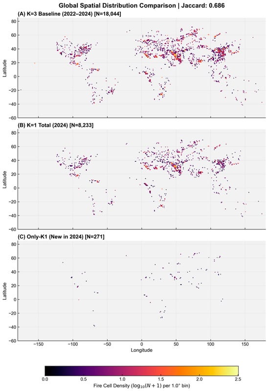
Figure 2. Spatiotemporal comparison of PFM: (A) K = 3 baseline (2022–2024); (B) K = 1 annual PFM (2024); and (C) newly detected PFM grid cells in 2024 relative to the baseline.

To account for geolocation uncertainty and the spatial extent of point-source emissions, we apply two morphological steps to the binary mask: (i) dilation with radius of 1 grid cell, and (ii) 4-neighbor connected-component filtering with a minimum cluster size $A_{\mathrm{m}\mathrm{i}\mathrm{n}}=2$ cells. The resulting PFM serves as a robust static prior. To prevent temporal leakage, we adopt a causal (rolling) design: for validation events in 2024, the PFM uses data up to 2023, whereas, for validation events in 2025, it uses the full 2022–2024 window. All reported results follow this rule unless stated otherwise.

2.2.2. Construction of SHM

However, the annually updated PFM can be slow to reflect new or rapidly intensifying heat sources. To address this limitation, we construct an SHM from nighttime VIIRS brightness-temperature time series. Nighttime observations are selected using the product day/night flag, which reduces solar contamination and suppresses diurnal variability, yielding a smoother background for identifying persistent static thermal anomalies.

The SHM follows a “high-SNR single-pass detection + temporal accumulation” design: we screen anomalies on each nighttime overpass and then accumulate detections over multiple days. This strategy reduces the reliance on long-term recurrence while enabling timely updates for newly emerging static heat sources.

Per-overpass adaptive anomaly detection. For each nighttime overpass, we retrieve the VIIRS I4 and I5 brightness temperatures, $T_4$ and $T_5$, and compute the inter-band difference:

$$\mathsf{\Delta }{T}_{45}=T_4-T_5.$$

(8)

Using a sliding window centered at each pixel, we compute local background mean and standard deviation for $\mathsf{\Delta }{T}_{45}$ ($\overline{∆T_{45}}$ and ${\sigma }_{\mathsf{\Delta }}$), and for $T_4$ (${\bar{T}}_{b4}$ and ${\sigma }_{T4}$). A pixel is flagged as candidate if it satisfies the following dual-constraint condition:

$$\mathsf{\Delta }{T}_{45}\ge \max \left(\overline{∆T_{45}}+\alpha {\sigma }_{\mathsf{\Delta }},\overline{∆T_{45}}+{\mathsf{\Delta }}_{abs}\right)\wedge T_4\ge \max \left({\overline{T}}_{b4}+\beta {\sigma }_{T4},T_4^{min}\right).$$

(9)

Here, $\alpha$ controls the statistical significance threshold, $\beta$ is the thermal anomaly scaling factor, ${\mathsf{\Delta }}_{\mathrm{abs}}$ enforces a minimum absolute inter-band contrast, and $T_4^{\mathrm{m}\mathrm{i}\mathrm{n}}$ is an absolute high-temperature floor. We adopt calibrated baseline settings (e.g., $\alpha =2.0$, Section 2.2.4).

Spatiotemporal aggregation and decision rule. Per-overpass hot-pixel flags are mapped to a fixed 0.004° grid via nearest-neighbor assignment and de-duplication by UTC-day: if any nighttime overpass triggers Equation (9) for a given grid cell, that day is counted once as a “hot day”. Over a rolling window of $N_d=14$ days, we define $N_{hot}\left(i\right)$ as the number of hot days for grid cell $i$. A cell is labeled as a short-term heat source, ($SHM=1$), if $N_{\mathrm{h}\mathrm{o}\mathrm{t}}\ge 1$, to prioritize timeliness for newly emerging or intensifying static sources. The nighttime-only constraint and significance-based screening in Equation (9) help limit accidental activations.

Handling prolonged data gaps. We use a fixed calendar window ($N_d=14)$ to enforce time decay so inactive sources expire naturally. Although persistent cloud cover may cause temporary expiration, the $H_{min}=1$ rule re-activates the source upon the first subsequent clear-sky re-detection, limiting potential rebounds in commission errors to a short interval (typically a single overpass).

Limitations of SHM. Short-term nighttime stability is not unique to non-wildfire heat sources; some anthropogenic burning may also appear stable and trigger SHM. SHM does not hard-mask detections: it only switches the detector to a stricter parameter set. In our evaluation dataset, SHM was not activated for true-fire subsets, but this failure mode remains possible and should be examined in targeted case studies.

2.2.3. PFM/SHM-Aware Contextual Detection Framework

The proposed method is a lightweight spatiotemporal prior layer superimposed on a VNP14-style contextual detector. It preserves standard preprocessing (e.g., calibration and geolocation) and modifies only pixel-level parameter selection via prior-aware switching. Each VIIRS 375 m pixel is mapped to its nearest 0.004° grid cell. The “VNP14-style baseline” refers to our in-house implementation under the Normal parameter set, whereas the proposed method switches to the Masked set for pixels flagged by the PFM/SHM priors; all other contextual-test steps (Equations (10)–(13)) remain unchanged. Pseudo-code is provided in Supplementary Algorithm S1.

For each observation pixel $p$, we define a prior flag $M\left(p\right)$: $M\left(p\right)=1$ if either prior is active for the corresponding grid cell ($PFM\left(p\right)=1$ or $SHM\left(p\right)=1$), and $M\left(p\right)=0$ otherwise. We apply the baseline contextual tests with the Normal parameter set when $M\left(p\right)=0$, and switch to the Masked parameter set when $M\left(p\right)=1$.

Prior-aware candidate screening. Standard validity masking excludes clouds, water bodies, and low-quality data. Valid pixels are screened as potential fire candidates using mode-dependent thresholds:

$$C\left(p\right)=1\left(T_4\right(p)\ge T_{4,min}^{D\left(p\right)}\left(M\left(p\right))\wedge \mathsf{\Delta }{T}_{45}(p)\ge (\mathsf{\Delta }{T}_{45}{)}_{\mathrm{m}\mathrm{i}\mathrm{n}}\left(M\left(p\right)\right)\right),$$

(10)

Here, $D\left(p\right)\in \{\mathrm{day},\mathrm{night}\}$. The thresholds $T_{4,\mathrm{m}\mathrm{i}\mathrm{n}}^{day}\left(M\right)$, $T_{4,\mathrm{m}\mathrm{i}\mathrm{n}}^{night}\left(M\right)$, and $(\mathsf{\Delta }{T}_{45}{)}_{\mathrm{m}\mathrm{i}\mathrm{n}}\left(M\right)$ are determined by the mask status $M\left(p\right)$ and mode $D\left(p\right)$. Only pixels satisfying $C\left(p\right)=1$ proceed to the contextual background characterization.

Dynamic background characterization. For each candidate $p$, we expand an adaptive background window $W$, from $W_0$ to $W_{max}$ until:

$$\mid {\mathsf{\Omega }}_{bg}(p,W)\mid \ge N_{bg}^{min},$$

(11)

${\mathsf{\Omega }}_{bg}(p,W)$ excludes the candidate pixel, cloud/water/invalid pixels, other candidates (to avoid mutual contamination), and obvious noise outliers. Over ${\mathsf{\Omega }}_{bg}(p,W)$, we compute $\overline{∆T_{45}}\left(p\right)$, ${\sigma }_{\mathsf{\Delta }}\left(p\right)$, ${\overline{T}}_{b4}\left(p\right)$, and ${\sigma }_{T4}\left(p\right)$.

Contextual confirmation (day/night rules). A candidate is confirmed as fire only if its thermal signal significantly exceeds the local background:

Daytime:

$$\begin{gathered} ∆T\_45\left(p\right)\ge max(¯(∆T\_45\left)\right(p)+a\_day(M\left(p\right))\sigma \_\Delta (p),¯(∆T\_45\left)\right(p)+∆\_abs^day(M\left(p\right)\left)\right) \\ \wedge T_4\left(p\right)\ge \mathrm{m}\mathrm{a}\mathrm{x}\left({\overline{T}}_{b4}\left(p\right)+b_{day}\left(M\left(p\right)\right){\sigma }_{T4}\left(p\right),T_{4,min}^{day}\left(M\left(p\right)\right)\right), \end{gathered}$$

(12)

Nighttime:

$$\begin{gathered} ∆T_{45}\left(p\right)\ge \max \left(\overline{∆T_{45}}\left(p\right)+a_{night}\left(M\left(p\right)\right){\sigma }_{\mathsf{\Delta }}\left(p\right),\overline{∆T_{45}}\left(p\right)+{∆}_{abs}^{night}\left(M\left(p\right)\right)\right) \\ \wedge T_4\left(p\right)\ge \mathrm{m}\mathrm{a}\mathrm{x}\left({\overline{T}}_{b4}\left(p\right)+b_{night}\left(M\left(p\right)\right){\sigma }_{T4}\left(p\right),T_{4,min}^{night}\left(M\left(p\right)\right)\right), \end{gathered}$$

(13)

Here, $a(\cdot )$ and $b(\cdot )$ are standard-deviation multipliers controlling the required contextual contrast for $\mathsf{\Delta }{T}_{45}$ and $T_4$, respectively, while ${\mathsf{\Delta }}_{abs}(\cdot )$ and $T_{4,\mathrm{m}\mathrm{i}\mathrm{n}}(\cdot )$ impose absolute lower bounds. A pixel is reported as a fire detection when the corresponding day/night test is satisfied:

$$F\left(p\right)=1\left\{{\mathsf{\Phi }}_{D\left(p\right)}\right(p)=\mathrm{t}\mathrm{r}\mathrm{u}\mathrm{e}\},$$

(14)

The Masked parameter set uses higher $a(\cdot )$, $b(\cdot )$, ${\mathsf{\Delta }}_{abs}(\cdot )$, and $T_{4,\mathrm{m}\mathrm{i}\mathrm{n}}(\cdot )$ values to reduce repeated triggering over persistent non-wildfire sources; this stricter logic is applied only when $M\left(p\right)=1$. Otherwise, $M\left(p\right)=0$ and the detector reverts to the Normal (baseline) configuration.

2.2.4. Parameterization and Calibration

This section calibrates key thresholds for PFM/SHM and motivates the Masked parameter set.

Calibration of PFM thresholds. To build a robust PFM, we calibrate three thresholds from the candidate set defined by $f_{\mathrm{y}\mathrm{e}\mathrm{a}\mathrm{r}\mathrm{s}}\ge 2/3$. For the 2024-only complement (${PFM}_{K1}$), we set the within-year stability threshold to $T=30$ (Figure 3), balancing retention of stable new sources against transient noise.

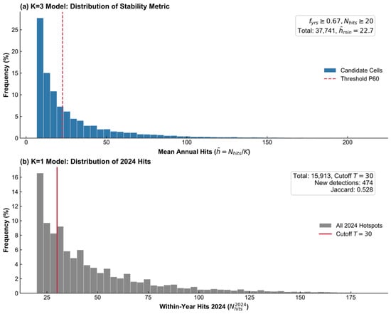
Figure 3. Threshold calibration and motivation for the latest-year complement: (a) $\overline{h}={\displaystyle \frac{N_{\mathrm{h}\mathrm{i}\mathrm{t}\mathrm{s}}}{K}}$ for K = 3 and the (P60); (b) $N_{\mathrm{h}\mathrm{i}\mathrm{t}\mathrm{s}}^{2024}$ for $K=1$ and $T=30$.

To suppress strongly seasonal agricultural burning, we set the entropy gate to $H^{\mathrm{m}\mathrm{i}\mathrm{n}}=0.60$. For a uniform distribution across $M$ effective months, $H_{\mathrm{n}\mathrm{o}\mathrm{r}\mathrm{m}}=\mathrm{l}\mathrm{n}M/\mathrm{l}\mathrm{n}12$. Thus, $H^{\mathrm{m}\mathrm{i}\mathrm{n}}=0.60$ roughly corresponds to retaining sources active for $M\approx {12}^{0.60}\approx 4.4$ months or more. As shown in Figure 4, this entropy gate has negligible impact under conservative ${\overline{h}}^{\mathrm{m}\mathrm{i}\mathrm{n}}$ choices but becomes increasingly important when ${\overline{h}}^{\mathrm{m}\mathrm{i}\mathrm{n}}$ is relaxed, acting as a safeguard against seasonal artifacts.

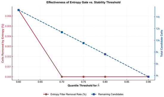
Figure 4. Entropy-gate effectiveness versus the quantile used for ${\overline{h}}^{\mathrm{m}\mathrm{i}\mathrm{n}}$.

We then set the mean annual intensity threshold ${\overline{h}}^{\mathrm{m}\mathrm{i}\mathrm{n}}$ to the P60 quantile of the $\overline{h}$ distribution (Figure 3a), which removes sporadic noise while preserving persistent activity.

Sensitivity analysis of PFM design parameters. We perform a one-at-a-time sensitivity analysis around the default configuration ($N_{hit,y}\ge 10$, ${\overline{h}}_{\mathrm{m}\mathrm{i}\mathrm{n}}=$ P60, $H_{\mathrm{m}\mathrm{i}\mathrm{n}}=0.60$, dilation radius $r=1$, and minimum connected-component size $s=2$). For each setting, we rebuild the PFM from the same 2022–2024 recurrence database and summarize (i) mask size $N_{\mathrm{f}\mathrm{i}\mathrm{n}\mathrm{a}\mathrm{l}}$ and (ii) similarity to the default mask using the Jaccard index (Table S1). Results show that $H_{\mathrm{m}\mathrm{i}\mathrm{n}}$ and $s$ are largely insensitive within practical ranges, but dominate spatial expansion; therefore, we fix $r=1$ and $s=2$ in subsequent experiments.

Sensitivity analysis of SHM parameters. For SHM, we test the robustness of the adaptive threshold over a representative East Asian sub-region. Increasing $\alpha$ from 1.5 to 2.0 yields essentially unchanged precision/recall, and even $\alpha =4.0$ retains ~88% of detections (Figure 5). We therefore use $\alpha =2.0$ as a stable operational baseline.

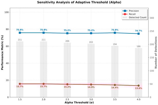
Figure 5. Sensitivity of the SHM adaptive threshold $\alpha$ on detection performance.

We also examine temporal accumulation from 9 September to 6 October 2024. Extending the window from 1 to 14 days steadily recovers valid heat sources (newly added detections increase from ~2% to ~19%) while maintaining high confidence (>70%) (Figure 6), supporting $N_d=14$.

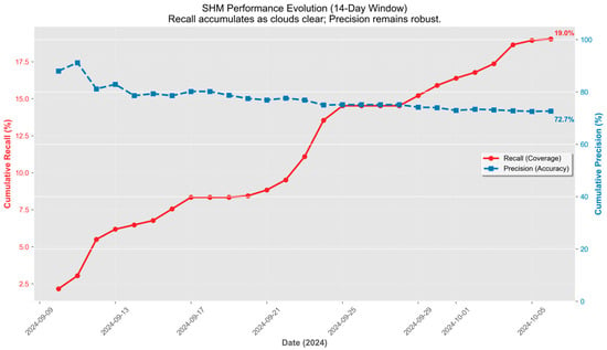
Figure 6. Temporal accumulation trends of SHM detection.

Finally, we compare the default inclusion rule $H_{min}=1$ with a stricter alternative $H_{min}=2$ (Table 2). Although $H_{min}=2$ reduces SHM-only cells by 78.4%, it substantially reduces the recall proxy (PFM coverage) from 15.7% to 6.6%. Table 3 further shows that most single-hit cells ($N_{hot}=1$) remain PFM-consistent (69.9%), indicating that sparsity does not imply low quality. We thus retain $H_{min}=1$ to prioritize timely identification of emerging sources.

Table 2. Robustness of SHM to $H_{min}$ (fixed $N_d=14$).

${\mathit{H}}_{\mathit{m}\mathit{i}\mathit{n}}$	SHM Cells	$\mathit{P}\mathit{F}\mathit{M}\cap \mathit{S}\mathit{H}\mathit{M}$	SHM-Only	Precision Proxy (%)	Recall Proxy (%)
1	211	160	51	75.83	15.7
2	78	67	11	85.90	6.58

Table 3. Distribution of $N_{hot}$ (window end: 6 October 2024).

${\mathit{N}}_{\mathit{h}\mathit{o}\mathit{t}}$	SHM Cells	Share of SHM (%)	$\mathit{P}\mathit{F}\mathit{M}\cap \mathit{S}\mathit{H}\mathit{M}$	SHM-Only	SHM-Only Within Bin (%)
1	133	63.0	93	40	30.1
2	49	23.2	39	10	20.4
3	11	5.2	11	0	0.0
4	11	5.2	10	1	9.1
5	5	2.4	5	0	0.0
6	2	0.9	2	0	0.0
Total	211	100.0	160	51	-

Note: SHM-only is used as an upper-bound proxy of false alarms, acknowledging that some may be newly emerging static sources absent from PFM.

Masked-mode threshold adaptation. To calibrate thresholds for the Masked parameter set, we analyze an industrial ROI (110°E–112°E, 34°N–36°N). Mask-covered pixels ($M=1$) show systematically lower upper-tail anomaly indicators than unmasked pixels ($M=0$) (Figure 7 and Figure 8). During daytime, $\mathsf{\Delta }{T}_{45}$ decreases by 11.7–15.7 K at P95–P99, indicating that a single global threshold would produce excessive commission errors over persistent hotspots.

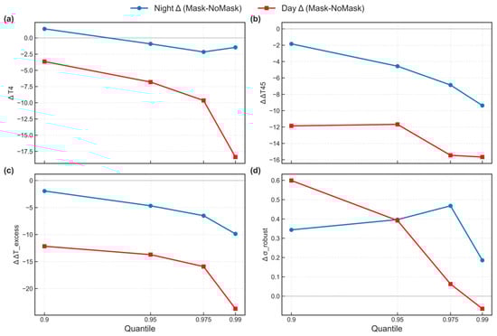
Figure 7. Quantile differences $\mathsf{\Delta }q=q_{M=1}-q_{M=0}$ in the ROI (day/night), evaluated at quantiles 0.90, 0.95, 0.975, and 0.99. Panels show (a) $T_4$, (b) $\mathsf{\Delta }{T}_{45}$, (c) $\mathsf{\Delta }{T}_{\mathrm{excess}}=\mathsf{\Delta }{T}_{45}-\overline{∆T_{45}}$, and (d) ${\sigma }_{\mathrm{robust}}$ (robust background dispersion). Negative $\mathsf{\Delta }q$ indicates a downward shift within the mask.

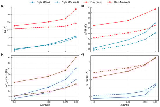
Figure 8. Quantile curves (0.90–0.99) of (a) $T_4$, (b) $\mathsf{\Delta }{T}_{45}$, (c) $\mathsf{\Delta }{T}_{\mathrm{excess}}$, and (d) ${\sigma }_{\mathrm{robust}}$, stratified by day/night and mask membership (solid: $M=0$; dashed: $M=1$).

Within the ROI, $\mathsf{\Delta }T$-based indicators are consistently suppressed in the masked population, with a larger separation during daytime (Figure 7). At P95–P99, $T_4$ decreases by 6.8–18.4 K, $\mathsf{\Delta }{T}_{45}$ by 11.7–15.7 K, and $\mathsf{\Delta }{T}_{\mathrm{excess}}$ by 13.7–23.7 (K relative to $M=0$). At night, the same pattern persists but is weaker (e.g., $\mathsf{\Delta }{T}_{45}$ drops from −4.6 K at P95 to −9.4 K at P99). In contrast, ${\sigma }_{\mathrm{robust}}$ changes only modestly (typically within ±0.6 K), suggesting the separation is driven mainly by reduced anomaly strength rather than background dispersion.

A threshold scan shows that increasing $T_4$ monotonically increases suppression at the cost of retention (Figure 9). We select 335 K/315 K near the elbow, achieving suppression 0.828 while retaining 1802 candidates out of $N_{\mathrm{base}}=\mathrm{10,455}$. More aggressive settings (e.g., 340 K/320 K) yield higher suppression (~0.918) but much lower retention (855), whereas looser settings (e.g., 330 K/310 K) retain more candidates (3721) with limited suppression (0.645). Final Normal and Masked configurations are summarized in Table 4.

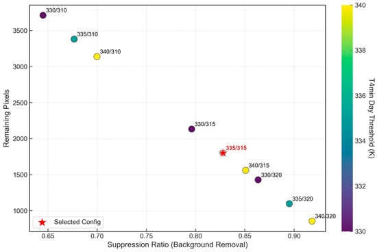
Figure 9. Suppression–retention trade-off of strengthened within-mask thresholds in the ROI $\left(a_{day}=4.0,a_{night}=4.5\right)$. $\mathrm{Suppression}=1-N_{\mathrm{keep}}/N_{\mathrm{base}}$, where $N_{\mathrm{base}}$ is the within-mask candidate count under the baseline and $N_{\mathrm{keep}}$ is the retained count after strengthening. Each point corresponds to a $\left(T_{4,\mathrm{m}\mathrm{i}\mathrm{n}}^{\mathrm{day}},T_{4,\mathrm{m}\mathrm{i}\mathrm{n}}^{\mathrm{night}}\right)$ pair, and the red star marks the selected setting (335 K/315 K).

Table 4. Normal/Masked parameter configuration under PFM/SHM constraints.

Category	Parameter	Symbol	Normal $\mathit{M}=0$	Masked $\mathit{M}=1$
$\mathrm{Daytime}∆T_{45}$ contrast	$\mathrm{SD}\mathrm{multiplier}\alpha$	${\alpha }_{day}$	2.0	4.0
$\mathrm{Nighttime}∆T_{45}$ contrast	$\mathrm{SD}\mathrm{multiplier}\alpha$	${\alpha }_{night}$	3.0	4.5
$\mathrm{Daytime}{T}_4$ contrast	$\mathrm{SD}\mathrm{multiplier}\beta$	${\beta }_{day}$	3.0	4.5
$\mathrm{Nighttime}{T}_4$ contrast	$\mathrm{SD}\mathrm{multiplier}\beta$	${\beta }_{night}$	3.0	4.5
$\mathrm{Daytime}\mathrm{absolute}\mathsf{\Delta }$ bound	absolute increment	${∆}_{abs}^{day}$	10 K	10 K
$\mathrm{Nighttime}\mathrm{absolute}\mathsf{\Delta }$ bound	absolute increment	${∆}_{abs}^{night}$	10 K	10 K
$\mathrm{Daytime}\mathrm{absolute}{T}_4$ bound	absolute threshold	$T_{4,min}^{day}$	325 K	335 K
$\mathrm{Nighttime}\mathrm{absolute}{T}_4$ bound	absolute threshold	$T_{4,min}^{night}$	300 K	315 K

3. Results

3.1. Validation of the PFM via Multi-Source POI Analysis

3.1.1. Multi-Source POI Datasets

To independently validate the PFM, we used three point-of-interest (POI) datasets representing common persistent heat sources: GPPD power plants, VIIRS gas flares, and Holocene volcanoes/geothermal sites. These datasets correspond to major anthropogenic and natural thermal anomaly types, including thermal/geothermal facilities, gas flares, and volcanic or geothermal sources. They were used as external references to assess whether the PFM (a) covers known persistent heat sources and (b) spatially aligns with plausible heat-source locations.

3.1.2. Evaluation Metrics

We use a two-way validation strategy with symmetric distance thresholds. We set the POI buffer radius equal to the association distance $R$ and test $r=R\in \{2,5,10\}$ km.

POI coverage rate ($H_{POI}$). For each POI, we create a buffer of radius $r$. If the buffer intersects at least one PFM pixel, the POI is counted as a hit. Let $N_{POI}$ be the total number of POIs and $N_{hit}$ the number of hit POIs:

$$H_{POI}={\displaystyle \frac{N_{hit}}{N_{POI}}}\times 100\%,$$

(15)

PFM attribution rate ($A_{PFM}$). We represent each connected PFM polygon by its centroid and compute the Euclidean distance $d$ to the nearest POI of a given class. If $d\le R$, the polygon is considered associated with that POI class. Let $M$ be the number of PFM polygons and $M_{\mathrm{n}\mathrm{e}\mathrm{a}\mathrm{r}}$ the number satisfying the distance constraint:

$$A_{\mathrm{P}\mathrm{F}\mathrm{M}}={\displaystyle \frac{M_{\mathrm{n}\mathrm{e}\mathrm{a}\mathrm{r}}}{M}}\times 100\%,$$

(16)

Together, $H_{POI}$ answers “what fraction of known POIs are covered by the PFM”, whereas $A_{PFM}$ answers “what fraction of PFM regions can be attributed to typical persistent heat sources in existing databases”.

3.1.3. Quantitative Results Under a Strict Threshold ($r=R=2\mathrm{k}\mathrm{m}$)

Table 5 summarizes results for each POI class and their union at km. Gas flares show the strongest agreement with the PFM (highest $H_{POI}$ and $A_{\mathrm{P}\mathrm{F}\mathrm{M}}$), consistent with their persistent high-temperature emissions. In contrast, Holocene volcanoes exhibit low matching rates because the catalog includes many dormant or weakly active systems that do not produce persistent VIIRS-detectable thermal signals. For the union of POI categories, 47.49% of PFM polygons are associated with at least one POI type within 2 km, indicating that nearly half of the PFM regions align with recorded persistent heat sources under strict proximity constraints.

Table 5. Validation results of PFM persistent fires based on three POI categories ($r=R=2\mathrm{k}\mathrm{m}$).

POI Type	Number of POIs	Hit Rate $({\mathit{H}}_{\mathbf{P}\mathbf{O}\mathbf{I}}$)	$\mathbf{Consistency}({\mathit{A}}_{\mathbf{P}\mathbf{F}\mathbf{M}}$)
GPPD Thermal + Geothermal	9905	4.78%	10.06%
VIIRS Gas Flare Sites	18,695	13.40%	38.89%
Holocene Volcanoes/Geothermal	1422	2.32%	1.16%
Union of Three POI Types	30,022	10.03%	47.49%

3.1.4. Sensitivity Analysis of Spatial Thresholds

Relaxing the spatial threshold from 2 km to 5 km and 10 km increases both $H_{\mathrm{P}\mathrm{O}\mathrm{I}}$ and $A_{\mathrm{P}\mathrm{F}\mathrm{M}}$ (Figure 10). Power plants show a marked rise in agreement as $R$ increases (10.06% → 20.39% → 29.36%), consistent with geolocation mismatches between facility coordinates and detected heat-source clusters. Gas flares remain the strongest correlation with the PFM (38.89% → 42.79% → 45.59%). For the union of POI classes, 65.88% of PFM polygons are associated with at least one POI type at $R=10$ km, suggesting that roughly two-thirds of PFM regions lie within the neighborhood of recorded persistent heat sources.

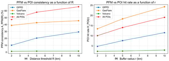
Figure 10. PFM validation versus spatial threshold (2–10 km): (a) PFM Consistency $A_{\mathrm{P}\mathrm{F}\mathrm{M}}$ vs. distance threshold $R$; (b) POI Hit Rate $H_{\mathrm{P}\mathrm{O}\mathrm{I}}$ vs. buffer radius $r$. Thresholds increase from 2 km to 10 km. Gas flares show the strongest explanatory power; the union of POI types explains ~65.88% of PFM regions at $R=10$ km.

3.1.5. Discussion and Limitations

POI-based validation measures spatial overlap between the PFM and recorded persistent heat sources, but unmatched PFM regions should not be interpreted as false positives. Incomplete matching likely reflects (i) limited coverage of POI databases for small-to-medium industrial sites (e.g., brick kilns, informal smelting, waste burning), (ii) heterogeneous thermal behavior (some facilities exhibit weak or intermittent thermal signals), and (iii) the complementary value of the PFM in revealing persistent heat-source clusters not explicitly annotated in common databases. Overall, the POI analysis supports the PFM as a meaningful prior for suppressing persistent non-wildfire thermal anomalies in active fire detection.

3.2. Reliability and Robustness of the Proposed Framework

Section 3.1 validates the spatial plausibility of the PFM prior. We next evaluate whether the PFM/SHM-aware framework remains reliable in challenging cases, focusing on (i) avoiding over-suppression during extreme industrial accidents, (ii) handling diverse volcanic environments, and (iii) adapting to newly emerged (“cold-start”) industrial heat sources.

3.2.1. Robustness Under Extreme Industrial Accident Events

To assess omission risk under extreme conditions, we analyze nighttime $T_4$ time series at the Balongan around the 29 March 2021 explosion (Figure 11). During normal operations (7–28 March), peak $T_4$ values (260–306 K) remain below the strict masked-mode threshold (~315 K), resulting in suppression of routine emissions and zero false alarms. On the explosion night (29 March), $T_4$ surges to 339.3 K, exceeds the threshold, and triggers a detection. This case shows that the framework suppresses routine industrial heat while remaining responsive to sudden high-energy events, reducing the over-suppression risk associated with purely static masking.

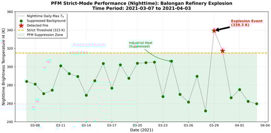
Figure 11. Nighttime VIIRS I4 brightness temperature ($T_4$) at the Balongan refinery before and after the explosion on 29 March 2021. Nighttime observations are used to reduce solar-glint interference and ensure stable monitoring.

3.2.2. Adaptability to Complex Volcanic Scenarios

Persistent geothermal signals near volcanic craters can cause non-wildfire interference in operational fire products. We compare VNP14IMG and the proposed method over four representative volcanoes (Figure 12). For Etna and Sakurajima, VNP14IMG exhibits persistent crater-centered detections that are undesirable for wildfire monitoring; the proposed method suppresses these static signals using the PFM prior. Near-coincident Sentinel-2 imagery confirms no fresh burn scars, and cross-checks with independent fire products indicate no wildfire records in the vicinity on those dates. For Fuego, a lava flow extends beyond the prior boundary; the proposed method detects this expanding anomaly, indicating sensitivity to dynamic growth rather than indiscriminate suppression. For Cleveland, persistent cloud cover limits robust PFM construction; in this data-scarce setting, the method behaves conservatively and remains sensitive, producing results consistent with VNP14IMG to avoid omission.

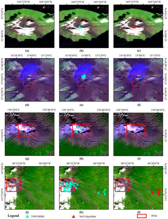
Figure 12. Thermal anomaly detection maps for four representative volcanic regions. (a,d,g,j) VNP14IMG detections; (b,e,h,k) detections from the proposed method; (c,f,i,l) detection difference maps. Rows 1–4 correspond to Cleveland, Etna, Sakurajima, and Fuego volcanoes, respectively.

3.2.3. SHM-Triggered Stabilization for Newly Emerged Industrial Heat Sources (“Cold Start”)

Because the PFM is updated on annual or multi-year cycles, it can lag newly commissioned or rapidly intensifying industrial heat sources, creating a cold-start window without long-term prior coverage. We illustrate this using a newly emerged gas flare in the Permian Basin (4–18 February 2023; Figure 13).

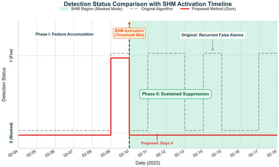
Figure 13. Cold-start example for a newly established industrial heat source in the Permian Basin (31.162°N, 103.614°W). The dashed line marks 10 February 2023, when the SHM activation threshold is first met. Left: Phase I (evidence accumulation, 4–9 February); Right: Phase II (SHM activation and sustained suppression, from 10 February).

During Phase I (4–9 February; 13 nighttime overpasses), the source lies outside the historical PFM footprint and the SHM has not yet accumulated sufficient evidence within the rolling window. The framework therefore follows the baseline logic, and detections may occur (Status = 1). On 10 February (vertical dashed line), the accumulated nighttime evidence first satisfies the SHM activation criterion, switching the pixel to the stricter masked-mode logic and enabling sustained suppression of recurrent non-fire detections from the newly established flare (Status = 0). In contrast, the baseline algorithm continues to produce intermittent false alarms. This example shows that SHM provides a timely pathway from “detect as anomaly” to “recognize as stable heat source and suppress,” without waiting for the next PFM update.

3.3. Evaluation of True Fire Detection

The above analyses focus on suppressing persistent non-wildfire anomalies. We next verify that the proposed framework preserves detection capability for true fires and improves sensitivity to weak and fragmented targets.

3.3.1. Forest and Grassland Fires

In major combustion zones, the proposed detections closely match baseline clusters, indicating stable performance for high-intensity fires (Figure 14). Near fire edges, the baseline sometimes produces isolated detections over unburned areas; visual checks with near-coincident high-resolution imagery suggest these are commission errors caused by complex backgrounds. The proposed method suppresses these spurious pixels while recovering additional fragmented detections near the fire front, improving boundary continuity. Similar behavior is observed across grassland cases, supporting generalizability across land-cover types.

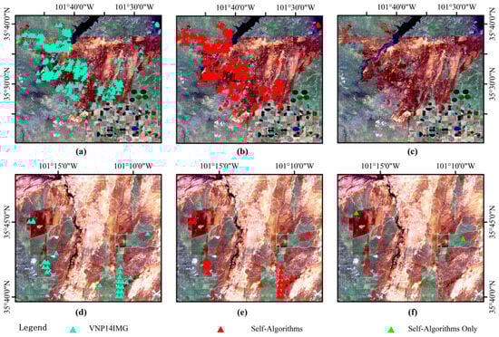
Figure 14. Comparison of fire detection results for the Texas grassland fire in February 2024. (a,d) VNP14IMG detections; (b,e) detections from the proposed method; (c,f) pixels detected only by the proposed method. Panels (a–c) show Sub-region 1, and panels (d–f) show Sub-region 2. The high-resolution reference imagery was acquired on 10 March 2024.

3.3.2. Small-Scale Agricultural Residue Burning

Agricultural residue burning is often small, short-lived, and spatially fragmented, challenging the sensitivity of standard operational products (Figure 15). In this case study, the proposed method produces a denser and spatially plausible set of fire pixels and recovers baseline omissions within burned areas, improving completeness without introducing additional false alarms.

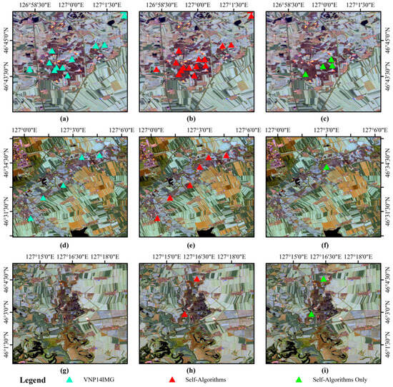
Figure 15. Comparison of crop residue burning detection results in Heilongjiang, China, from (25 October 2025 to 26 October 2025). The three rows correspond to three different local sub-regions. (a,d,g) VNP14 detections; (b,e,h) detections from the proposed method; (c,f,i) pixels detected only by the proposed method. The high-resolution reference imagery was acquired by Sentinel-2 on 26 October 2025.

3.4. Quantitative Accuracy Assessment

To quantify the trade-off between false-alarm suppression in high-interference zones and sensitivity to true fires, we construct a stratified validation dataset and report subset-specific metrics aligned with the purpose of each scenario.

3.4.1. Stratified Validation Dataset ($N=3435$)

Because active fires are sparse, random sampling often yields too few positive cases. We therefore adopt stratified sampling to build four scenario-oriented subsets (Table 6):

Table 6. Summary of the stratified validation dataset after excluding uncertain cases.

Subset	Purpose	N (Final)	True Fire	Non-Fire	Verification/Notes
Industrial/urban clusters	False-alarm suppression	986	0	986	High-res imagery + POI cross-check
Volcanic/geothermal regions	False-alarm suppression	178	0	178	High-res imagery + volcano/geothermal POI cross-check
Forest and grassland wildfires	Omission risk	1728	1728	0	Positive-only; uncertain cases excluded
Small-patch agricultural burning	Small-fire sensitivity	543	543	0	Positive-only; uncertain cases excluded
All (final)	-	3435	2271	1164	Initial candidates: 4000; excluded as uncertain: 565

Note: All counts are sample level, where one sample corresponds to one VIIRS 375 m candidate pixel. Non-fire-only subsets are used to quantify false alarms (FPR), while positive-only subsets are used to quantify omissions (OE/Recall).

(1)

Industrial/urban clusters (false-alarm suppression): heavy industrial zones (eastern China industrial belt, Middle East oil fields, Permian Basin), sampled within persistent-heat-source neighborhoods. $N=986$ (all non-fire).

(2)

Volcanic/geothermal regions (false-alarm suppression): crater-centered volcanic/geothermal hotspots sampled within persistent anomaly footprints. $N=178$ (all non-fire).

(3)

Forest and grassland wildfire regions (omission risk): representative wildfire events in 2024–2025 (e.g., Greece forest fires, Texas grassland fires), sampled within fire perimeters. $N=1728$ (all true fire).

(4)

Small-patch agricultural burning (small-fire sensitivity): agricultural regions in Northeast China and Southeast Asia. $N=543$ (all true fire).

Ground truth generation. Labels were generated in Google Earth Engine (GEE) using expert visual interpretation supported by spectral-index evidence. Cloud-free Sentinel-2 MSI and Landsat 8/9 OLI observations were matched within a ±1 day tolerance relative to the VIIRS overpass time (for nighttime overpasses, the nearest subsequent daytime acquisition within +1 day was used). Samples were labeled as true fire or non-fire based on visible smoke/flames/burn scars and NBR-based burn evidence. After excluding uncertain cases, the final dataset contains 2271 true fire samples and 1164 non-fire samples (true fire: non-fire ≈ 1.95:1).

PFM coverage proxy on labeled samples. To link the prior mask to labeled samples without re-running detection, we report the fraction of samples whose mapped 0.004° grid cell $\left(i_x,i_y\right)$ falls inside the post-processed PFM under each representative sensitivity setting (Table S2). We define wildfire coverage $C_{\mathrm{W}\mathrm{F}}=N_{\mathrm{W}\mathrm{F},\mathrm{m}\mathrm{a}\mathrm{s}\mathrm{k}}/N_{\mathrm{W}\mathrm{F}}$ and non-wildfire coverage $C_{\mathrm{N}\mathrm{W}}=N_{\mathrm{N}\mathrm{W},\mathrm{m}\mathrm{a}\mathrm{s}\mathrm{k}}/N_{\mathrm{N}\mathrm{W}}$, where $N_{\mathrm{W}\mathrm{F},\mathrm{m}\mathrm{a}\mathrm{s}\mathrm{k}}$ and $N_{\mathrm{N}\mathrm{W},\mathrm{m}\mathrm{a}\mathrm{s}\mathrm{k}}$ count samples inside the mask. These proxies indicate (i) the fraction of wildfire samples potentially affected by masked-regime switching and (ii) the extent to which the prior covers persistent non-wildfire false-alarm sources.

Definition and verification of non-wildfire false alarms. For industrial/urban and volcanic subsets, samples were selected from regions dominated by persistent non-wildfire anomalies. Non-fire labels were verified using high-resolution imagery and cross-checked with external POI datasets (power plants, gas flares, and Holocene volcanoes/geothermal areas). Since these subsets contain negatives only, any algorithm-reported “fire” is counted as a false alarm.

3.4.2. Quantitative Results and Analysis

All metrics are computed at the sample level using collocated high-resolution labels. We define TP (predicted fire and reference true fire), FP (predicted fire but reference non-fire), FN (predicted non-fire but reference true fire), and TN (predicted non-fire and reference non-fire). For subsets containing true fire positives, we report:

$$\mathrm{Commission}\mathrm{Error}(\mathrm{CE}):\mathrm{C}\mathrm{E}={\displaystyle \frac{FP}{TP+FP}}$$

(17)

$$\mathrm{Omission}\mathrm{Error}(\mathrm{OE}):\mathrm{O}\mathrm{E}={\displaystyle \frac{FN}{TP+FN}}$$

(18)

$$\mathrm{F}1\text{-}\mathrm{score}:F1={\displaystyle \frac{2TP}{2TP+FP+FN}}$$

(19)

For the industrial/urban and volcanic subsets (all negatives by construction; TP = 0), CE and F1 are not informative; we therefore report the false positive rate:

$$\mathrm{F}\mathrm{P}\mathrm{R}={\displaystyle \frac{FP}{N}},$$

(20)

where $N$ is the total number of samples in that subset (all negatives).

False-alarm suppression in high-interference zones (Table 7). In industrial/urban clusters, the operational product yields an FPR of 88.6% (874/986), whereas the proposed method reduces it to 22.7% (224/986). In volcanic regions, FPR decreases from 100.0% (178/178) to 57.3% (102/178), indicating effective suppression of static crater-centered interference while retaining sensitivity to strong signals that exceed adaptive thresholds.

Table 7. Quantitative comparison between the operational VNP14IMG and the proposed PFM/SHM-aware algorithm.

Region Type (Total)	Method	TP	FP	FN	CE	OE	F1-Score	FPR
Industrial/Urban (986)	VNP14	-	874	-	-	-	-	88.6%
	Ours	-	224	-	-	-	-	22.7%
Volcanic Regions (178)	VNP14	-	178	-	-	-	-	100.0%
	Ours	-	102	-	-	-	-	57.3%
Forest Fires (972)	VNP14	954	14	4	1.45%	0.42%	99.1%	-
	Ours	956	0	2	0.0%	0.21%	99.9%	-
Grassland Fires (756)	VNP14	749	4	2	0.53%	0.27%	99.6%	-
	Ours	751	1	0	0.13%	0.0%	99.9%	-
Crop Residue (543)	VNP14	482	0	61	0.0%	11.2%	94.0%	-
	Ours	536	0	7	0.0%	1.3%	99.3%	-

Note: For industrial/urban and volcanic subsets (where $TP=0$ by construction), we report FPR as the primary metric for suppression performance. For true fire subsets, CE/OE and F1 are reported.

True fire detection performance and small fire sensitivity. These reductions are not achieved at the expense of missed true fires: omission-related metrics remain low for forest and grassland fires (F1 > 99% for both methods). For small-patch agricultural burning, the proposed method substantially reduces omissions (OE: 11.2% → 1.3%) while maintaining zero commission error in this subset, improving F1 from 94.0% to 99.3%.

SHM-related failure mode. In our labeled wildfire subsets (forest/grassland and agriculture), SHM was not activated (activation rate = 0%), suggesting that SHM-triggered switching does not contribute to omissions in these cases. We note, however, that short-term stable anthropogenic burning could potentially trigger SHM under specific conditions, which warrants targeted future validation.

4. Discussion

The proposed PFM/SHM-aware framework is a lightweight spatiotemporal prior layer that can be overlaid on existing active fire detectors. It preserves upstream processing (radiometric calibration, geolocation, and brightness-temperature retrieval) and modifies only the pixel-level decision stage via prior-guided parameter switching. This modular design enables straightforward integration into operational pipelines, substantially reducing commission errors over industrial/urban environments with minimal implementation overhead and without altering the baseline system architecture. The resulting products are better suited for false-alarm-sensitive applications such as emergency response, emissions accounting, and industrial compliance monitoring.

The two priors play complementary operational roles. The PFM summarizes long-term recurring thermal patterns and is naturally updated on annual to multi-year cycles. The SHM, derived from multi-day nighttime stability statistics (e.g., a rolling $N_d$ day window), responds more quickly to newly commissioned or intensifying static sources and can be updated on weekly to monthly cycles depending on data availability. Together, they suppress recurrent non-wildfire anomalies while remaining responsive to short-term changes in industrial activity.

Parameter choices were guided by physical reasoning and quantitative trade-offs rather than ad hoc fitting. For PFM, the entropy threshold ($H_{norm}\ge 0.60$) filters strongly seasonal burning while retaining year-round sources. For SHM, the rolling window length targets a synoptic time scale to improve clear-sky observation probability, and the inclusion rule ($N_{hot}\ge 1$) is chosen to minimize cold-start latency. Masked-mode thresholds were calibrated using the systematic upper-tail shifts in anomaly indicators (Figure 7 and Figure 8) and a suppression–retention scan (Figure 9), ensuring robust rejection of persistent hotspots without overfitting.

Several limitations remain. (1) PFM quality depends on historical coverage; persistent clouds or data gaps can leave incomplete priors. (2) Building PFM from historical VNP14IMG introduces potential circularity; we mitigated this by using independent Sentinel-2/Landsat labels and POI cross-checks to confirm that the mask captures physical heat sources rather than product artifacts. (3) The SHM rule ($N_{hot}\ge 1)$ prioritizes timeliness but may occasionally over-flag under unstable backgrounds. (4) Strict masked thresholds could suppress true fires within complex industrial areas; operational safeguards (e.g., secondary screening or analyst review) can reduce this risk. (5) The ±1 day reference window may miss short-lived fires, so some valid detections may be mislabeled as false alarms, making reported precision conservative. Finally, although the underlying physical cues are broadly applicable, quantitative validation here emphasizes East Asia and selected global targets; performance in other biomes should be verified in future large-scale tests.

Future work will focus on (i) broader robustness calibration—systematic sensitivity analyses of key SHM parameters (e.g., $H_{min}$, $N_d$) across regions and seasons to quantify commission–omission trade-offs—and (ii) integration with learning-based detectors, using PFM/SHM as auxiliary inputs or weak supervision and combining them with complementary evidence (e.g., land-cover/industrial layers and cross-sensor consistency checks) to further reduce ambiguity under complex backgrounds.

5. Conclusions

This study proposes a PFM/SHM-aware contextual detection framework for a VIIRS 375 m contextual active fire detector by integrating PFM and SHM. By enabling prior-guided, pixel-level parameter switching within the contextual tests, the method targets static heat-source environments while keeping the overall algorithmic structure consistent with the baseline detector. Across our stratified evaluation dataset, the framework substantially reduces false alarms in high-interference zones (industrial/urban false positive rate from 88.6% to 22.7%; volcanic from 100.0% to 57.3%). At the same time, it maintains high sensitivity to biomass burning in the tested wildfire cases, with low omission errors for forest and grassland fires (forest: 0.42% to 0.21%; grassland: 0.27% to 0.0%). For low-intensity, fragmented agricultural burning, omission error decreases from 11.2% to 1.3% and the F1-score increases from 94.0% to 99.3%.

Overall, these findings indicate that combining long- and short-term spatiotemporal priors can improve the robustness and interpretability of contextual VIIRS fire detection in the evaluated scenarios, particularly where persistent non-wildfire heat sources dominate commission errors. The approach relies on historical recurrence statistics and nighttime stability patterns; therefore, broader cross-region and cross-season testing, along with assessments of prior update strategies and sensitivity to observation conditions, will be important for characterizing generalization and supporting practical deployment.

References

- Jones, M.W.; Santín, C.; Van Der Werf, G.R.; Doerr, S.H. Global Fire Emissions Buffered by the Production of Pyrogenic Carbon. Nat. Geosci. 2019, 12, 742–747. [Google Scholar] [CrossRef]
- van der Werf, G.R.; Randerson, J.T.; Giglio, L.; van Leeuwen, T.T.; Chen, Y.; Rogers, B.M.; Mu, M.; van Marle, M.J.E.; Morton, D.C.; Collatz, G.J.; et al. Global Fire Emissions Estimates during 1997–2016. Earth Syst. Sci. Data 2017, 9, 697–720. [Google Scholar] [CrossRef]
- Gajendiran, K.; Kandasamy, S.; Narayanan, M. Influences of Wildfire on the Forest Ecosystem and Climate Change: A Comprehensive Study. Environ. Res. 2024, 240, 117537. [Google Scholar] [CrossRef] [PubMed]
- Xu, W.; Wooster, M.J. Sentinel-3 SLSTR Active Fire (AF) Detection and FRP Daytime Product—Algorithm Description and Global Intercomparison to MODIS, VIIRS and Landsat AF Data. Sci. Remote Sens. 2023, 7, 100087. [Google Scholar] [CrossRef]
- Schroeder, W.; Oliva, P.; Giglio, L.; Csiszar, I.A. The New VIIRS 375 m Active Fire Detection Data Product: Algorithm Description and Initial Assessment. Remote Sens. Environ. 2014, 143, 85–96. [Google Scholar] [CrossRef]
- Di Biase, V.; Laneve, G. Geostationary Sensor Based Forest Fire Detection and Monitoring: An Improved Version of the SFIDE Algorithm. Remote Sens. 2018, 10, 741. [Google Scholar] [CrossRef]
- Zhang, N.; Sun, L.; Sun, Z.; Qu, Y. Detecting Low-Intensity Fires in East Asia Using VIIRS Data: An Improved Contextual Algorithm. Remote Sens. 2021, 13, 4226. [Google Scholar] [CrossRef]
- Chen, J.; Zheng, W.; Wu, S.; Liu, C.; Yan, H. Fire Monitoring Algorithm and Its Application on the Geo-Kompsat-2A Geostationary Meteorological Satellite. Remote Sens. 2022, 14, 2655. [Google Scholar] [CrossRef]
- Giglio, L.; Schroeder, W.; Justice, C.O. The Collection 6 MODIS Active Fire Detection Algorithm and Fire Products. Remote Sens. Environ. 2016, 178, 31–41. [Google Scholar] [CrossRef]
- Zhang, N.; Sun, L.; Sun, Z. GF-4 Satellite Fire Detection with an Improved Contextual Algorithm. IEEE J. Sel. Top. Appl. Earth Obs. Remote Sens. 2022, 15, 163–172. [Google Scholar] [CrossRef]
- Maeda, N.; Tonooka, H. Early Stage Forest Fire Detection from Himawari-8 AHI Images Using a Modified MOD14 Algorithm Combined with Machine Learning. Sensors 2023, 23, 210. [Google Scholar] [CrossRef]
- Dong, Z.; Yu, J.; An, S.; Zhang, J.; Li, J.; Xu, D. Forest Fire Detection of FY-3D Using Genetic Algorithm and Brightness Temperature Change. Forests 2022, 13, 963. [Google Scholar] [CrossRef]
- Li, Y.; Vodacek, A.; Kremens, R.L.; Ononye, A.; Tang, C. A Hybrid Contextual Approach to Wildland Fire Detection Using Multispectral Imagery. IEEE Trans. Geosci. Remote Sens. 2005, 43, 2115–2126. [Google Scholar] [CrossRef]
- Hally, B.; Wallace, L.; Reinke, K.; Jones, S.; Skidmore, A. Advances in Active Fire Detection Using a Multi-Temporal Method for next-Generation Geostationary Satellite Data. Int. J. Digit. Earth 2019, 12, 1030–1045. [Google Scholar] [CrossRef]
- Freeborn, P.H.; Wooster, M.J.; Roberts, G.; Xu, W. Evaluating the SEVIRI Fire Thermal Anomaly Detection Algorithm across the Central African Republic Using the MODIS Active Fire Product. Remote Sens. 2014, 6, 1890–1917. [Google Scholar] [CrossRef]
- Wooster, M.J.; Roberts, G.J.; Giglio, L.; Roy, D.P.; Freeborn, P.H.; Boschetti, L.; Justice, C.; Ichoku, C.; Schroeder, W.; Davies, D.; et al. Satellite Remote Sensing of Active Fires: History and Current Status, Applications and Future Requirements. Remote Sens. Environ. 2021, 267, 112694. [Google Scholar] [CrossRef]
- Mota, B.W.; Pereira, J.M.C.; Oom, D.; Vasconcelos, M.J.P.; Schultz, M. Screening the ESA ATSR-2 World Fire Atlas (1997–2002). Atmos. Chem. Phys. 2006, 6, 1409–1424. [Google Scholar] [CrossRef]
- Hall, J.V.; Zhang, R.; Schroeder, W.; Huang, C.; Giglio, L. Validation of GOES-16 ABI and MSG SEVIRI Active Fire Products. Int. J. Appl. Earth Obs. Geoinf. 2019, 83, 101928. [Google Scholar] [CrossRef]
- Jang, E.; Kang, Y.; Im, J.; Lee, D.-W.; Yoon, J.; Kim, S.-K. Detection and Monitoring of Forest Fires Using Himawari-8 Geostationary Satellite Data in South Korea. Remote Sens. 2019, 11, 271. [Google Scholar] [CrossRef]
- Ding, Y.; Wang, M.; Fu, Y.; Zhang, L.; Wang, X. A Wildfire Detection Algorithm Based on the Dynamic Brightness Temperature Threshold. Forests 2023, 14, 477. [Google Scholar] [CrossRef]
- Giglio, L.; Descloitres, J.; Justice, C.O.; Kaufman, Y.J. An Enhanced Contextual Fire Detection Algorithm for MODIS. Remote Sens. Environ. 2003, 87, 273–282. [Google Scholar] [CrossRef]
- Justice, C.O.; Giglio, L.; Korontzi, S.; Owens, J.; Morisette, J.T.; Roy, D.; Descloitres, J.; Alleaume, S.; Petitcolin, F.; Kaufman, Y. The MODIS Fire Products. Remote Sens. Environ. 2002, 83, 244–262. [Google Scholar] [CrossRef]
- Liu, C.; Chen, R.; He, B. Integrating Machine Learning and a Spatial Contextual Algorithm to Detect Wildfire from Himawari-8 Data in Southwest China. Forests 2023, 14, 919. [Google Scholar] [CrossRef]
- Zhang, D.; Huang, C.; Gu, J.; Hou, J.; Zhang, Y.; Han, W.; Dou, P.; Feng, Y. Real-Time Wildfire Detection Algorithm Based on VIIRS Fire Product and Himawari-8 Data. Remote Sens. 2023, 15, 1541. [Google Scholar] [CrossRef]
- Jin, S.; Wang, T.; Huang, H.; Zheng, X.; Li, T.; Guo, Z. A Self-Adaptive Wildfire Detection Algorithm by Fusing Physical and Deep Learning Schemes. Int. J. Appl. Earth Obs. Geoinf. 2024, 127, 103671. [Google Scholar] [CrossRef]
- El-Madafri, I.; Peña, M.; Olmedo-Torre, N. The Wildfire Dataset: Enhancing Deep Learning-Based Forest Fire Detection with a Diverse Evolving Open-Source Dataset Focused on Data Representativeness and a Novel Multi-Task Learning Approach. Forests 2023, 14, 1697. [Google Scholar] [CrossRef]
- Johnston, J.M.; Johnston, L.M.; Wooster, M.J.; Brookes, A.; McFayden, C.; Cantin, A.S. Satellite Detection Limitations of Sub-Canopy Smouldering Wildfires in the North American Boreal Forest. Fire 2018, 1, 28. [Google Scholar] [CrossRef]
- Zhang, T.; Wooster, M.J.; Xu, W. Approaches for Synergistically Exploiting VIIRS I- and M-Band Data in Regional Active Fire Detection and FRP Assessment: A Demonstration with Respect to Agricultural Residue Burning in Eastern China. Remote Sens. Environ. 2017, 198, 407–424. [Google Scholar] [CrossRef]
- Son, M.-W.; Kim, C.-G.; Kim, B.-S. Development of an Algorithm for Assessing the Scope of Large Forest Fire Using VIIRS-Based Data and Machine Learning. Remote Sens. 2024, 16, 2667. [Google Scholar] [CrossRef]
- Caseiro, A.; Rücker, G.; Tiemann, J.; Leimbach, D.; Lorenz, E.; Frauenberger, O.; Kaiser, J.W. Persistent Hot Spot Detection and Characterisation Using SLSTR. Remote Sens. 2018, 10, 1118. [Google Scholar] [CrossRef]
- Liu, Y.; Hu, C.; Zhan, W.; Sun, C.; Murch, B.; Ma, L. Identifying Industrial Heat Sources Using Time-Series of the VIIRS Nightfire Product with an Object-Oriented Approach. Remote Sens. Environ. 2018, 204, 347–365. [Google Scholar] [CrossRef]
- Ma, C.; Yang, J.; Chen, F.; Ma, Y.; Liu, J.; Li, X.; Duan, J.; Guo, R. Assessing Heavy Industrial Heat Source Distribution in China Using Real-Time VIIRS Active Fire/Hotspot Data. Sustainability 2018, 10, 4419. [Google Scholar] [CrossRef]
- Elvidge, C.D.; Zhizhin, M.; Hsu, F.-C.; Baugh, K.E. VIIRS Nightfire: Satellite Pyrometry at Night. Remote Sens. 2013, 5, 4423–4449. [Google Scholar] [CrossRef]
- Ma, C.; Li, T.; Sui, X.; Liao, R.; Xie, Y.; Zhang, P.; Wu, M.; Wang, D. Annual Dynamics of Global Remote Industrial Heat Sources Dataset from 2012 to 2021. Sci. Data 2024, 11, 631. [Google Scholar] [CrossRef]
- Elvidge, C.D.; Zhizhin, M.; Sparks, T.; Ghosh, T.; Pon, S.; Bazilian, M.; Sutton, P.C.; Miller, S.D. Global Satellite Monitoring of Exothermic Industrial Activity via Infrared Emissions. Remote Sens. 2023, 15, 4760. [Google Scholar] [CrossRef]
- Hong, Z.; Tang, Z.; Pan, H.; Zhang, Y.; Zheng, Z.; Zhou, R.; Ma, Z.; Zhang, Y.; Han, Y.; Wang, J.; et al. Active Fire Detection Using a Novel Convolutional Neural Network Based on Himawari-8 Satellite Images. Front. Environ. Sci. 2022, 10, 794028. [Google Scholar] [CrossRef]
- Hu, X.; Ban, Y.; Nascetti, A. Sentinel-2 MSI Data for Active Fire Detection in Major Fire-Prone Biomes: A Multi-Criteria Approach. Int. J. Appl. Earth Obs. Geoinf. 2021, 101, 102347. [Google Scholar] [CrossRef]
- Schroeder, W.; Oliva, P.; Giglio, L.; Quayle, B.; Lorenz, E.; Morelli, F. Active Fire Detection Using Landsat-8/OLI Data. Remote Sens. Environ. 2016, 185, 210–220. [Google Scholar] [CrossRef]
- Byers, L.; Friedrich, J.; Hennig, R.; Kressig, A.; Li, X.; Valeri, L.M.; McCormick, C. A Global Database of Power Plants. 2018. Available online: https://www.wri.org/research/global-database-power-plants (accessed on 29 December 2025).
- Elvidge, C.D.; Zhizhin, M.; Baugh, K.; Hsu, F.-C.; Ghosh, T. Methods for Global Survey of Natural Gas Flaring from Visible Infrared Imaging Radiometer Suite Data. Energies 2016, 9, 14. [Google Scholar] [CrossRef]
Disclaimer/Publisher’s Note: The statements, opinions and data contained in all publications are solely those of the individual author(s) and contributor(s) and not of MDPI and/or the editor(s). MDPI and/or the editor(s) disclaim responsibility for any injury to people or property resulting from any ideas, methods, instructions or products referred to in the content. |
© 2026 by the authors. Licensee MDPI, Basel, Switzerland. This article is an open access article distributed under the terms and conditions of the Creative Commons Attribution (CC BY) license.