Article

Constraining the Trajectory of Glacier Loss in the Cordillera Real (Bolivia) via a Time-Evolving Inventory


by
Giuliana Adrianzen
and
Andrew G. O. Malone
*
Department of Earth and Environmental Sciences, University of Illinois Chicago, Chicago, IL 60607, USA
*
Author to whom correspondence should be addressed.
Remote Sens. 2026, 18(6), 905; https://doi.org/10.3390/rs18060905
Submission received: 31 December 2025 / Revised: 7 March 2026 / Accepted: 10 March 2026 / Published: 16 March 2026
(This article belongs to the Special Issue Remote Sensing of the Cryosphere (Third Edition))

Highlights

What are the main findings?
  • Glaciers in the Cordillera Real lost 103.67 ± 9.97 km2 (42.0 ± 2.1%) of glacierized area between 1992 and 2024.
  • The loss rate has been relatively constant over this 32-year interval at an absolute rate of 2.99 [2.32, 3.67] km2 yr−1 and a fractional loss rate of 1.6 [1.3, 1.9]% yr−1, resolving disagreement among past studies on the trajectory of glacier loss.
What are the implications of the main finding?
  • Deglaciation could occur by the early 2070s, or only about a fifth (22%) of the glacierized area could remain by the end of the century (2100 CE), based on two models for the trajectory of glacier loss.
  • Much of the remaining ice is at risk, especially under unabated climate change (SSP5-8.5); even for a moderate climate future (SSP2-4.5), less than half of the current glacierized area would be above the predicted end-of-century equilibrium line altitude.

Abstract

Bolivia is home to approximately 20% of the tropical glaciers in South America, which are sensitive indicators of climate change and critical water resources. Glaciers in the Cordillera Real supply meltwater to Bolivia’s administrative capital, La Paz, making it important to accurately assess their evolution. This study reassesses the trajectory of glacier loss in the Cordillera Real between 1992 and 2024. We construct a time-evolving glacier inventory utilizing remote sensing data (Landsat) and techniques to limit the impact of ephemeral snow cover. Our inventory is at a temporal resolution (5- to 8-year spacing) that allows us to assess the trajectory of glacier loss using statistical models. Between 1992 and 2024, the Cordillera Real lost 103.67 ± 9.97 km2 of glacierized area, representing a 42.0 ± 2.1% reduction. We find that glaciers in the Cordillera Real have been retreating at a constant absolute loss rate of 2.99 [2.32, 3.67] km2 yr−1 and a constant fractional loss rate of 1.6 [1.3, 1.9]% yr−1, contrasting with past studies that suggest accelerating or decelerating loss rates. Our findings provide new insights into the current extent of glaciers in the Cordillera Real and their longevity. The time-evolving inventory is available for use in future studies on the evolution of glaciers in the Cordillera Real and the impacts of their continued loss.

1. Introduction

Tropical glaciers are found in high-altitude mountain ranges such as the Andes of South America, which are home to 99% of tropical glaciers [1]. These glaciers are highly sensitive indicators of climate change as they react quickly to climatic variations [2,3]. The retreat of tropical glaciers is thought to have accelerated since the 1980s [1,4,5,6,7,8,9,10]. Many small (<0.5 km2) tropical glaciers, especially those at lower elevations, are expected to disappear in the coming few decades [3,9,11].
The retreat and disappearance of tropical glaciers pose societal challenges to downstream communities. Tropical glaciers are important to local communities that rely on glacial meltwater for agriculture, domestic consumption, and hydropower, and they also hold cultural significance [12]. The runoff of glaciers in the outer tropics (Bolivia and Peru) also helps maintain streamflow during the dry season, which spans from May to September [3,13]. With the retreat of glaciers also comes the formation and expansion of potentially hazardous glacial lakes, which pose a threat from the risk of glacial lake outburst floods [14,15,16]. Tracking glacial changes is thus crucial for informing local communities of glacierized area changes so that they may be prepared for decreasing access to water resources in the Andes in the event of continued glacier loss and disappearance.
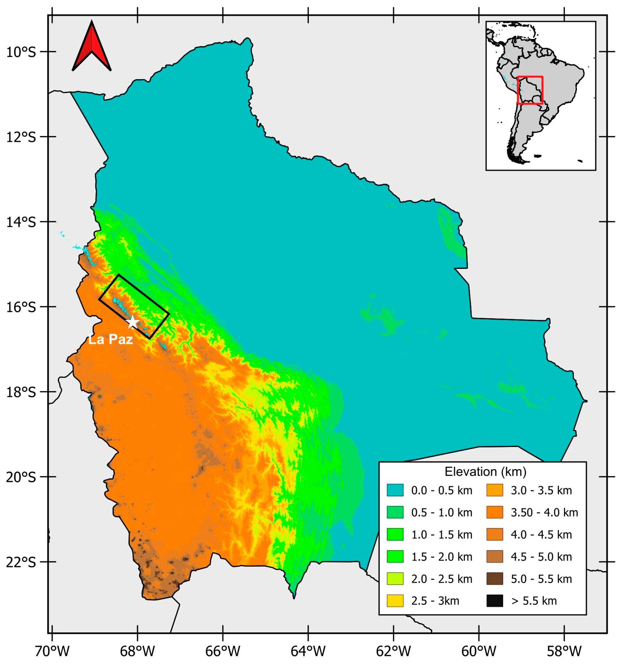
Bolivia is home to 20% of the remaining tropical glaciers [1] found within the high peaks of the Andes (Figure 1). More than half of the Bolivian glaciers are located in the Cordillera Real, which accounts for 11% of total tropical glaciers globally [17]. Runoff from glaciers in the Cordillera Real provides water resources for nearby communities, including the regional administrative capital, La Paz, and neighboring El Alto [12,18]. Glacial meltwater helps maintain consistent water flow during the dry season, which lasts from May through September, when there is decreased precipitation [19,20,21]. During the dry season, glacial melt contributes to 27% of water resources for La Paz [18], making glaciers in the Cordillera Real a crucial water resource that is retreating rapidly.
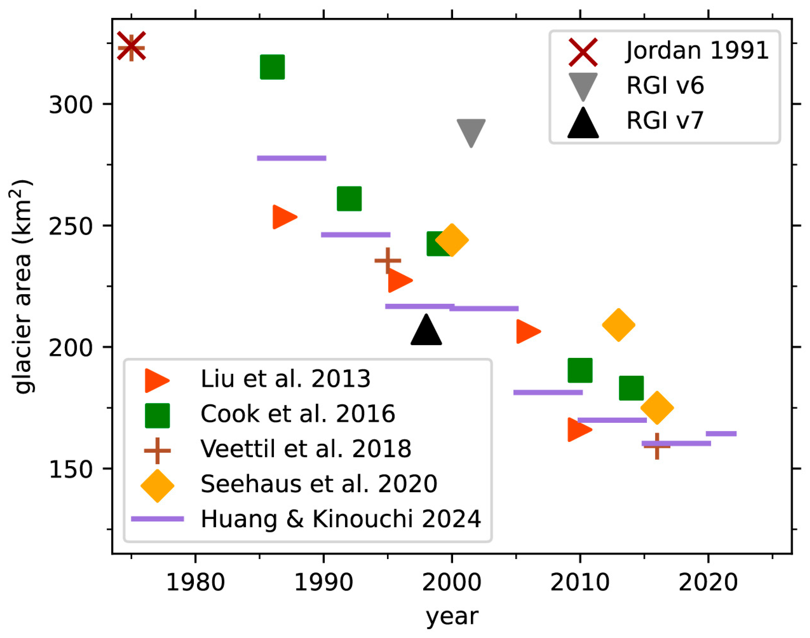
Past studies have inventoried and quantified glacier change in the Cordillera Real, noting rapid glacier-area decline in recent decades [14,16,17,24,25]. However, there is disagreement on the trajectory of glacier loss (Figure 2). Some studies report recent acceleration in the loss rate [17,24,25], whereas others find a deceleration in the loss rate [14,16]. One study even reported little to no change in glacier area from the mid-2010s through the early 2020s [16]. Some studies have also identified alternating patterns of higher and lower loss rates [16,24]. Disagreement in the trajectory of glacier loss complicates efforts to assess their future role as a water resource.
This disagreement among past studies may stem from how the glacier areas were quantified. Monitoring glaciers across the Cordillera Real requires remote sensing data and techniques, which can be impacted by scene selection. Most previous studies have analyzed scenes from the dry season (May to September) under the assumption that reduced precipitation minimizes misclassification of ephemeral snow cover as glacier extent [14,17]. However, two studies from the outer tropics of Peru show that dry-season scenes can overestimate glacier areas relative to scenes from October through December (i.e., after the nominal dry period) [28,29]. Glacier area estimates can also be affected by the phase of the El Niño–Southern Oscillation (ENSO) [29]. During El Niño events (positive phase), the outer tropics tend to be warmer and drier [3,11], with elevated glacier melting [8], thereby reducing the likelihood of overestimating the glacierized area due to ephemeral snow cover. Thus, past studies may have overestimated glacier areas in some years due to the season and the ENSO phase of their remote sensing data.
Disagreement on the trajectory of glacier loss may also arise from how changes in the loss rate were identified. Most past studies in the Cordillera Real quantified loss rates by differencing glacier area between two observation years [16,17,24,25]. If the calculated rate differs between early and later intervals, the loss rate is inferred to have changed. However, this approach is highly sensitive to errors in the glacier area estimates, particularly those related to ephemeral snow cover. One study instead estimated the loss rates via a statistical model, finding that their glacier area estimates follow an exponential decay trajectory (i.e., constant fractional loss rate) [14]. Two studies using a similar statistical approach for glacierized areas in the outer tropics of Peru found that the long-term trajectory follows a linear model (i.e., constant loss rate), with individual measurements varying from the trend due to ephemeral snow cover [28,29]. Many past studies for the Cordillera Real, however, have too few measurements to evaluate statistical models for glacier loss.
This study reassesses the trajectory of glacier loss in the Cordillera Real by constructing a time-evolving glacier inventory from 1992 to 2024. Our inventory utilizes methods not previously implemented in the Cordillera Real to reduce the influence of ephemeral snow cover on our glacier mapping. These include restricting data collection to years with at least moderate El Niño events, using the composite method of Taylor et al. (2022) [30], and, when possible, including a scene in the composites from after the nominal dry period as recommended by Kochtitzky et al. (2018) [28] and Malone et al. (2022) [29]. Since our inventory contains six estimates of glacier area, we can evaluate the trajectory of glacier loss using statistical models rather than via the two-point differencing approach. We test three trajectories of glacier loss, which are consistent with findings from previous studies: (1) linear model (i.e., constant loss rate), (2) quadratic model (i.e., accelerating/decelerating loss rate), and (3) exponential decay model (i.e., constant fractional loss rate). This study provides new insights into the amount of glacier area and the trajectory of glacier loss in the Cordillera Real. Shapefiles of the glacier extents in our time-evolving inventory are available in the Supplementary Materials.

2. Materials and Methods

2.1. Datasets

2.1.1. Landsat Scenes

We utilized top-of-atmosphere reflectance Landsat scenes (Collection 2, Level 1) to assess glacier change in the Cordillera Real. Top-of-atmosphere Landsat scenes were used in the Taylor et al. (2022) [30] study that introduced the annual composite method implemented in this study, as well as in a recent study of glaciers in the Cordillera Real [16]. The six years selected for analysis were associated with El Niño conditions: 1992, 1998, 2005, 2010, 2016, and 2024. El Niño conditions in the outer tropics are warmer and drier [3,11], making these years good for monitoring glaciers due to reduced snow and cloud cover. The selected years span a range of El Niño intensities from weak (2005) to very strong (1998, 2016) (https://ggweather.com/enso/oni.htm (accessed 1 June 2025)).
For each year, we generated a composite image using multiple Landsat scenes, following the methodology from Taylor et al. (2022) [30]. Composite images were constructed in Google Earth Engine (accessed 15 May 2025) and served as inputs for the glacier mapping algorithm (Section 2.2). At least three scenes with minimal cloud cover over the glacierized area and little visible snow cover were selected annually (Table 1), and the median pixel values were used in the composite. This approach can reduce cloud and snow contamination compared to single-scene analyses [30].
Scenes were selected based on minimal snow and cloud cover, with a preference for imagery acquired during the dry season, which typically spans May to September in the outer tropics [3]. The reduction in precipitation during this period generally results in decreased cloud formation and limited snow accumulation. Precipitation patterns are further influenced by ENSO phases: El Niño events reduce precipitation by approximately 10–30%, often extending arid conditions into the austral summer months, whereas La Niña events, which are characterized by cooler and wetter conditions, tend to increase precipitation during this time [11]. In three of the six years analyzed (1992, 2010, 2024), at least one scene from October, November, or December (i.e., after the dry season) was also included. Scenes from this post-dry-season period have been shown to better capture extents of glaciers in the outer tropics of Peru, while those from the dry season may overestimate the glacierized area [28,29]. The other years (1998, 2005, 2016) did not have an optimal scene from this post-dry-season period, but they did have a scene from September.

2.1.2. Inventories

To validate our 1998 inventory and delineate boundaries of individual glaciers, we used version 7.0 of the Randolph Glacier Inventory (RGI v7.0) [22], which is a global inventory of glacier outlines. The RGI v7.0 glacier extents for the Cordillera Real are based on a 13 June 1998 Landsat scene, which is one of the scenes used in our inventory (Table 1). For glaciers in our inventory that are also in the RGI v7.0, we include their corresponding RGI identification number.
We also used glacier mass balance data from the World Glacier Monitoring Service (WGMS) [31] to approximate the regional equilibrium line altitude (ELA). The ELA of a glacier is roughly where on a glacier mass gain from accumulation equals mass loss from ablation, and it is a useful indicator for determining glacier health [32]. At Zongo Glacier in the Cordillera Real, previous studies report an average ELA of 5144 meters above sea level (m a.s.l.) for the period 1991–2006 [33], which has been used as an average regional ELA for the Cordillera Real [16,25]. To determine an updated regional ELA, we retrieved the most recent ELA data for Zongo Glacier from the WGMS [31]. We calculated an average ELA of 5340 m a.s.l. for the most recent decade of available ELA values (2012–2021). This updated regional ELA is nearly 200 m higher than the earlier estimate, suggesting significant glacier disequilibrium over the past two decades.

2.1.3. Digital Elevation Model (DEM)

As part of the glacier-mapping algorithm and to characterize the topography of glaciers in the Cordillera Real, we used the Shuttle Radar Topography Mission (SRTM) Version 3 SRTM GL1 digital elevation model (DEM), obtained via www.opentopography.org (accessed on 14 May 2025) [23]. The SRTM GL1 DEM offers a spatial resolution of 30 m, consistent with the Landsat imagery used in this study. To ensure spatial congruence, the DEM was resampled to the Landsat grid using nearest-neighbor interpolation. The DEM was integrated into the processing workflow to facilitate the removal of proglacial lakes (Section 2.2) and to derive topographic metrics for each glacier in the inventory (Section 2.3).

2.2. Glacier Mapping

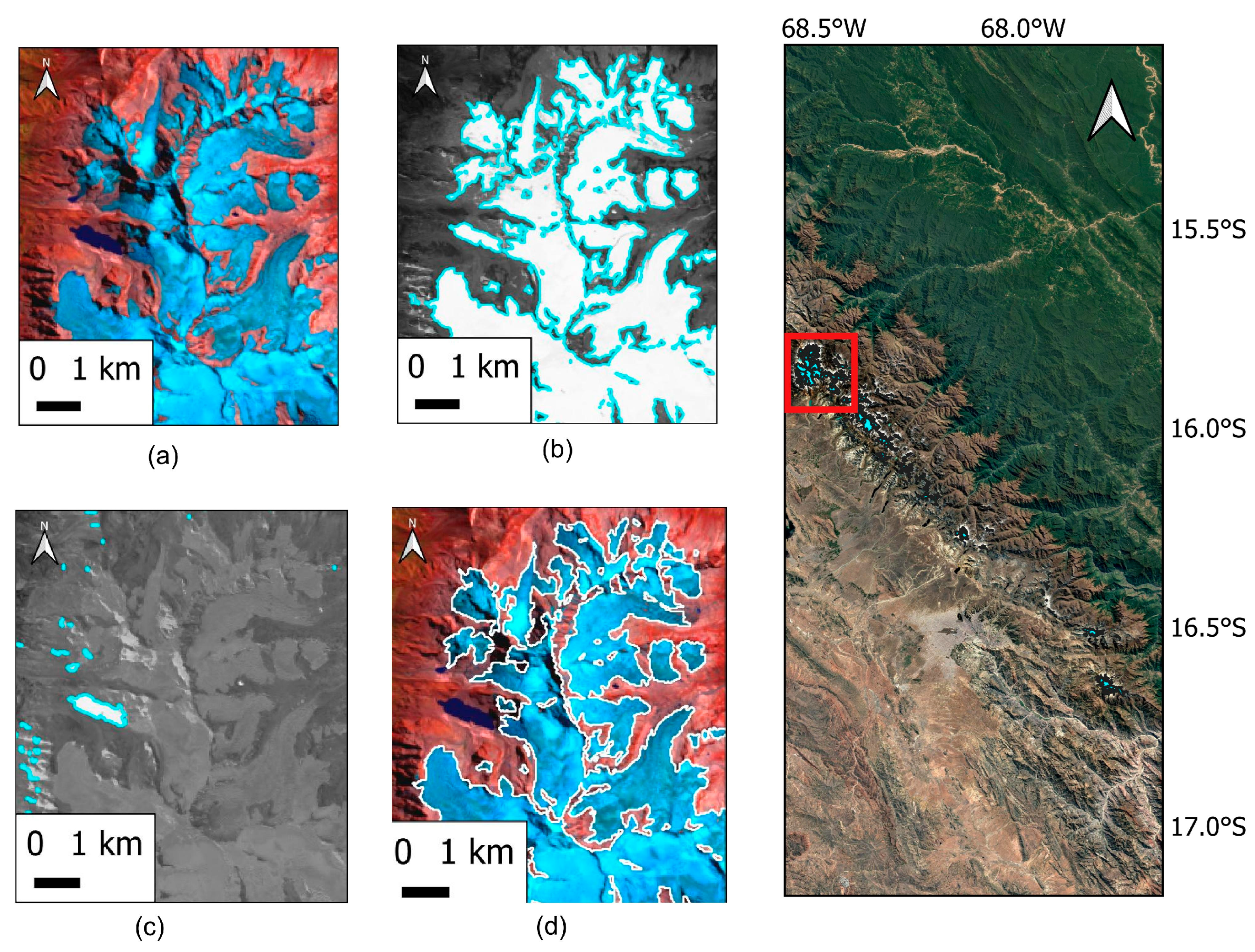
Glacier mapping was performed in QGIS (version 3.40), applying a semi-automated delineation algorithm (Figure 3). Since glaciers in Bolivia are mainly clean-ice glaciers [14], optical remote sensing techniques such as band ratios [14,24], the normalized difference snow index (NDSI) [16,17], or a combination of both methods [25] have been used to inventory glaciers. To classify snow and ice, we used the NDSI [34]:
NDSI = (Green Band − SWIR1 Band)/(Green Band + SWIR1 Band).
Following a comprehensive analysis of NDSI histograms, a threshold value of 0.5 was selected to differentiate potential snow and ice pixels from non-glacierized areas (Figure 3b). This threshold is lower than those used in some past studies of glaciers in the outer tropics (e.g., [25,30]), suggesting we may find larger glacierized areas than in past studies. We performed a sensitivity analysis on our NDSI threshold and found that varying the threshold by ±0.05 resulted in changes in the total glacierized area that were smaller than the uncertainty in any year’s total glacierized area (Table A1).
The NDSI-based glacier mapping approach can misclassify proglacial lakes as part of the glacial extent (Figure 3b). To remove proglacial lakes classified as part of the glacierized area, we applied the lake identification method used by Hanshaw & Bookhagen (2014) [15] for mountainous terrain. We computed the Normalized Difference Water Index (NDWI) [35],
NDWI = (Blue Band − NIR Band)/(Blue Band + NIR Band)
to detect potential lakes. To exclude shadowed regions with large NDWI values, we incorporated a hillshade layer derived from the SRTM DEM. Pixels with NDWI values exceeding 0.2 and hillshade values above 50 (from a possible range of 0 to 255) were classified as potential lakes (Figure 3c) and were removed from the glacier masks. Finally, we edited the glacier masks, removing glacierized areas smaller than 6 pixels (0.0054 km2), filling holes in the glacierized area smaller than 9 pixels (0.0081 km2), and manually adjusting the glacier boundary when misplaced (Figure 3d). Manual edits altered the total glacierized area by less than half the uncertainty in the total glacierized area (Table A1). However, to accurately track the evolution of individual glacier basins, removing proglacial lakes and manual adjustments were necessary.
For each year of observation, we quantified the uncertainty associated with glacier area estimates using the method proposed by Hanshaw and Bookhagen (2014) [15], which has been adopted in subsequent studies (e.g., [14,16]). This approach assumes that the uncertainty in glacier area follows a Gaussian distribution and results from misclassification of pixels along the glacier’s boundary according to the following formula:
Uncertainty (1σ) = (P/G)·0.6827·G2/2,
where P is the glacier perimeter, G is the grid cell size (30 m for Landsat scenes), and the factor of 0.6827 represents the proportion of a Gaussian distribution found between ±1σ. We have corrected the value of this factor from Hanshaw and Bookhagen (2014) [15] where it was written as 0.6872, which we believe represents a transcription error. Uncertainties are presented as 2–σ uncertainty intervals (i.e., roughly the 95% confidence interval) and propagated in quadrature. Values are said to be significantly different if their 2–σ uncertainty intervals do not overlap, and differences in area are said to be significant if they exceed the 2–σ uncertainty interval.

2.3. Individual Glacier Analysis (Size, Basins, Thresholds)

We separated our glacier masks into individual glacier basins using the ice divides from the RGI v7.0. To quantify uncertainty for each glacier, we used Equation (3) but defined the perimeter as the length of the glacier’s boundary that does not abut another glacier. This definition of the perimeter ensures that the length where a glacier joins another glacier is not included in the uncertainty estimate, as outlined in Paul et al. (2017) [36]. We used the SRTM DEM to characterize the elevation, aspect, and slope of each glacier. To further track individual glacier changes, we categorized them by size: small (<0.5 km2), medium (≥0.5 km2 to <5.0 km2), and large (≥5.0 km2). A cutoff of <0.5 km2 has been used in previous studies to denote small glaciers [9,25]. Our cutoff between medium and large glaciers (5 km2) is smaller than the cutoff used by Seehaus et al. (2020) [25] (7.5 km2), since the largest glacier in the Cordillera Real within the RGI v7.0 is 6.77 km2. To ensure we categorized some glaciers as large, we used the threshold of 5 km2, which is an order of magnitude larger than our cutoff for small glaciers.

2.4. Statistical Analysis for Trends

To characterize the trajectory of glacier-area change in the Cordillera Real, we applied weighted least squares (WLS) regression to the glacier area time series from our inventory. We evaluated three candidate models: (1) linear, (2) quadratic, and (3) exponential decay (i.e., log-linear). The linear model represents a constant absolute loss rate (km2 yr−1), the quadratic model allows for acceleration or deceleration in the absolute loss rate (km2 yr−2), and the exponential decay model represents a constant fractional loss rate (proportional to the glacier area, % y−1). Measurement uncertainty was incorporated using inverse-variance weighting (1/σi2). For the linear and quadratic models, σi denotes the 1–σ uncertainty in glacier area for each year (Equation (3)). For the exponential model, regression was performed on log-transformed area values, with σi defined as the 1–σ relative uncertainty (σi/Ai). Regressions were implemented using the statsmodels (version 0.14.4) package in Python (version 3.12.2) [37].
We assessed model performance using the Akaike Information Criterion (AIC) [38]. Due to the small number of observations (n = 6), we utilized the small-sample corrected Akaike Information Criterion (AICc) [39,40,41]:
AICc = AIC + (2k(k + 1))/(n − k − 1),
where k is the number of estimated parameters (k = 2 for the linear and exponential decay models; k = 3 for the quadratic model) and n is the number of observations (n = 6). For the exponential decay model, the log-likelihood was calculated assuming log-normal errors, with the Jacobian term included to ensure that AIC values are directly comparable across models. We considered the model with the lowest AICc to be the best-supported model and used the differences in AICc (ΔAICc) to assess relative model support. Because of the limited sample size of our study (n = 6), higher-order models were not evaluated. Even the quadratic model only has three residual degrees of freedom, limiting its statistical power. As such, we could not statistically assess whether there were alternating periods of enhanced or reduced loss rates as suggested by some past studies [16,24].

3. Results

3.1. Inventory Assessment

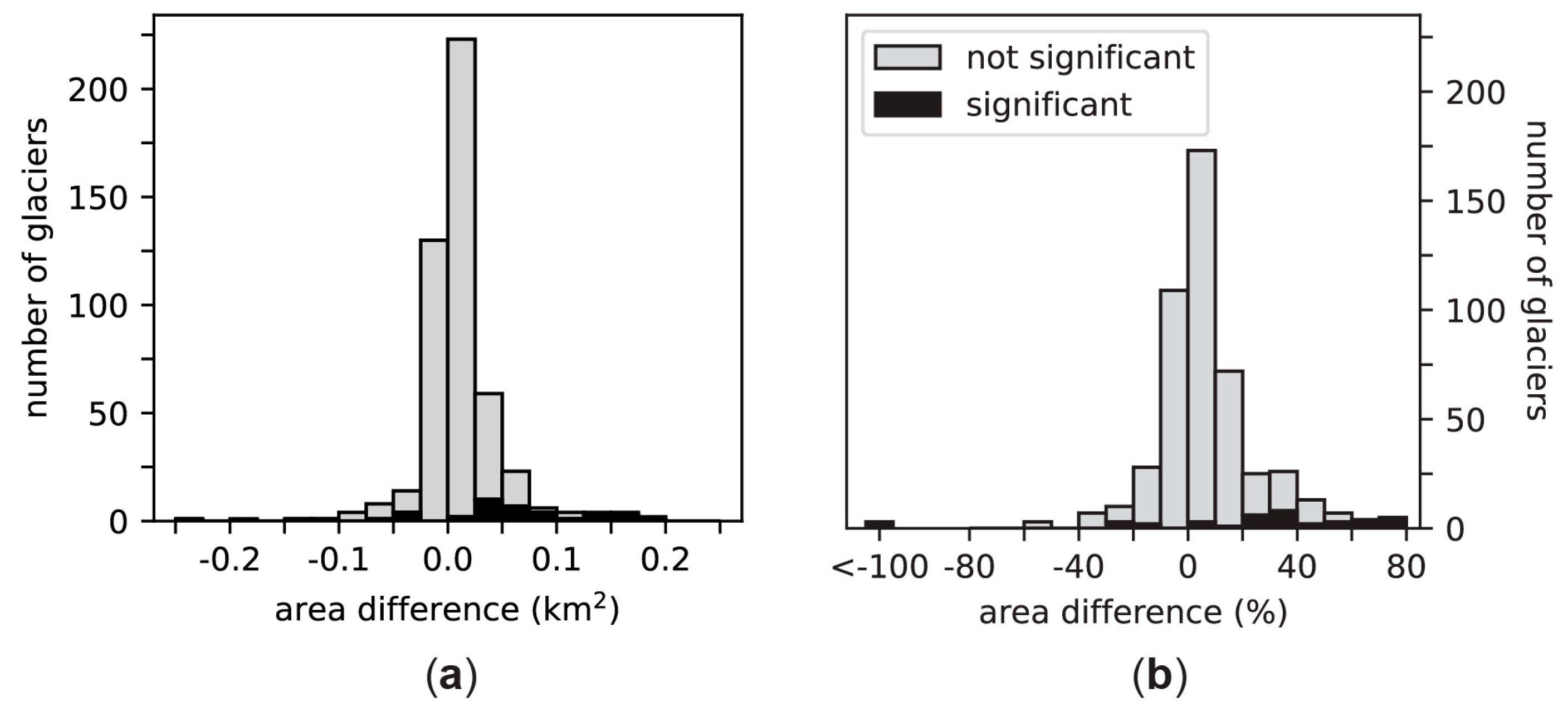
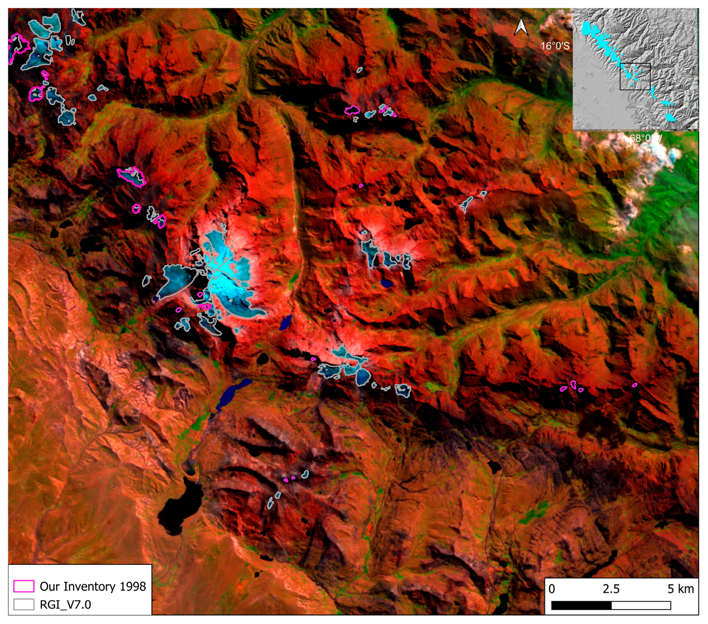
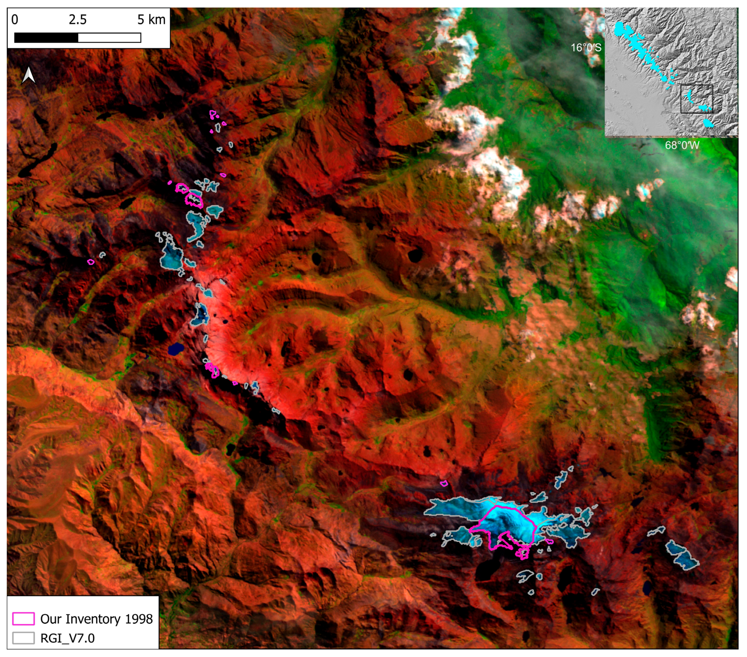
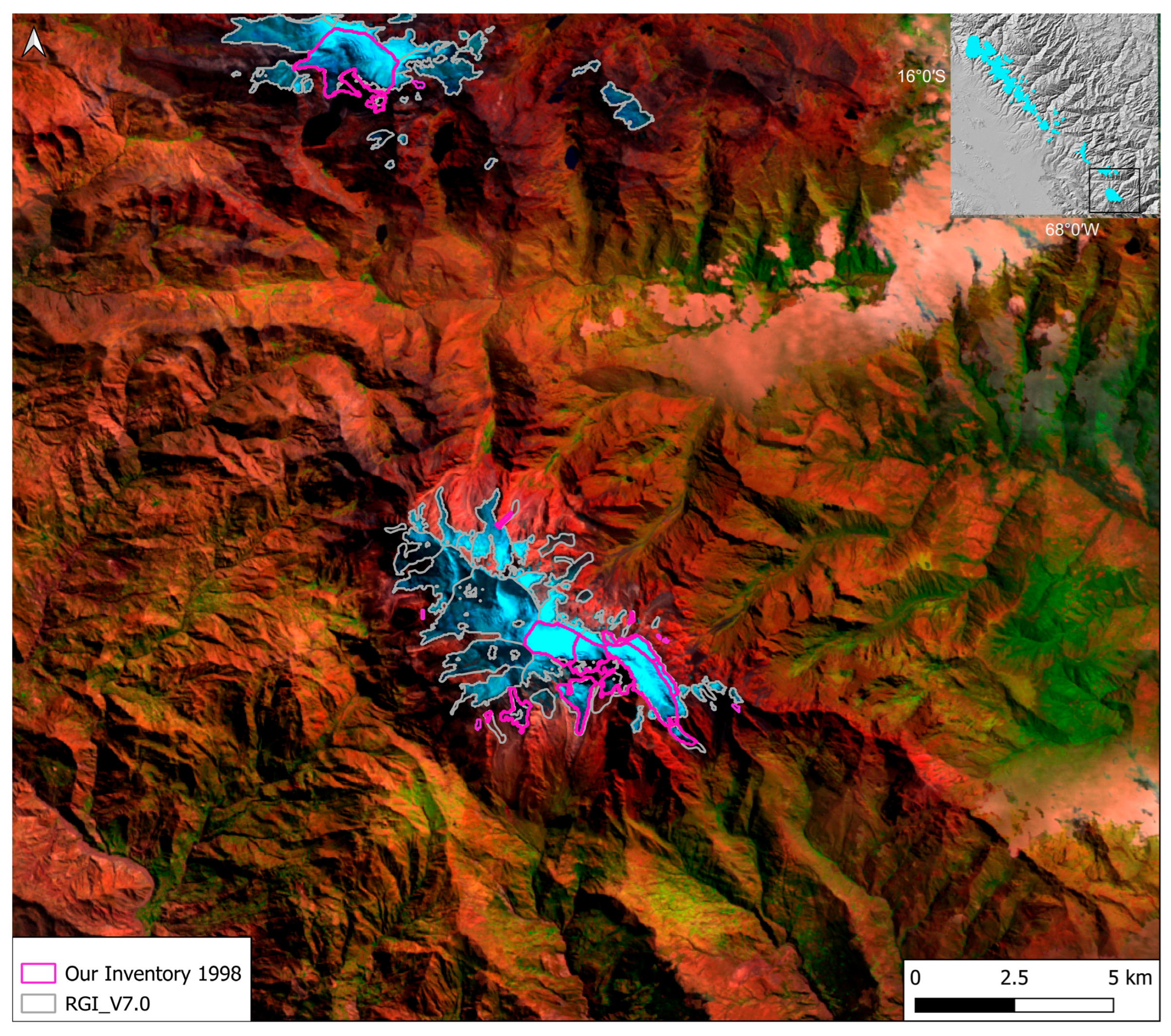
The glacierized area in our inventory in 1998 is statistically indistinguishable from that in the RGI v7.0, but it contains more glaciers (Table 2). The total glacierized area in the RGI v7.0 falls within the 2–σ uncertainty of our inventory’s total area (213.96 ± 7.93 km2). At the glacier-basin level, the two inventories have 485 basins in common, of which 446 glaciers (92.0%) have an RGI v7.0 glacier area that falls within the 2–σ uncertainty of our inventory (Figure A1). Our inventory, however, contains 83 additional glacier basins (Table 2). It identifies 82 glaciers not included within the RGI v.7.0. These glaciers not found in the RGI v7.0 have a total area of 1.57 km2 in 1998. The largest has an area of 0.1422 km2, and the smallest has an area of 0.0054 km2 (i.e., the threshold for the smallest glaciers in our inventory). In addition to having glaciers not found in the RGI v7.0, our inventory does not include two glaciers found in the RGI v.7.0 (RGI2000-v7.0-G-16-03094, RGI2000-v7.0-G-16-03498). These two glaciers fall within larger glacier basins, and thus their extents were included as part of the larger basins. A visual comparison of individual glacier basins between the two inventories is found in Appendix B (Figure A2, Figure A3, Figure A4, Figure A5, Figure A6 and Figure A7).
The distribution of glaciers in our inventory is comparable to the distribution in the RGI v7.0 (Table 2). Small glaciers (<0.5 km2) account for about 80% of the individual glaciers in our inventory and in the RGI v7.0 (81.9% and 80.1%) and contribute to almost a quarter of the total area (24.9%, 24.2%). Medium glaciers (≥0.5 km2 and <5.0 km2) contribute the most to the area in both inventories (60.84% and 61.1%) but account for less than a fifth of the glaciers (17.2%, 18.9%). The number and area of large glaciers (≥5.0 km2) are nearly identical in both inventories. Also, the direction the glaciers face (i.e., their aspect) is quite similar. About 60% of glaciers face southward (aspects of south, southeast, or southwest) in our inventory and in the RGI v7.0 (62.6% and 61.8%), and the distribution of area of southward-facing glaciers is nearly identical (61.5% and 61.8%). Our inventory has slightly more glaciers facing southward since nearly all (89.0%) of the glaciers in our inventory that are not found in the RGI v7.0 face southward. In total, our 1998 inventory is nearly indistinguishable from the RGI v7.0 in its total glacierized area and distribution of glaciers, but our inventory identifies glaciers not included in the RGI v7.0.

3.2. Glacier Changes, 1992 to 2024

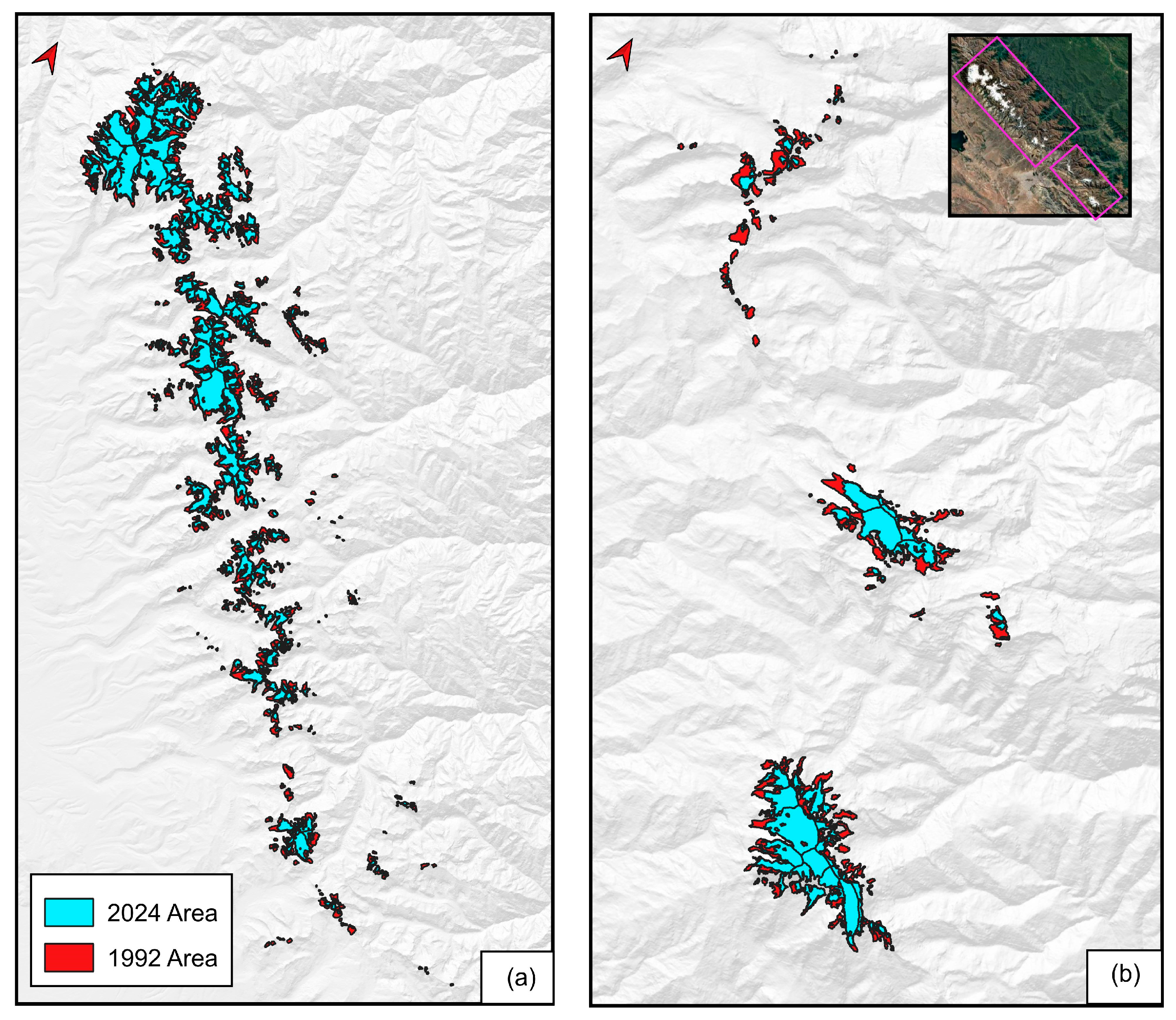
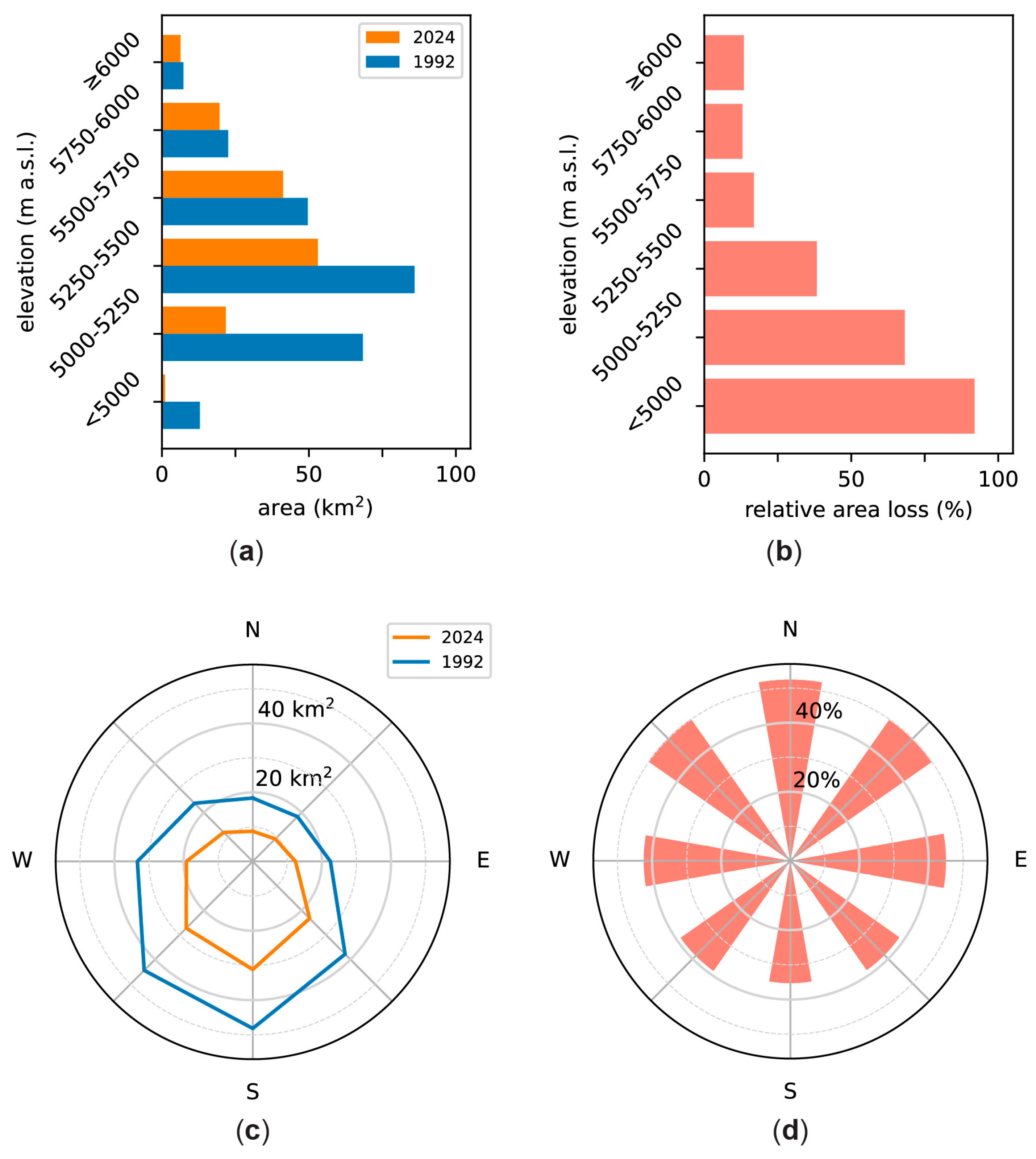
Between 1992 and 2024, glaciers in the Cordillera Real shrank (Figure 4). The glacierized area decreased from 246.67 ± 8.37 km2 to 143.00 ± 5.41 km2 (Table A2), representing a 42.0 ± 2.1% decrease in the glacierized area relative to 1992. Most (88.2%) of the area loss occurred below 5500 m.a.s.l. (Figure 5a). Below 5000 m a.s.l., nearly all (91.9%) of the glacierized area has vanished (Figure 5b). This disappearance, however, contributed only 11.5% to the total loss, reflecting the small amount of glacierized area in 1992 found at these lowest elevations. Loss of glacierized areas between 5000 and 5250 m a.s.l. contributed the most (45.0%) to the total loss, and 68.2% of the glacierized area in this range vanished. Above 5750 m a.s.l., 13.1% of the glacierized area has vanished, but this loss contributes less than 4% of the total area loss. Glacierized areas with a southward aspect (south, southwest, southeast) contributed the most to total area loss (Figure 5c), but this contribution may reflect the southward-facing orientation of glaciers in the Cordillera Real [17]. Glacierized areas with a northward aspect (north, northwest, northeast) have experienced a greater proportional loss (Figure 5d), which is consistent with higher mass-loss rates by norward-facing glaciers [25].
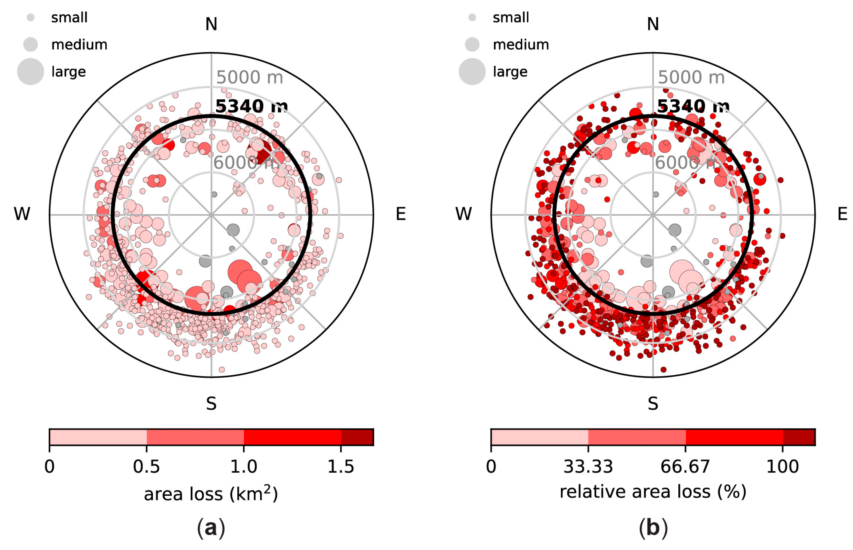
In addition to the loss in glacierized areas, the size and number of individual glaciers also decreased (Table A2 and Table A3). Between 1992 and 2024, the number of glaciers decreased from 655 to 509. Over that interval, 259 glaciers vanished, representing a loss of 39.5% of the glaciers in 1992. In addition, 88 glaciers broke apart into multiple glacierized areas, leading to a smaller reduction in the total number of glaciers than the number that vanished. The glacier with the largest absolute loss was a large, northeast-facing glacier, with a median elevation in 1992 of 5571 m a.s.l. (Figure 6a). The other individual glaciers with large area losses were large and medium glaciers, which have the most area to lose. The greatest contribution to area loss by size category was by glaciers characterized as medium in 1992. They accounted for 50.7% of the area loss, although their total area in 1992 contributed to 60.8% of the total glacierized area. Small glaciers also contributed notably to glacier loss, accounting for 43.9% of the area loss while only contributing 24.9% to the glacierized area in 1992.
While medium glaciers contributed the most to total area loss, and some large glaciers accounted for the greatest area loss by individual glaciers, small glaciers experienced the most dire relative losses (Figure 6b). Glaciers considered small in 1992 were the only ones to completely vanish (relative loss = 100%), and 92.7% of small glaciers lost at least half of their area between 1992 and 2024. Only 25.6% of medium glaciers lost at least half of their area over that period, and no large glaciers lost more than 25.8% of their area. Glaciers at lower elevations were also particularly vulnerable to loss. Nearly all (96.2%) small glaciers in 1992 with a median elevation below the recent average ELA at Zongo glacier (5340 m a.s.l.) lost at least half of their area. For medium glaciers with a median elevation below 5340 m a.s.l., 41.1% lost at least half of their area. No large glaciers had a median elevation below 5400 m a.s.l. (i.e., the threshold for highly vulnerable glaciers in the outer tropics [13]). Glaciers with median elevations at higher elevations tended to be more resilient, but with some differences based on aspect. Northward-facing glaciers experienced higher relative losses at higher elevations than southward-facing glaciers experienced at those elevations, likely reflecting higher insolation on northward-facing slopes for glaciers in the southern hemisphere [17].

3.3. Trajectory of Glacier Changes

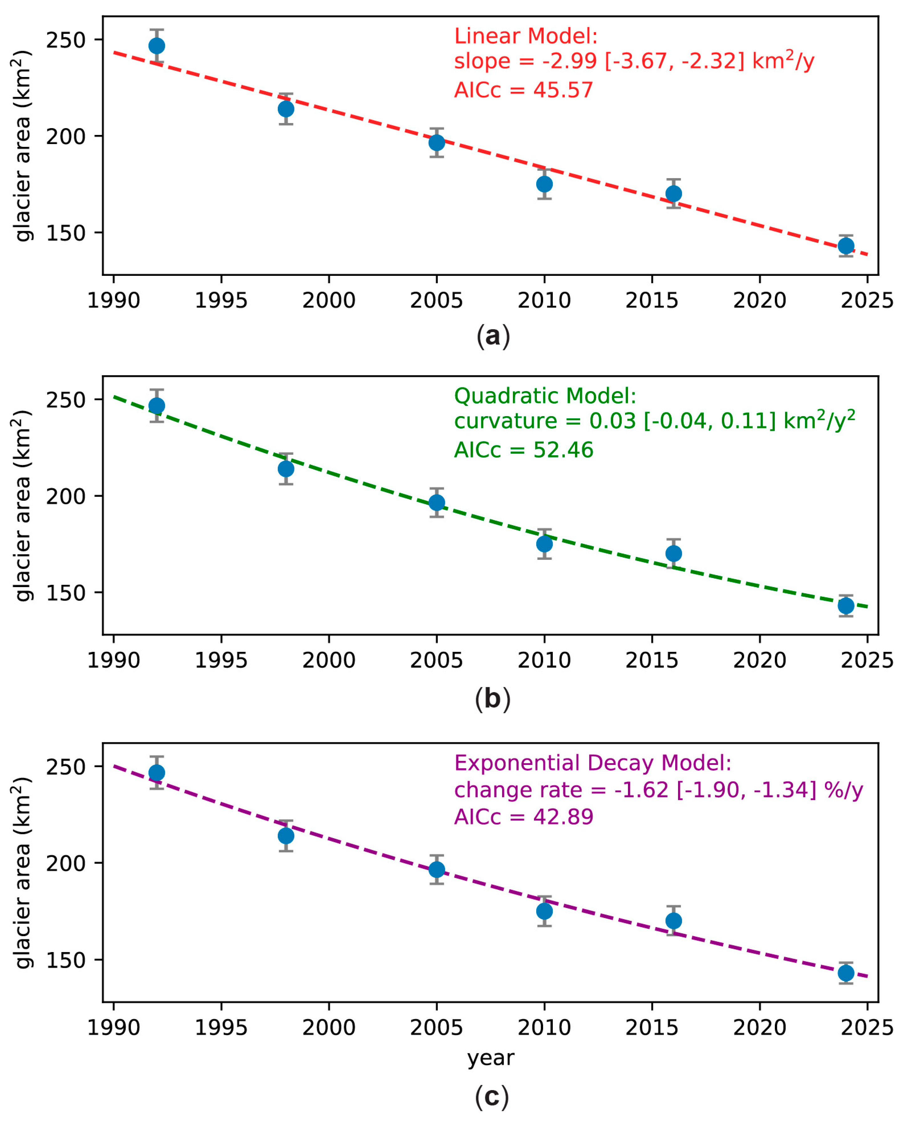
To assess whether there is a detectable acceleration or deceleration in the absolute loss rate, we compare a linear model to a quadratic model for glacier loss (Figure 7a,b). The small-sample corrected Akaike Information Criterion (AICc) value for the linear model is smaller than that for the quadratic model. The difference in AICc values (ΔAICc) between the quadratic and linear models is 6.89, indicating considerably less support for the quadratic model. The estimated quadratic coefficient is small, and its 95% confidence interval (CI) spans both positive and negative values (Figure 7b), indicating that the direction and magnitude of any curvature are poorly constrained by the available observations. Taken together, these results suggest that any acceleration or deceleration in absolute loss rate is not detectable in the available data. Thus, a linear model for the trajectory of glacier loss in the Cordillera Real yields an absolute loss rate of 2.99 km2 yr−1 (95% CI: 2.32 km2 yr−1 to 3.67 km2 yr−1).
We also explore whether a constant fractional loss rate (i.e., exponential decay) can capture the trajectory of glacier loss (Figure 7c). The exponential decay model has a smaller AICc than the linear model. It yields a fractional loss rate of 1.6% yr−1 (95% CI: 1.3% yr−1 to 1.9% yr−1). However, the ΔAICc between the linear and exponential decay models is 2.68, indicating only modestly stronger support for the exponential decay model. Thus, we cannot clearly distinguish between a constant absolute loss rate (i.e., linear model) and a constant fractional loss rate (i.e., exponential decay model). Overall, the glacier retreat in the Cordillera Real between 1992 and 2024 is consistent with a steady long-term decline, with no statistically detectable acceleration or deceleration.

4. Discussion

4.1. Glacier Extent in the Cordillera Real

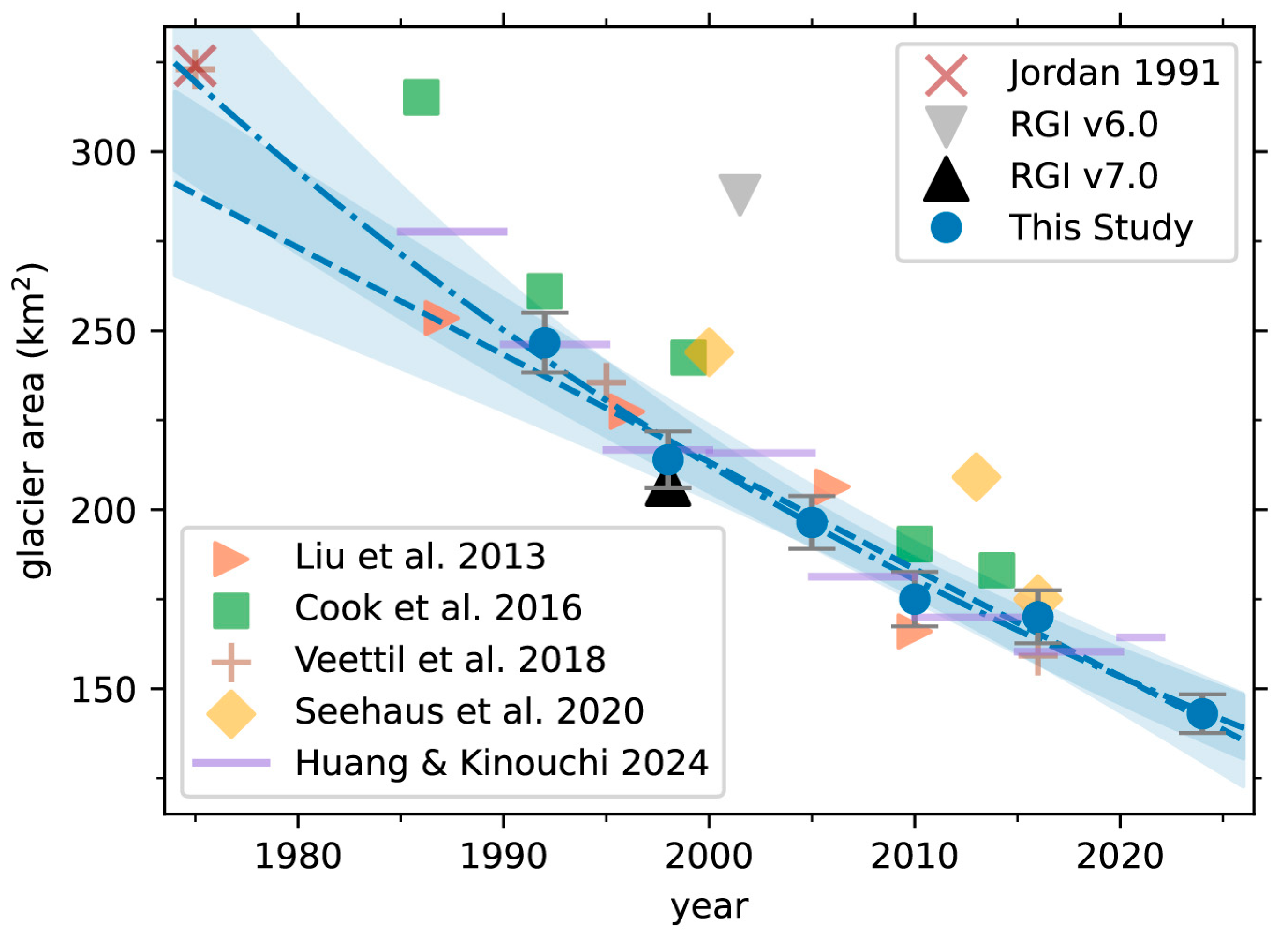
This study provides a time-evolving inventory for glaciers in the Cordillera Real, updating estimates of the glacierized area in recent decades (Figure 8, Table A2). Our estimates generally agree with previous studies, although notable discrepancies occur in the 1980s, around the turn of the century, and in 2013. Our 1992 estimate agrees closely with the 1990–1994 estimate of Huang & Kinouchi (2024) [16] and overlaps with the 10% uncertainty interval for the 1992 estimate of Cook et al. (2016) [14]. Hindcasts from our statistical models suggest that several estimates for the 1980s (e.g., [14,16]) are larger than expected from the long-term trend. In contrast, the 1987 estimate from Liu et al. (2013) [24] is broadly consistent with the linear and exponential-decay trajectories of glacier loss. The 1975 estimates from Jordan (1991) [26] and Veettil et al. (2018) [17] are consistent with an exponential-decay trajectory, but greatly exceed the linear trajectory.
Our 1998 estimate closely matches both the Randolph Glacier Inventory v7.0 estimate for 1998 [22] and the 1995–1999 estimate from Huang & Kinouchi (2024) [16] (Figure 8). However, it is smaller than the turn-of-the-century estimates from Cook et al. (2016) [14], Seehaus et al. (2020) [25], and RGI v6.0 [27]. From the mid-2000s through 2016, our estimates generally agree with previous studies [14,16,17,24,25], with the exception of the 2013 estimate from Seehaus et al. (2020) [25], which exceeds the predictions of our statistical models. Finally, our results indicate continued glacier retreat between 2016 and 2024, in contrast to the slight area increase reported by Huang & Kinouchi (2024) [16] between their 2015–2020 and 2020–2021 estimates.
Differences between our inventory and previous studies may reflect the satellite scenes selected to delineate glacier extents. Many of the largest deviations occur during La Niña years (e.g., the mid-1980s, turn of the century, early 2010s, and early 2020s). These estimates tend to be larger than expected by our long-term trends (Figure 8), likely reflecting greater ephemeral snow cover during cooler and wetter La Niña conditions [11]. In contrast, estimates during El Niño years (e.g., 1975, 1987, 1998, 2010, and 2016) align more closely with the trajectories identified in this study. Differences in methodology may also contribute to the discrepancies. Our use of the composite method from Taylor et al. (2022) [30], together with the inclusion of scenes acquired after the nominal dry season, likely further reduced the influence of ephemeral snow cover. These results suggest that future remote-sensing inventories of outer tropical glaciers would benefit from multi-scene composites, inclusion of a scene acquired after the nominal dry season, and prioritization of imagery from El Niño years.
Our inventory faces some limitations that future studies could address while building on the new data product presented here. Usable satellite scenes prior to 1992 are limited, and we could not implement the annual composite method for earlier years. A multi-year composite approach, similar to that used by Huang & Kinouchi (2024) [16], could allow for the application of a composite method when too few usable scenes are available in a single year. In addition, passive remote-sensing techniques for mapping glacier extents, such as NDSI and band-ratio methods, may not detect debris-covered ice [42], leading to an underestimation of glacier extent. Fortunately, glaciers in the Cordillera Real are predominantly clean ice [14], reducing this source of uncertainty relative to many other mountain regions. However, the three largest relative deviations between our inventory and the RGI v7.0 may result from our inventory’s inability to include debris-covered glacier tongues (Figure A7). Future studies also could incorporate active remote-sensing techniques, such as synthetic-aperture radar, to identify debris-covered glaciers [43]. Our time-evolving inventory (available as shapefiles in the Supplementary Materials) can aid future studies to constrain regional water resources, validate glacier models, and quantify the impacts of glacier loss in the Cordillera Real.

4.2. Glacier Loss in the Cordillera Real

This study provides new insights into the loss of glacierized area in the Cordillera Real. Between 1992 and 2024, we find that 103.67 ± 9.98 km2 of glacierized area has been lost, representing a 42.0 ± 2.1% reduction relative to the 1992 glacierized area. This fractional loss is indistinguishable from the 41.9% loss found by Cook et al. (2016) [14] between 1985 and 2015 and the 42% loss identified by Huang & Kinouchi (2024) [16] between the 1985–1990 and 2015–2020 intervals. Veettil et al. (2018) [17] noted a 50.7% loss over the longer period from 1975 to 2016. Over shorter periods, Seehaus et al. (2020) [25] found a 28% loss between 2000 and 2016, and Liu et al. (2013) [24] identified a 34.5% between 1987 and 2010. To facilitate comparison between studies, we normalized each reported fractional loss by its study duration. Most studies yield an average fractional loss rate of 1.3 ± 0.1% yr−1, relative to the glacierized area of their respective starting years [14,16,17]. Two past studies find notably higher average fractional loss rates, Liu et al. (2013) [24] and Seehaus et al. (2020) [25], with rates of 1.5% yr−1 and 1.8% yr−1, respectively.
The speed at which glacierized areas are vanishing differs between our study and past studies. We find an average absolute loss rate of 3.24 km2 yr−1, which provides a more direct basis for comparison because fractional rates depend on the initial area. This average absolute loss rate is within the 95% confidence interval (CI) of our linear model’s estimate (2.99 [2.32, 3.67] km2 yr−1), but it is 8.4% larger than the central estimate because the 1992 glacierized area in our inventory lies above the fitted trendline (Figure 7a). Our study’s absolute loss rates, however, are smaller than those in past studies. Liu et al. (2013) [24], Huang & Kinouchi (2024) [16], Veettil et al. (2018) [17] found absolute loss rates closest to ours with values of 3.80 km2 y−1, 3.88 km2 y−1, and 3.99 km2 y−1, respectively. However, all three exceed the 95% CI of our linear model slope. The two studies with substantially larger initial glacierized areas than our data had notably larger absolute loss rates of 4.27 km2 yr−1 for Seehau et al. (2020) [25] and 4.33 km2 yr−1 for Cook et al. (2016) [14]. These higher absolute loss rates are consistent with overestimation of the glacierized area early in the study periods (Figure 8), which has been shown to bias estimates of the glacier area loss rates [28,29].
This study refines our understanding of the trajectory of glacier loss in the region. We find no statistical evidence for an acceleration or deceleration in the absolute loss rate (Figure 7), in contrast to several prior studies [16,17,24,25]. This discrepancy likely reflects methodological differences. Many previous studies inferred changes in loss rates by differencing two measurements, whereas we used weighted least squares regression to estimate trend parameters while accounting for measurement uncertainty. Had we relied on two-point differencing, estimated loss rates would have ranged from 5.45 km2 yr−1 (1992–1998) to 0.82 km2 yr−1 (2010–2016), differences that likely reflect ephemeral snow cover and measurement uncertainty rather than changes in the underlying trend. These results underscore the importance of collecting multiple measurements and statistical modeling when evaluating glacier-loss trajectories. However, our small sample size (n = 6 observations) limits our ability to detect subtle departures from linearity or evaluate higher-order models for time-varying loss rates. Future studies could extend the record length and increase the sampling density to improve the statistical power. A similar statistical modeling approach was applied by Cook et al. (2016) [14] for glaciers in the eastern Cordillera of Bolivia, which includes the Cordillera Real. They found a constant fractional loss rate of 2% yr−1, similar to but exceeding the upper bound of our 95% confidence interval for the constant fractional loss rate (1.6 [1.3, 1.9] % yr−1).
Our finding of a constant fractional or absolute loss rate may require reassessing the mechanisms controlling the rate of glacier retreat in the Cordillera Real. Previous studies have attributed changes in loss rates to climate change [17] and El Niño events [25] for acceleration, and to glacier hypsometry [16] for deceleration. However, our results suggest such mechanisms are not required to explain recent changes since we cannot detect a change in the loss rate. A constant fractional loss rate (i.e., exponential decay) can be viewed as a “null” trajectory in which area loss is proportional to the remaining glacierized area. In contrast, a constant absolute loss rate implies that the fractional loss rate increases as the total area declines. For example, an absolute loss of 2.99 km2 yr−1 corresponds to a fractional loss rate of 1.2% yr−1 relative to the 1992 extent but 2.1% yr−1 relative to the 2024 extent. This evolving fractional rate may reflect glacier hypsometry. Glacier loss is concentrated below 5250 m a.s.l., and as retreat has progressed upward, it has affected elevation bands containing a larger fraction of the total glacierized area (Figure 5a), which could sustain a near-constant absolute loss rate. Once lower-elevation glacierized areas (e.g., below ~5500 m) has largely vanished, retreat will occur in elevation bands with progressively less area, and the absolute loss rate should ultimately decline.

4.3. Glacier Longevity in the Cordillera Real

The loss trajectories identified in this study provide first-order scenarios for the evolution of glaciers in the Cordillera Real. Cook et al. (2016) [14] used a similar approach to estimate that about 10% of the 1986 glacierized area in the eastern Cordillera of Bolivia, of which the Cordillera Real is the largest and highest portion, will remain by 2100 CE. Our exponential decay model predicts that about 22% of the glacierized area at our study’s midpoint (2007.5, 188.03 km2) will remain by 2100 CE. Our linear model, in contrast, predicts that the Cordillera Real will deglaciate by the early 2070s CE. However, it is unlikely that glacier loss will continue at a constant absolute rate as retreat becomes concentrated at progressively higher elevations where there is less glacier area (Section 4.2). While these first-order scenarios provide a rough estimate of the longevity of glaciers in the Cordillera Real, their fate will ultimately be determined by the magnitude of future climate change and the hypsometry of the remaining glaciers.
Warming air temperatures in the Cordillera Real have led to increases in regional freezing level heights (FLHs) [21,44]. The FLH helps determine the elevation at which precipitation falls as snow versus rain, affecting both accumulation (snowfall) and ablation (through albedo differences between snow and exposed ice) for outer tropical glaciers [45,46]. FLHs are also positively correlated with equilibrium line altitudes (ELAs) in the Cordillera Real [21,44]. Using WGMS mass-balance data from Zongo Glacier (2012–2021) [31], we estimate an average regional ELA of 5340 ± 10 m a.s.l., nearly 200 m higher than the 5144 ± 67 m estimate for 1991–2006 [33]. Most (71.9%) of the glacierized area loss between 1992 and 2024 occurred below this updated regional ELA, compared with just 31.2% below the earlier estimate for the regional ELA. Future warming will increase ELAs further, with a predicted end-of-century (2100 CE) ELA of 5500 m a.s.l. under an intermediate-emission future (SSP2-4.5) and 5900 m under a high-emission future (SSP5-8.5) [44]. Less than half (46.8%) of the remaining glacierized area is above 5500 m a.s.l., and 58.9% of the remaining glaciers have a maximum elevation below this threshold. A regional ELA of 5900 m a.s.l. would be catastrophic, with 88.6% of the remaining glaciers having a maximum elevation below this value and only 8.4% of the remaining glacierized area above it. Thus, the long-term persistence of glaciers in the Cordillera Real will depend strongly on the magnitude and rate of future warming.

5. Conclusions

This study presents a time-evolving inventory of glaciers in the Cordillera Real from 1992 to 2024 at a spacing of 5 to 8 years. We constructed the inventory to resolve the debate on the trajectory of glacier loss: is it accelerating, decelerating, or continuing at a roughly constant rate? Clarity on the trajectory of glacier loss aids in predictions of their fate. The inventory was built using methods that better capture the extent of glaciers when using remote sensing data and techniques, by limiting the impact of ephemeral snow cover. We used the composite approach from Taylor et al. (2022) [30], including a scene, when possible, from after the nominal dry period, which can better capture glacier extents at outer tropical glaciers [28,29], and focused exclusively on El Niño years. Shapefiles of the glacier extents for the six years in our inventory (1992, 1998, 2005, 2010, 2016, and 2024) are available in the Supplementary Materials section. Key findings are as follows:
  • The Cordillera Real lost 103.67 ± 9.97 km2 of glacierized area in the 32 years between 1992 and 2023, representing a 42.0 ± 2.1% reduction in the area since 1992.
  • There is not a statistically detectable acceleration or deceleration in the absolute (linear model) or fractional (exponential decay) loss rate.
  • Fluctuations in the loss rate calculated between two points likely reflect uncertainty in the measurements or ephemeral snow cover, rather than a change in the loss rate.
  • As a first-order scenario, the constant absolute loss rate (linear) model suggests deglaciation by the early 2070s, and the constant fractional loss rate (exponential decay) model suggests about a fifth (22%) of the glacierized area could remain by 2100 CE.
  • The fate of glaciers in the Cordillera Real will largely depend on how much the future warms, with less than a tenth (8.4%) of the current glacierized area existing above the projected end-of-century (2100 CE) ELA for a high-emissions future (SSP5-8.5) and less than half (46.8%) existing above it for a moderate-emissions future (SSP2-4.5).

Supplementary Materials

The following supporting information can be downloaded at: https://www.mdpi.com/article/10.3390/rs18060905/s1, The time-evolving inventory can be downloaded as ESRI shapefiles.

Author Contributions

Conceptualization, A.G.O.M.; methodology, G.A. and A.G.O.M.; software, G.A. and A.G.O.M.; validation, G.A. and A.G.O.M.; formal analysis, G.A. and A.G.O.M.; investigation, G.A.; resources, G.A. and A.G.O.M.; data curation, G.A. and A.G.O.M.; writing—original draft preparation, G.A.; writing—review and editing, G.A. and A.G.O.M.; visualization, G.A. and A.G.O.M.; supervision, A.G.O.M.; project administration, G.A. and A.G.O.M.; funding acquisition, A.G.O.M. All authors have read and agreed to the published version of the manuscript.

Funding

The material contained in this document is based upon work supported by a National Aeronautics and Space Administration (NASA) grant or cooperative agreement. Any opinions, findings, conclusions, or recommendations expressed in this material are those of the author and do not necessarily reflect the views of NASA. This work was supported through a NASA grant awarded to the Illinois/NASA Space Grant Consortium.

Data Availability Statement

Version 7.0 of the Randolph Glacier Inventory can be accessed at https://www.glims.org/RGI/ (accessed on 14 May 2025). The SRTM GL1 DEM can be accessed at https://opentopography.org/ (accessed on 14 May 2025). Landsat scenes can be accessed from the United States Geological Survey at https://earthexplorer.usgs.gov/ (accessed on 15 May 2025) or through Google Earth Engine at https://earthengine.google.com/ (accessed on 15 May 2025). World Glacier Monitoring Service mass balance data can be accessed at https://wgms.ch/ (accessed on 1 June 2025).

Acknowledgments

The authors thank two anonymous reviewers for their detailed and constructive comments and suggestions that greatly improved the soundness and presentation of the article.

Conflicts of Interest

The authors declare no conflicts of interest.

Abbreviations

The following abbreviations are used in this manuscript:
ELAEquilibrium line altitude
RGIRandolph glacier inventory
m.a.s.lMeters above sea level
AICAkaike information criterion
ENSOEl Niño Southern Oscillation
SRTMShuttle Radar Topography Mission
DEMDigital Elevation Model
QGISQuantum Geographic Information System
NDSINormalized Difference Snow Index
NDWINormalized Difference Water Index

Appendix A

To assess the impact of our threshold values in the glacier-mapping algorithm (Section 2.2), we conducted a sensitivity analysis. We estimated the glacierized area in 2024 using three NDSI thresholds: (1) 0.45, (2) 0.5 (used in this study), and (3) 0.55. The NDSI threshold of 0.45 leads to the largest area, and the NDSI threshold of 0.55 leads to the smallest area (Table A1). However, these end-member area estimates overlap in their 2–σ uncertainties. While the three area estimates are indistinguishable (statistically), visual inspection of the resulting glacier masks finds that an NDSI value of 0.45 tends to include areas in shadow that are not glacierized, and the NDSI value of 0.55 often excludes portions of the ablation zone. The NDSI threshold of 0.5 balances these two biases well and thus requires the least manual post-processing to accurately map glacier extents.
Table A1. Glacier area and area uncertainty (in km2) in 2024 based on just the NDSI and the NDSI with lake removal and manual editing (This Study).
VersionArea [km2]Uncertainty [km2]
NDSI > 0.45150.866.55
NDSI > 0.50146.895.60
NDSI > 0.55142.915.52
This Study143.005.41
We also assessed the impact of our lake-removal algorithm and manual edits by comparing the estimated glacierized area based on just the NDSI threshold of 0.50 to the value we found in this study for 2024, which includes an NDSI threshold of 0.50 as well as these additional steps. The glacier area after lake removal and edits is smaller but statistically indistinguishable from the area using just the NDSI threshold (Table A1). Almost a third (32.1%) of the reduction in glacier area comes from removing proglacial lakes (1.25 ± 0.15 km2). Removing proglacial lakes is necessary since many have formed and grown as the glaciers have retreated [14,16]. The remaining difference in area largely results from manually adjusting the glacier boundaries in shadowed regions, but this difference is less than half of the uncertainty associated with the area estimates.

Appendix B

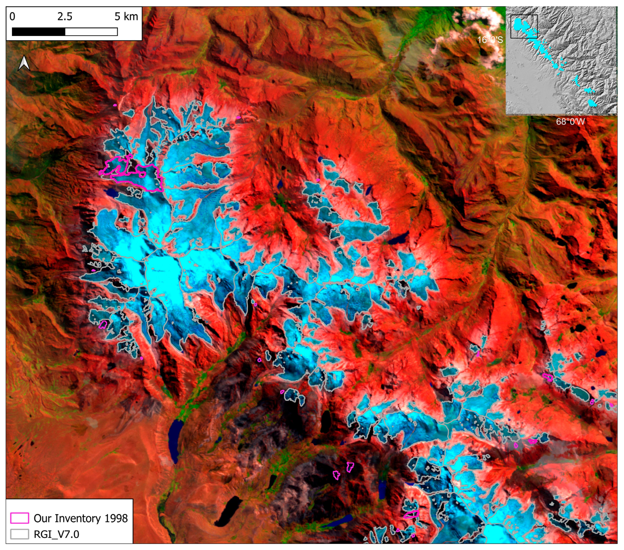
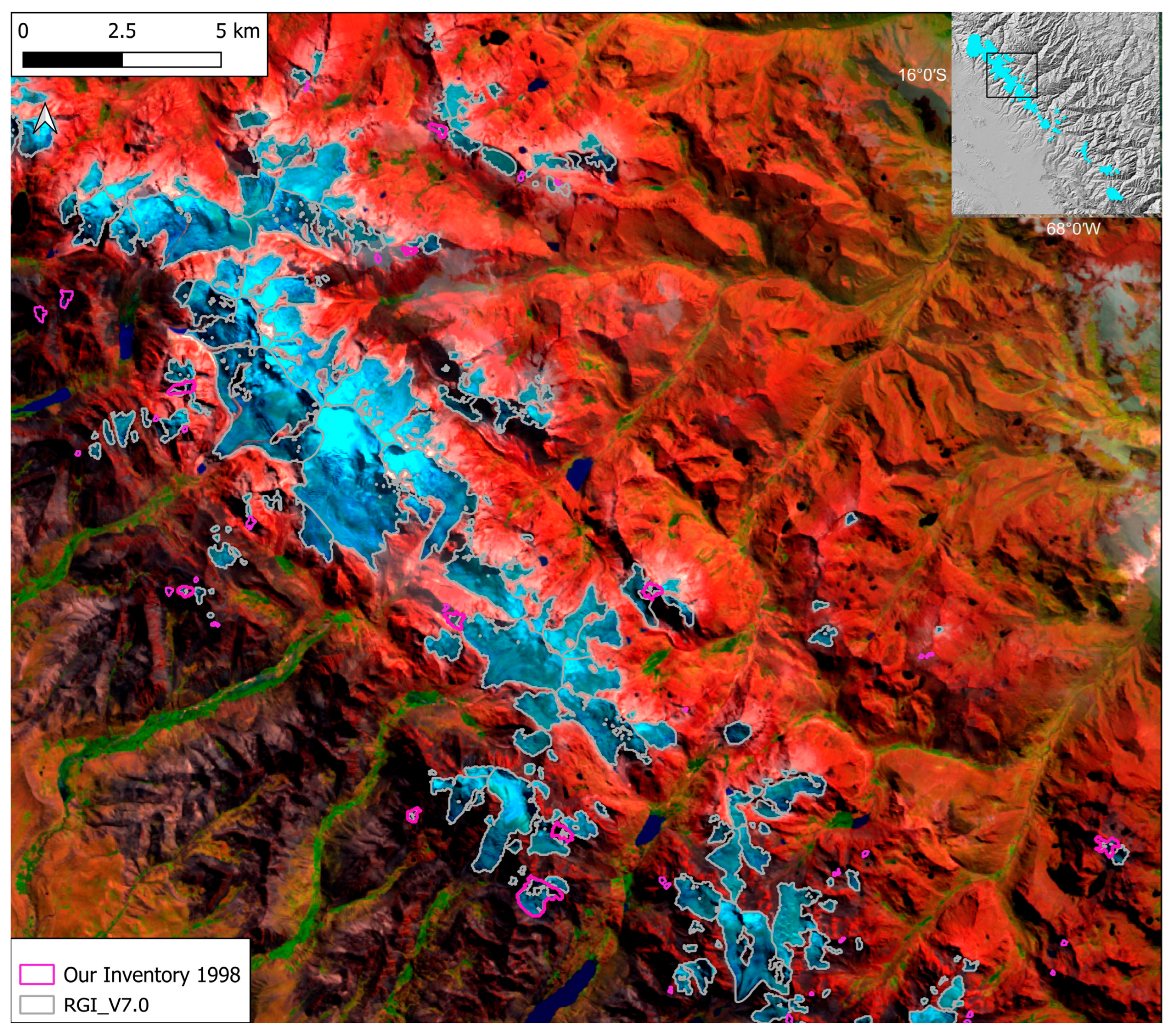
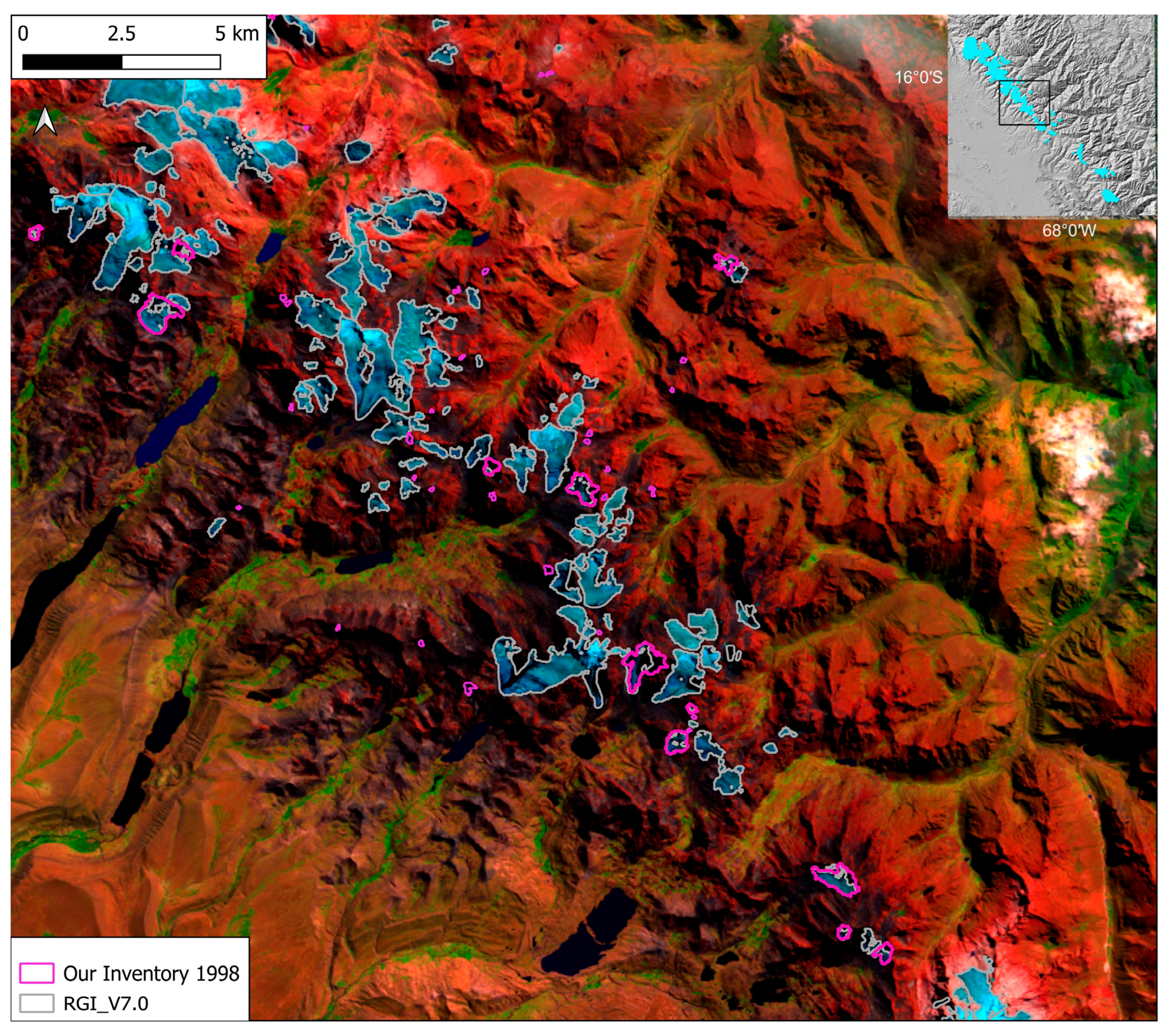
To further compare our inventory to the RGI v7.0, we analyzed the size difference between the 485 glacier basins common to both inventories (Figure A1). While there is a slight left-skew to the distributions, especially when viewed as a relative area difference (Figure A1b), most areas of the glacier basins in our inventory are statistically indistinguishable from their values in the RGI 7.0. Of the 485 common glacier basins, 446 basins (92.0%) have an area in the RGI v.7.0 that falls within the 2–σ uncertainty of the area estimate for that basin in our inventory. We also visually compare our inventory to the RGI v.7.0, highlighting the 39 basins whose areas are statistically distinguishable between inventories and the 82 glaciers in our inventory not found in the RGI v. 7.0 (Figure A2, Figure A3, Figure A4, Figure A5, Figure A6 and Figure A7). Three glaciers are multiple factors smaller in our inventory than in the RGI (Figure A1), which are located south of Illimani (Figure A7), and likely have debris-covered tongues, which cannot be mapped using our remote sensing techniques.
Figure A1. Difference in absolute (a) and relative (b) glacier area in our inventory versus the RGI v.7.0 for the 485 glacier basins that are common to both inventories. Differences are said to be significant if they exceed the 2–σ uncertainty of the area estimate for that basin in our inventory.
Remotesensing 18 00905 g0a1
Figure A2. Comparison of glacier basins between our inventory and the RGI v.7.0 for the northern-most section of the Cordillera Real. Glacier extents from the RGI v.7.0 are shown in gray. Glacier extents from our inventory are only shown in magenta for those basins with statistically distinguishable area differences between inventories. Included in the magenta extents are those glaciers in our inventory that are not also included in the RGI v.7.0. The black box in the insert map of the Cordillera Real indicates the map area.
Remotesensing 18 00905 g0a2
Figure A3. Same as Figure A2 but for a more southernly section of the Cordillera Real.
Remotesensing 18 00905 g0a3
Figure A4. Same as Figure A3 but for a more southernly section of the Cordillera Real.
Remotesensing 18 00905 g0a4
Figure A5. Same as Figure A4 but for a more southernly section of the Cordillera Real.
Remotesensing 18 00905 g0a5
Figure A6. Same as Figure A5 but for a more southernly section of the Cordillera Real.
Remotesensing 18 00905 g0a6
Figure A7. Same as Figure A6 but for the southern-most section of the Cordillera Real.
Remotesensing 18 00905 g0a7

Appendix C

The area and count of the glaciers in our time-evolving inventory can be found in Table A2 and Table A3, respectively. The glacier area has a clear downward trend for the entire Cordillera Real and each size category (Table A2). The evolution in the number of glacier basins (i.e., count) has a trend that is less clear (Table A3). As larger glaciers shrink, they can be reclassified as smaller glaciers. Also, many glacier basins that were considered a single basin earlier in the study period have since separated into multiple smaller basins. Thus, if a medium glacier both shrinks and separates into multiple basins, then it would account for one loss in the medium glacier category but multiple gains to the small glacier category.
Table A2. Glacier area ± 2–σ uncertainty (in km2) for the six years of our time-evolving inventory, presented as both the total and for the various size bins in this study.
Glacier Size199219982005201020162024
Small62.32 ± 0.9352.39 ± 0.9448.16 ± 0.8841.11 ± 0.8340.47 ± 0.8035.36 ± 0.78
Medium152.63 ± 1.59130.18 ± 1.67124.99 ± 1.63121.06 ± 1.76116.86 ± 1.7295.44 ± 1.56
Large31.73 ± 0.7930.38 ± 0.8623.30 ± 0.5712.83 ± 0.3712.74 ± 0.3712.20 ± 0.42
Total246.67 ± 8.37213.96 ± 7.93196.45 ± 7.35175.01 ± 7.58170.08 ± 7.40143.00 ± 5.41
Table A3. Glacier count for the six years of our time-evolving inventory, presented as both the total and for the various size bins in this study.
Glacier Size199219982005201020162024
Small533467467473423435
Medium1179892868372
Large554222
Total655570563561508509

References

  1. Kaser, G. A review of the modern fluctuations of tropical glaciers. Glob. Planet. Chang. 1999, 22, 93–103. [Google Scholar] [CrossRef] [Scilit]
  2. Kaser, G.; Osmaston, H. Tropical Glaciers; Cambridge University Press: Cambridge, UK, 2002. [Google Scholar]
  3. Vuille, M.; Francou, B.; Wagnon, P.; Juen, I.; Kaser, G.; Mark, B.G.; Bradley, R.S. Climate change and tropical Andean glaciers: Past, present and future. Earth-Sci. Rev. 2008, 89, 79–96. [Google Scholar] [CrossRef] [Scilit]
  4. Brecher, H.H.; Thompson, L.G. Measurement of the retreat of Qori Kalis Glacier, Peru, by terrestrial photogrammetry. Photogramm. Eng. Remote Sens. 1993, 59, 1017–1022. [Google Scholar]
  5. Ames, A.; Francou, B. Cordillera Blanca – Glaciares en al historia. Bull. L’institut Français D’études Andin. 1995, 24, 37–64. [Google Scholar] [CrossRef] [Scilit]
  6. Hastenrath, S.; Ames, A. Diagnosing the imbalance of of Yanamarey Glacier in the Cordillera Blanca of Peru. J. Geophys. Res. 1995, 100, 5105–5112. [Google Scholar] [CrossRef] [Scilit]
  7. Hastenrath, S.; Ames, A. Recession of Yanamarey Glacier in Cordillera Blanca, Peru. J. Glaciol. 1995, 41, 127–133. [Google Scholar] [CrossRef] [Scilit]
  8. Francou, B.; Vuille, M.; Wagnon, P.; Mendoza, J.; Sicart, J. Tropical climate change recorded by a glacier in the central Andes during the last decades of the twentieth century: Chacaltaya, Bolivia, 16°S. J. Geophys. Res. Atmos. 2003, 108, 4154. [Google Scholar] [CrossRef] [Scilit]
  9. Ramírez, E.; Francou, B.; Ribstein, P.; Descloitres, M.; Guérin, R.; Mendoza, J.; Gallaire, R.; Pouyaud, B.; Jordan, E. Small glaciers disappearing in the tropical Andes: A case-study in Bolivia: Glaciar Chacaltaya (16° S). J. Glaciol. 2001, 47, 187–194. [Google Scholar] [CrossRef] [Scilit]
  10. Soruco, A.; Vincent, C.; Francou, B.; Gonzalez, J.F. Glacier decline between 1963 and 2006 in the Cordillera Real, Bolivia. Geophys. Res. Lett. 2009, 36, L03502. [Google Scholar] [CrossRef] [Scilit]
  11. Rabatel, A.; Francou, B.; Soruco, A.; Gomez, J.; Cáceres, B.; Ceballos, J.L.; Basantes, R.; Vuille, M.; Sicart, J.-E.; Huggel, C.; et al. Current state of glaciers in the tropical Andes: A multi-century perspective on glacier evolution and climate change. Cryosphere 2013, 7, 81–102. [Google Scholar] [CrossRef] [Scilit]
  12. Vergara, W.; Deeb, A.; Valencia, A.; Bradley, R.; Francou, B.; Zarzar, A.; Grünwaldt, A.; Haeussling, S. Economic impacts of rapid glacier retreat in the Andes. Eos 2007, 88, 261–268. [Google Scholar] [CrossRef] [Scilit]
  13. Ribstein, P.; Tiriau, E.; Francou, B.; Saravia, R. Tropical climate and glacier hydrology: A case study in Bolivia. J. Hydrol. 1995, 165, 221–234. [Google Scholar] [CrossRef] [Scilit]
  14. Cook, S.J.; Kougkoulos, I.; Edwards, L.A.; Dortch, J.; Hoffmann, D. Glacier change and glacial lake outburst flood risk in the Bolivian Andes. Cryosphere 2016, 10, 2399–2413. [Google Scholar] [CrossRef] [Scilit]
  15. Hanshaw, M.N.; Bookhagen, B. Glacial areas, lake areas, and snow lines from 1975 to 2012: Status of the Cordillera Vilcanota, including the Quelccaya Ice Cap, northern central Andes, Peru. Cryosphere 2014, 8, 359–376. [Google Scholar] [CrossRef] [Scilit]
  16. Huang, Y.; Kinouchi, T. Revealing decadal glacial changes and lake evolution in the Cordillera Real, Bolivia: A semi-automated Landsat imagery analysis. Remote Sens. 2024, 16, 1231. [Google Scholar] [CrossRef] [Scilit]
  17. Veettil, B.K.; Wang, S.; Simões, J.C.; Pereira, S.F.R. Glacier monitoring in the eastern mountain ranges of Bolivia from 1975 to 2016 using Landsat and Sentinel-2 data. Environ. Earth Sci. 2018, 77, 452. [Google Scholar] [CrossRef] [Scilit]
  18. Soruco, A.; Vincent, C.; Rabatel, A.; Francou, B.; Thibert, E.; Sicart, J.E.; Condom, T. Contribution of glacier runoff to water resources of La Paz city, Bolivia (16° S). Ann. Glaciol. 2015, 56, 147–154. [Google Scholar] [CrossRef] [Scilit]
  19. Kaser, G.; Großhauser, M.; Marzeion, B. Contribution potential of glaciers to water availability in different climate regimes. Proc. Natl. Acad. Sci. USA 2010, 107, 20223–20227. [Google Scholar] [CrossRef] [Scilit]
  20. Saberi, L.; McLaughlin, R.T.; Ng, G.-H.C.; La Frenierre, J.; Wickert, A.D.; Baraer, M.; Zhi, W.; Li, L.; Mark, B.G. Multi-scale temporal variability in meltwater contributions in a tropical glacierized watershed. Hydrol. Earth Syst. Sci. 2019, 23, 405–425. [Google Scholar] [CrossRef] [Scilit]
  21. Vuille, M.; Carey, M.; Huggel, C.; Buytaert, W.; Rabatel, A.; Jacobsen, D.; Soruco, A.; Villacis, M.; Yarlequé, C.; Elison Timm, O.; et al. Rapid decline of snow and ice in the tropical Andes – Impacts, uncertainties and challenges ahead. Earth-Sci. Rev. 2018, 176, 195–213. [Google Scholar] [CrossRef] [Scilit]
  22. RGI 7.0 Consortium. Randolph Glacier Inventory—A Dataset of Global Glacier Outlines, 7th ed.; NSIDC (National Snow and Ice Data Center): Boulder, CO, USA, 2023. [Google Scholar] [CrossRef]
  23. NASA Shuttle Radar Topography Mission (SRTM). Shuttle Radar Topography Mission (SRTM) Global; OpenTopography: San Diego, CA, USA, 2013. [Google Scholar] [CrossRef]
  24. Liu, T.; Kinouchi, T.; Ledezma, F. Characterization of recent glacier decline in the Cordillera Real by LANDSAT, ALOS, and ASTER data. Remote Sens. Environ. 2013, 137, 158–172. [Google Scholar] [CrossRef] [Scilit]
  25. Seehaus, T.; Malz, P.; Sommer, C.; Soruco, A.; Rabatel, A.; Braun, M. Mass balance and area changes of glaciers in the Cordillera Real and Tres Cruces, Bolivia, between 2000 and 2016. J. Glaciol. 2020, 66, 124–136. [Google Scholar] [CrossRef] [Scilit]
  26. Jordan, E. Die Gletscher der Bolivianischen Anden: Eine Photogrammetrisch-Kartographische Bestandsaufnahme der Gletscher Boliviens Als Grundlage für Klimatische Deutungen und Potential für die Wirtschaftliche Nutzung; Steiner: Stuttgart, Germany, 1991. [Google Scholar]
  27. RGI Consortium. Randolph Glacier Inventory—A Dataset of Global Glacier Outlines, 6th ed.; NSIDC (National Snow and Ice Data Center): Boulder, CO, USA, 2017. [Google Scholar] [CrossRef]
  28. Kochtitzky, W.H.; Edwards, B.R.; Enderlin, E.M.; Marino, J.; Marinque, N. Improved estimates of glacier change rates at Nevado Coropuna Ice Cap, Peru. J. Glaciol. 2018, 64, 175–184. [Google Scholar] [CrossRef] [Scilit]
  29. Malone, A.G.O.; Broglie, E.T.; Wrightsman, M. The evolution of the two largest tropical ice masses since the 1980s. Geosciences 2022, 12, 365. [Google Scholar] [CrossRef] [Scilit]
  30. Taylor, L.S.; Quincey, D.J.; Smith, M.W.; Potter, E.R.; Castro, J.; Fyffe, C.L. Multi-decadal glacier area and mass balance change in the southern Peruvian Andes. Front. Earth Sci. 2022, 10, 863933. [Google Scholar] [CrossRef] [Scilit]
  31. WGMS. Fluctuations of Glaciers (FoG) Database; World Glacier Monitoring Service (WGMS): Zurich, Switzerland, 2025. [Google Scholar] [CrossRef]
  32. Cuffey, K.M.; Paterson, W.S.B. The Physics of Glaciers, 4th ed.; Elsevier: Burlington, MA, USA, 2010. [Google Scholar]
  33. Rabatel, A.; Bermejo, A.; Loarte, E.; Soruco, A.; Gomez, J.; Leonardini, G.; Vincent, C.; Sicart, J.E. Can the snowline be used as an indicator of the equilibrium line and mass balance for glaciers in the outer tropics? J. Glaciol. 2012, 58, 1027–1036. [Google Scholar] [CrossRef] [Scilit]
  34. Hall, D.K.; Riggs, G.A.; Salomonson, V.V. Development of methods for mapping global snow cover using MODIS data. Remote Sens. Environ. 1995, 54, 127–140. [Google Scholar] [CrossRef] [Scilit]
  35. Huggel, C.; Kääb, A.; Haeberli, W.; Teysseire, P.; Paul, F. Remote sensing based assessment of hazards from glacier lake outbursts: A case study in the Swiss Alps. Can. Geotech. J. 2002, 39, 316–330. [Google Scholar] [CrossRef] [Scilit]
  36. Paul, F.; Bolch, T.; Briggs, K.; Kääb, A.; McMillan, M.; McNabb, R.; Nagler, T.; Nuth, C.; Rastner, P.; Strozzi, T.; et al. Error sources and guidelines for quality assessment of glacier area, elevation change, and velocity products derived from satellite data in the Glaciers_cci project. Remote Sens. Environ. 2017, 203, 256–275. [Google Scholar] [CrossRef] [Scilit]
  37. Seabold, S.; Perktold, J. Statsmodels: Econometric and statistical modeling with Python. In Proceedings of the 9th Python in Science Conference, Austin, TX, USA, 28 June–3 July 2010; pp. 57–61. [Google Scholar] [CrossRef] [Scilit]
  38. Akaike, H. Information Theory and an Extension of the Maximum Likelihood Principle. In Second International Symposium on Information Theory; Petrov, B.N., Csáki, F., Eds.; Akademiai Kiado: Budapest, Hungary, 1973; pp. 267–281. [Google Scholar]
  39. Sugiura, N. Further analysis of the data by Akaike’s information criterion and the finite corrections. Commun. Stat.-Theory Methods 1978, 7, 13–26. [Google Scholar] [CrossRef] [Scilit]
  40. Hurvich, C.M.; Tsai, C.L. Regression and time series model selection in small samples. Biometrika 1989, 76, 297–307. [Google Scholar] [CrossRef]
  41. Portet, S. A primer on model selection using the Akaike Information Criterion. Infect. Dis. Model. 2020, 5, 111–128. [Google Scholar] [CrossRef] [Scilit]
  42. Racoviteanu, A.E.; Paul, F.; Raup, B.; Khalsa, S.J.S.; Armstrong, R. Challenges and recommendations in mapping of glacier parameters from space: Results of the 2008 Global Land Ice Measurements from Space (GLIMS) workshop, Boulder, Colorado, USA. Ann. Glaciol. 2009, 50, 53–69. [Google Scholar] [CrossRef] [Scilit]
  43. Atwood, D.K.; Meyer, F.; Arendt, A. Using L-band SAR coherence to delineate glacier extent. Can. J. Remote Sens. 2010, 36, S186–S195. [Google Scholar] [CrossRef] [Scilit]
  44. Turner, S.A.; Vuille, M.; Rabatel, A. Constraining future projections of freezing level height and equilibrium-line altitudes in the tropical Andes based on CMIP6. J. Geophys. Res. Atmos. 2025, 130, e2024JD042963. [Google Scholar] [CrossRef] [Scilit]
  45. Schauwecker, S.; Rohrer, M.; Acuña, D.; Cochachin, A.; Dávila, L.; Frey, H.; Giráldez, C.; Gómez, J.; Huggel, C.; Jacques-Coper, M.; et al. Climate trends and glacier retreat in the Cordillera Blanca, Peru, revisited. Glob. Planet. Chang. 2014, 119, 85–97. [Google Scholar] [CrossRef] [Scilit]
  46. Schauwecker, S.; Rohrer, M.; Huggel, C.; Endries, J.; Montoya, N.; Neukom, R.; Perry, B.; Salzmann, N.; Schwarb, M.; Suarez, W. The freezing level in the tropical Andes, Peru: An indicator for present and future glacier extents. J. Geophys. Res. Atmos. 2017, 122, 5172–5189. [Google Scholar] [CrossRef] [Scilit]
Figure 1. Map of Bolivia noting the location of the glaciers in the Cordillera Real (black box). Blue polygons indicate glacier extents based on the RGI v7.0 [22]. The inset map of South America indicates the map area in red. The background map is the 30 m SRTM digital elevation model [23].
Remotesensing 18 00905 g001
Figure 2. Estimates of glacierized area in the Cordillera Real over time from five past studies [14,16,17,24,25] and three glacier inventories [22,26,27].
Remotesensing 18 00905 g002
Figure 3. Glacier mapping algorithm displaying a (a) false color composite of a glacierized section of the Cordillera Real, (b) pixels identified as snow or ice by the NDSI, (c) pixels identified as water by the NDWI, and (d) the finalized glacierized area outlined in white after removing proglacial lakes and manual post-processing. The red box in the right-most figure indicates the location of the glacierized section in (a) through (d).
Remotesensing 18 00905 g003
Figure 4. Glacier extents in 1992 and 2024 for the (a) northern portion of the Cordillera Real and (b) the southern portion. The pink boxes in the insert map indicate the two portions. The background map in (a) and (b) is a hillshade of the 30 m SRTM DEM [23].
Remotesensing 18 00905 g004
Figure 5. Distribution of the glacierized area in the Cordillera Real for 1992 and 2024 by (a) elevation and (c) aspect. Relative area loss between 1992 and 2024 by (b) elevation and (d) aspect.
Remotesensing 18 00905 g005
Figure 6. (a) Absolute and (b) relative glacier area loss from 1992 to 2024 (dot color) with respect to size (marker size), median elevation (distance from center), and aspect (angle) for the 570 glaciers in the Cordillera Real. Gray marks indicate glaciers whose area change is smaller than the associated 2–σ uncertainty. The bolded black line at 5340 m a.s.l. denotes the recent ELA at Zongo glacier. Lower elevations are toward the outside.
Remotesensing 18 00905 g006
Figure 7. (a) Linear, (b) quadratic, and (c) exponential decay models of glacier loss. Models are noted by dashed lines. Glacier area data with 2–σ uncertainties are noted by the blue dots with error bars. The small-sample corrected Akaike Information Criterion (AICc) is noted for each model, as well as the value of the model’s key parameter.
Remotesensing 18 00905 g007
Figure 8. Temporal evolution of glacier area changes in the Cordillera Real for this study compared with previous studies [14,16,17,24,25] and three glacier inventories [22,26,27]. The blue lines in the plot are the trajectories of the linear (dashed line) and exponential decay models (dot-dashed line), with the shading noting their 95% confidence intervals.
Remotesensing 18 00905 g008
Table 1. Date, location, and sensor for the Landsat scenes used in this study.
YearMonthDayPathRowSensor

1992
May
November
December
25
3
21

001

071

LT05

1998
May
June
September
12
13
17

001

071

LT05

2005
June
August
September
16
3
4

001

071

LT05

2010
June
August
November
14
17
5

001

071

LT05

2016
May
August
September
29
17
18

001

071

LT05

2024
June
September
October
3
8
2

001

071
LC08
LC08
LC09
Table 2. Glacier count and area for the RGI v7.0 and count and area ± 2σ uncertainty for this study’s 1998 inventory.
RGI v7.0Our Inventory, 1998
Glacier SizeCountArea [km2]CountArea [km2]
Small39050.2746753.39 ± 0.94
Medium92126.6898130.18 ± 1.67
Large530.37530.39 ± 0.86
Total487207.32570213.96 ± 7.93
Disclaimer/Publisher’s Note: The statements, opinions and data contained in all publications are solely those of the individual author(s) and contributor(s) and not of MDPI and/or the editor(s). MDPI and/or the editor(s) disclaim responsibility for any injury to people or property resulting from any ideas, methods, instructions or products referred to in the content.