Highlights
What are the main findings?
- The microwave radiative transfer model can capture subtle variations of magnetic field parameters.
- Updating oxygen parameters and Zeeman splitting coefficients in the microwave LBL model can improve oxygen absorption line simulation accuracy.
What are the implications of the main findings?
- Observed magnetic field parameters, particularly capable of reflecting magnetic field sudden change information, should be widely utilized in upper atmospheric microwave radiative transfer simulations and applications.
- Accurate modeling of the fine-structure of oxygen absorption lines enhances spectral analysis effectiveness, contributing to advancements in microwave sounder channel parameter design, data assimilation, and retrieval.
Abstract
The upper atmospheric microwave sounding channels data are important for atmospheric data assimilation and retrieval. However, radiative transfer simulation accuracy is constrained by the precise characterization of the Zeeman splitting effect. This study investigates key influencing factors in upper-atmospheric microwave radiance simulations, focusing on the geomagnetic field parameters and the Zeeman splitting absorption coefficients. A three-dimensional (3D) atmosphere-magnetic coupling dataset is constructed using the Sounding of the Atmosphere using Broadband Emission Radiometry (SABER) version 2.0 Level 2A atmospheric profiles and the International Geomagnetic Reference Field (IGRF-13) as input for the microwave Line-by-Line (LBL) model. Observations from Special Sensor Microwave Imager/Sounder (SSMIS) channels 19 and 20 are used to quantitatively compare the effects of 2D and 3D geomagnetic fields on simulations and evaluate the impact of updated Zeeman splitting coefficients. Quantitative analysis reveals that the average vertical attenuation rate of geomagnetic field strength between 50 and 0.001 hPa is 2.98%, and using 3D magnetic field parameters improves the observation and simulation bias (O-B) for SSMIS channels 19 and 20 by approximately 3.67% and 3.52%, respectively. The updated microwave LBL model, incorporating molecular self-spin interactions and higher-order Zeeman effects, reduces the mean absolute error (MAE) and root mean square error (RMSE) of the SSMIS channel 20 by approximately 2.7% and 2.25%, respectively. Experimental results indicate that the 7+ line within a 2 MHz frequency shift is sensitive to moderate magnetic field strength (0.35–0.55 Gauss), while the 1− line is sensitive to strong magnetic fields (0.5–0.7 Gauss). This study demonstrates that optimizing geomagnetic field representation and Zeeman splitting coefficients can improve upper atmospheric microwave radiance simulation accuracy by detailed comparison with observations.
1. Introduction
Accurate observations and simulations of atmospheric temperatures are key for numerical weather prediction (NWP) and long-term climate analysis [1,2,3]. Incorporating upper atmospheric observations into NWP systems not only helps in understanding atmospheric dynamic processes but also directly enhances the stratosphere and mesosphere atmospheric state forecasts [4,5,6,7,8]. Satellite observations have become one of the most important data sources for global NWP data assimilation systems due to their global coverage, high temporal and spatial resolution, and superior data consistency. Spaceborne microwave sounder observations exhibit high sensitivity to atmospheric temperature, playing an irreplaceable role in the NWP system [9]. Based on research of the oxygen spectral emission and absorption characteristics in the microwave band, passive remote sensing of atmospheric temperature can be achieved [10]. Systematically investigating the factors that influence oxygen (O2) absorption line simulations helps to improve radiative transfer model accuracy. This provides theoretical support for upper-atmospheric temperature detection and the application of satellite observations. Ref. [11] conducted a comparative study between observations from the Millimeter-wave Atmospheric Sounder (MAS) and simulations from the Zeeman Propagation Model (ZPM). This research first confirmed the selective response of oxygen fine-structure line brightness temperature (BT) to atmospheric temperature at specific altitudes by comparing with observations. Specifically, by combining the observations of 25+ (65.7648 GHz), 9+ (61.1506 GHz), and 1− (118.7503 GHz) O2 absorption lines, atmospheric temperatures at approximately 60 km, 80 km, and 95 km altitude can be retrieved, respectively. This experiment provides a key technical pathway for continuous temperature detection in the middle and upper atmosphere [11].
The interaction between an external magnetic field and the magnetic moment of a molecule or atom causes energy level splitting, resulting in spectral line splitting. This effect is known as Zeeman splitting [12]. For microwave oxygen absorption channels, the influence of the Earth’s magnetic field will affect their observation and simulation above 40 km [13]. The physical mechanism involves competition between pressure broadening and the Zeeman splitting effect of oxygen spectral lines. Specifically, the frequency shift caused by pressure broadening far exceeds the Zeeman splitting at lower atmosphere, covering the Zeeman splitting fine structure, and its details are unobservable. However, when the altitude exceeds 40 km, atmospheric pressure drops sharply, causing the pressure broadening gradually diminish until it becomes comparable or even smaller than the Zeeman splitting effect. At this condition, the magnetic field becomes the dominant factor determining spectral line structure and radiation characteristics [10].
By comparing observations with simulations, the impact of the vertical distribution of the Earth’s magnetic field on the microwave radiative transfer model (RTM) simulations in the upper atmosphere can be quantified. Ref. [14] indirectly analyzed the impact of three-dimensional (3D) and two-dimensional (2D) geomagnetic fields on the Special Sensor Microwave Imager/Sounder (SSMIS) channel 19–22 simulations through the Atmospheric Radiative Transfer Simulator (ARTS) and the Radiative Transfer for the TIROS Operational Vertical Sounder (RTTOV). The study utilized the Met Office global NWP model atmospheric profiles as input. However, these profiles are only up to 10 hPa (approximately 65 km), with temperatures above 10 hPa set to be consistent. Since the SSMIS channels 19 and 20 peak in the weighting function occurs between 60 and 80 km, their observed signals primarily originate from the upper atmosphere. The assumption of constant temperature leads to significant biases between the simulations of these two channels and the real atmospheric state, making it impossible to compare with satellite observations. The detection altitude of channels 21 and 22 is relatively lower than that of channels 19 and 20 (primarily covering 40–65 km), demonstrating good consistency between their simulations and observations. This provides a reliable foundation for analyzing the influence of magnetic field dimensions. Results indicate that the influence of Earth’s magnetic field dimensions on simulation accuracy exhibits significant channel dependence. When ARTS employs a 3D geomagnetic field, the simulation bias increases significantly compared to 2D. The standard deviation for channel 19 rises from 0.33 K to 1.8 K, with equatorial variations reaching ±7 K. This demonstrates that the 3D structure of the magnetic field critically impacts RTM simulations in the upper atmosphere at low latitudes. However, unidentified systematic biases persist between the models employed in this study, which are likely to interfere with the quantitative analysis of magnetic field dimensions [14].
Extensive research has employed sensitivity analysis of the magnetic field dependence of O2 fine-structure lines to investigate the impact of external magnetic fields on upper atmospheric microwave observations and simulations [10,11,15,16]. However, most of these studies were conducted at the end of the last century. The limitations of earlier research have gradually become apparent as the O2 parameter databases and Zeeman splitting computational models continue to be updated [17,18]. The most notable is that early microwave Line-by-Line (LBL) models are largely based on the pure Hund’s case (b) coupling assumption. This assumption neglects molecular self-spin interactions and higher-order Zeeman effects, leading to simulation limitations when oxygen molecules have low-energy levels (), which can cause simulation errors up to 10 K [17]. Reference [17] updated the Zeeman splitting coefficient database. By employing more accurate and detailed computational methods, the simulation accuracy of oxygen fine-structure lines has been significantly improved, particularly for lines with low . This improvement not only significantly impacts microwave RTM simulations but also provides a more reliable foundation for atmospheric temperature and magnetic field retrieval studies.
In Section 2, the atmospheric and geomagnetic field profiles used in this study are systematically described, as well as the microwave LBL model developed by Rosenkranz and Staelin (hereafter referred to as RS-LBL), which can accurately simulate the fine structure of oxygen absorption lines. Section 3 first presents the 3D atmosphere-magnetic coupling dataset contributed by the Sounding of the Atmosphere using Broadband Emission Radiometry (SABER) and the International Geomagnetic Reference Field (IGRF) products. The dataset is then used as input for the RS-LBL model to quantify the impact of the 3D versus the 2D Earth’s magnetic field on the SSMIS channel 19–20 simulations. This section also evaluates the impact of the Zeeman splitting coefficients (Hund’s case (b) and Larsson’s scheme) and oxygen parameter updates. The RS-LBL model used the updated Zeeman splitting absorption coefficients is used in Section 4 to discuss the dependence of oxygen line fine-structure simulations on Earth’s magnetic field parameters. Section 5 concludes the main findings of this study and their significance.
2. Input Data and Microwave RTM
2.1. Input Database
In this study, two atmospheric profiles are employed as inputs to the microwave RTM: the first is derived from the global model for simulating and analyzing oxygen fine-structure lines, and the second is sourced from the SABER version 2.0 Level 2A dataset for simulating microwave sounder channel radiance. Magnetic field parameters such as magnetic field strength, magnetic declination, and magnetic inclination are uniformly derived from the thirteenth generation of the IGRF (IGRF-13).
2.1.1. Model Profiles
The profile used in this study originates from the RTTOV microwave coefficients training profile set. The conventional 83-profile dataset only has 54 levels up to 0.005 hPa, which is insufficient for simulating and analyzing upper atmosphere oxygen absorption lines. To address this issue, a common approach is to set blank upper atmospheric profile data to a constant [14]. However, this approach neglects the significant vertical temperature change in the real atmosphere, which is detrimental to upper atmosphere simulations. In comparison, profiles obtained through extrapolation based on the temperature and pressure distribution characteristics of the upper atmosphere are more reliable [19]. To investigate the impact of the Zeeman effect on global simulations, Peter Rayer (Met Office) constructed an atmospheric profile dataset with 84 levels. Random sampling was carried out from the European Centre for Medium-Range Weather Forecasts (ECMWF) model profiles, followed by supplementation and extrapolation of upper atmospheric information from Halogen Occultation Experiment (HALOE) profiles [20]. Compared to conventional profiles, this dataset extends the top of pressure levels from 0.005 hPa to 0.0002 hPa and smooths upper-level temperature profiles.
Figure 1 and Figure 2 show the temperature and water vapor distributions constructed by Peter Rayer (Met Office) (52 profiles randomly selected) compared with the conventional profiles. From Figure 1, the temperature profiles with 84 levels (red line) and 54 levels (blue line) have a consistent distribution at the same altitude. Both profiles match the real atmospheric temperature characteristics of the troposphere, stratosphere, and mesosphere within the range of 1000–0.01 hPa (approximately 0–80 km). At pressures above 0.01 hPa, where water vapor and ozone concentrations are relatively low, the mole fraction of oxygen also tends to stabilize. To simplify radiative transfer simulation and analysis, the content of water vapor and ozone, as well as the oxygen mixing ratio, are set to fixed values in this study.
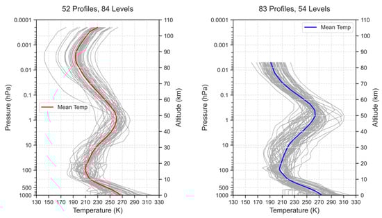
Figure 1.
Temperature distribution in the 52-profile dataset with 84 levels (left) and the standard 83-profile dataset with 54 levels (right). Grey lines represent individual profiles, while red and blue lines represent the mean profiles.
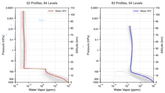
Figure 2.
The same as in Figure 1, but for the results of the water vapor.
2.1.2. SABER Profiles
The Sounding of the Atmosphere using Broadband Emission Radiometry (SABER) instrument, manufactured by Space Dynamics Laboratory, Utah State University, North Logan, Utah, USA, is carried aboard the Thermosphere Ionosphere Mesosphere Energetics and Dynamics (TIMED) satellite, which was funded by the National Aeronautics and Space Administration (NASA). SABER is equipped with 10 channels, covering a spectral range of 1.27–17 μm, enabling global atmospheric detection [21,22]. The TIMED satellite was launched in December 2001, and SABER data have been continuously acquired from 2002 to the present. The observation altitude for SABER Level 2A products ranges from 10 to 200 km, where the effective observations for temperature, pressure, and density profiles are about 10–105 km. Level 2B products can be further extended over 105 km [22]. The SABER product has now been updated to version 2.0 (V2.0).
The SABER V2.0 data primarily includes Level 1B, Level 2A, Level 2B, and Level 2C products. Level 1B products consist of calibrated radiance profiles, providing foundational data for subsequent retrieval. Level 2A routine observation products include vertical profiles of kinetic temperature, pressure, density, and geopotential altitude, as well as emission rates for nitrogen oxide (NO), hydroxyl (-OH), and oxygen (O2), and mixing ratios for ozone (O3), water vapor (H2O), carbon dioxide (CO2), oxygen (O), hydrogen (H) [22,23]. Level 2B data are primarily derived from Level 2A observation parameters through physical models and algorithms, covering temperature and density, CO2 concentration, oxygen and hydrogen atom concentrations, geostationary wind fields, atmospheric cooling rates, and other parameters above 105 km. They are mainly used to study scientific issues such as atmospheric energy balance, chemical reaction kinetics, and upper atmospheric circulation.
Compared to version 1.07 (V1.07), the retrieval algorithm and radiance calibration of the SABER V2.0 dataset are optimized. For example, radiance has been recalibrated to enhance observational accuracy. All observations utilize the retrieval of atomic oxygen concentration, while version V1.07 uses it only during daytime observations (solar zenith angle < 85°). Additionally, V2.0 updated the Whole Atmosphere Community Climate Model (WACCM) to simulate CO2 concentration. It also adjusts reaction rates within the CO2 vibrational temperature model to optimize temperature retrieval under non-local thermodynamic equilibrium (NLTE) conditions. These improvements have been particularly effective in observations of the atmosphere at 75–105 km, significantly reducing systematic errors in temperature retrieval [21,24]. The 2024 SABER V2.0 Level 2A data product used in this study is open access at: http://saber.gats-inc.com/ (accessed on 17 March 2025).
2.1.3. Magnetic Field Profiles
The Zeeman splitting effect is directly related to the applied magnetic field. For simplicity of analysis, the O2 fine-structure simulations in the upper atmosphere are primarily regulated by the Earth’s magnetic field. The International Geomagnetic Reference Field (IGRF) model has been widely used in simulating the microwave upper atmospheric sounding (UAS) channel [14,25]. The IGRF is updated every five years, providing a standardized framework for modeling and predicting the global magnetic field. The 2024 Earth’s magnetic field strength and direction can be derived from the IGRF-13 [26]. In this study, a 3D atmosphere-magnetic coupling dataset is constructed based on the IGRF-13 and the SABER V2.0 Level 2A product. By using this 3D coupling dataset, the 2D geomagnetic field at a fixed altitude (e.g., 60 km) or the magnetic field profile corresponding to a real altitude can be flexibly selected for radiance simulation.
The SABER has a yaw cycle of approximately two months (60 days), causing its observation region alternate between 53°S–83°N and 83°S–53°N every two months [22,24]. Therefore, the 3D coupling dataset constructed in this study exhibits the same yaw cycle characteristics as SABER. Figure 3 displays the global magnetic field profile distribution of the 3D atmosphere-magnetic field coupling dataset for 1 January and 1 August 2024. As shown in Figure 3, the primary observation hemisphere for SABER is the Northern Hemisphere on 1 January, with vertical magnetic field profiles covering latitudes from 53°S to 83°N. By August 1, the primary observation hemisphere shifted to the Southern Hemisphere, with vertical magnetic field profiles covering latitudes from 83°S to 53°N. This figure also indicates that various magnetic field strengths correspond to different altitudes in certain areas, which may affect radiance simulations.
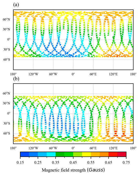
Figure 3.
Global magnetic field profile distribution of the 3D atmosphere-magnetic coupling dataset on (a) 1 January 2024 and (b) 1 August 2024.
2.2. RS-LBL Model
The key to developing a forward RTM for passive microwave sensors is to establish a quantitative relationship between atmospheric states and satellite radiances. The essence is providing an accurate mathematical description of the physical process by which radiation propagates from the Earth’s surface through the atmosphere to the receiver. The simulation accuracy of the RTM depends on the ability of the surface, atmosphere, and sensor to characterize physical processes, as well as the appropriateness of mathematical approximations employed to reduce computational complexity [27]. In this study, O2 absorption lines split into polarized sublines under the influence of an external magnetic field (i.e., the Zeeman effect). This effect significantly reduces the accuracy of RTM simulations at altitudes above 40 km and must be considered.
To fully describe the propagation of radiation in polarized absorbing media, reference [28] defined the power coherence matrix and the brightness temperature (BT) matrix:
where the diagonal elements and represent the brightness temperatures for circularly- or linearly-based polarization. The off-diagonal elements and are used to describe the coherence between horizontal and vertical linear or right-hand and left-hand circular polarizations.
The vector radiative transfer equations for emitting and absorbing media were derived, and the general solution for the BT matrix was also obtained. Ultimately, a radiative transfer equation in the form of a coherence matrix was established that fully expresses polarization information [28]. Based on this theoretical framework, a microwave Line-by-Line model was developed, which can be used to solve the linearly based polarization BT matrix in the upper atmosphere [29]. However, this model neglects the phase term when calculating the microwave oxygen spectrum thermal radiation, which can introduce a simulation bias up to 1.5 K [30]. To address this, reference [30] developed an LBL radiative transfer model incorporating phase terms (RS-LBL (version 1988), also the RS88 model), which has been widely used to train fast RTM coefficients (e.g., Community Radiative Transfer Model, CRTM) [19,25]. The Rosenkranz team has continuously maintained and updated the microwave LBL model at: https://cetemps.aquila.infn.it/mwrnet/lblmrt_ns.html (accessed on 17 March 2025), with the latest version released as the RS-LBL model (version 2024). The primary differences between versions of the RS-LBL model are computational accuracy optimization and updates to absorption gas intensity, broadening parameters, and mixing coefficients based on the latest research [31,32,33,34]. For this study, the most significant update in the RS-LBL model is the improvement to the Zeeman splitting coefficient. The Zeeman splitting coefficient directly influences the frequency shift and intensity of O2 absorption lines. This coefficient is governed by the so-called ‘g-factor’, which is commonly used to quantify the intensity of the interaction between magnetic fields and specific energy levels of oxygen molecules.
Previous microwave LBL models, such as the Millimeter-Wave Propagation Model (MPM) [35], the RS-LBL (version 1988) (RS88) model [30], and ARTS calculations before 2014 [36], all employed Hund’s case (b) basis wavefunctions to determine the Zeeman splitting coefficient. This model is dominated by the electron spin Zeeman effect, neglecting the fine-structure Hamiltonian off-diagonal elements and higher-order Zeeman effects.
where the S is the electronic spin-quantum number. This model is dominated by the electron spin Zeeman effect, neglecting the fine-structure Hamiltonian off-diagonal elements and higher-order Zeeman effects.
In 2019, an updated Zeeman splitting coefficient calculation method was proposed, incorporating higher-order rotational and anisotropic spin Zeeman effects [17]:
where is the diagonalization angle, determined by the ratio of the off-diagonal elements to the diagonal elements in the fine-structure Hamiltonians. For the derivation of , , , and , and also for the calculation results of , , and , please refer to [17]. Theoretically, this improvement can effectively enhance the computational accuracy of the Zeeman effect in low-energy oxygen molecules, thereby improving the inversion of atmospheric temperature and magnetic field profiles, as well as the radiation simulation accuracy of satellite or ground-based instruments.
3. Results
The SSMIS onboard the Defense Meteorology Satellite Program’s Flight 17 (DMSP-F17) observations in 2024 are utilized to investigate factors influencing microwave radiative transfer simulations. Specifically, SSMIS channels 19 and 20 are selected, with peak detection heights of 0.2 hPa and 0.08 hPa, respectively. To achieve accurate comparison with observations, input profiles derived from the SABER V2.0 Level 2A and the IGRF-13 dataset are matched with SSMIS observations based on three strict principles: 1. The latitude and longitude absolute difference between two data points is less than 2°, and the distance between the two points is the smallest of all data pairs. 2. The absolute time difference between observations is less than 1 h. 3. SSMIS channel 19 is matched according to a height of 0.2 ± 0.1 hPa, and channel 20 is matched at 0.08 ± 0.1 hPa. The 1st and 2nd of each month from January to December 2024 are selected for this experiment, totaling 24 days of observation. Building on the foundational research of prior studies [14,17], this study systematically investigates and compares the effects of geomagnetic field dimensions and Zeeman splitting coefficients on the RS-LBL model simulation.
3.1. Impact of Geomagnetic Field Dimensions
To simplify the analysis, only the Earth’s magnetic field is incorporated as the external magnetic field in the radiative transfer simulation. For the 2D Earth’s magnetic field simulation experiments, the northward, eastward, and downward geomagnetic components at an altitude of 60 km are derived from the IGRF-13. The total magnetic field strength (Be) and the cosine of the angle between the magnetic field vector and the electromagnetic wave propagation direction (cos(θ)) are calculated as input for the RS-LBL model. As for the 3D experiment, the Be and cos(θ) profiles derived from the 3D coupling dataset mentioned in Section 2.1.3 are employed. To validate the effectiveness of this 3D coupling dataset, the vertical average of temperature and geomagnetic field profiles is first calculated over a 24-day experimental cycle. For the cos(θ) calculation, the zenith angle and azimuth angle are assumed to be 53.1° and 0°, respectively, to eliminate interference from the observational angle. Furthermore, 100 independent temperature and geomagnetic field profile sets are randomly selected from the 24-day experimental data as supplementary validation samples.
Figure 4 shows the vertical distribution of Temperature, Be, and cos(θ) average calculated based on the 3D coupling dataset, along with the corresponding 100 random profiles. As seen in Figure 4, atmospheric temperature increases with altitude of 100–1 hPa (16–48 km), which is consistent with the temperature distribution in the stratosphere. At altitudes between 1 and 0.01 hPa (48–80 km), atmospheric temperature decreases with altitude, corresponding to the temperature distribution of the mesosphere. When the altitude exceeds 0.01 hPa (80 km), the mean temperature profile from SABER shows no significant trend with altitude. This may be because the SABER dataset used in this experiment includes different seasons, causing the mean profile to be averaged out. Comparing the SABER temperature profile in Figure 4 with the ECMWF model profile (Figure 1), the distribution of the two mean temperature profiles is similar between 100 and 0.01 hPa. Both exhibit a peak value of approximately 260 K near 1 hPa. However, each SABER temperature profile (grey lines) exhibits significant fluctuations above 0.01 hPa, while the ECMWF model profile temperatures all decrease with altitude. The vertical distribution of the total magnetic field strength (Figure 4b) indicates that it gradually decreases with altitude, but the variation is smaller than that of temperature. As for cos(θ) (Figure 4c), its pattern is difficult to assess visually, and quantitative statistics are needed for further analysis.
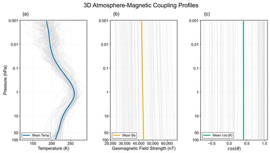
Figure 4.
Distribution of 3D atmosphere-magnetic coupling dataset: (a) temperature, (b) total magnetic field strength (Be), and (c) cosine of the angle between the magnetic field vector and the electromagnetic wave propagation direction (cos(θ)). The blue, yellow, and green lines represent the mean temperature, Be, and cos(θ) for the 24 days from the 1st to the 2nd of each month from January to December 2024, respectively. Grey lines represent 100 individual profiles randomly selected from the entire experimental dataset.
To compare the effects of 2D and 3D geomagnetic parameters on microwave radiative transfer simulations, this study statistically analyzed the difference between observed and simulated BT (O-B) under both geomagnetic inputs. Generally, the geomagnetic field strength exhibits significant latitude dependence, meaning that it is typically stronger at high latitudes and relatively weaker at low latitudes, such as at the equator. The global latitudinal distribution of O-B for SSMIS channels 19 and 20 is presented in Figure 5. The statistics covered latitudes from 90°S to 90°N, with averages calculated every 10° intervals. As seen in Figure 5, most of the SSMIS channels 19 and 20 O-B are improved across all global latitudes when 3D geomagnetic profiles are used as input (orange curve). This demonstrates that incorporating 3D geomagnetic field parameters can universally enhance the microwave RTM simulations.
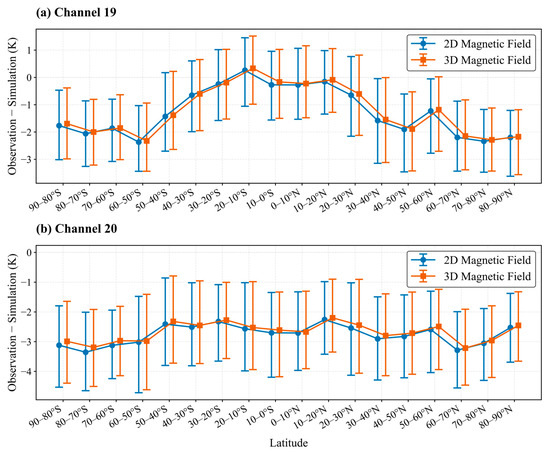
Figure 5.
Distribution of DMSP-F17 SSMIS (a) channel 19 and (b) channel 20 observation and simulation biases (O-B) with global latitude (statistics by every 10°). Blue represents simulation results using the two-dimensional (2D) Earth’s magnetic field as input, while orange indicates simulation results using the three-dimensional (3D) Earth’s magnetic field.
To further validate the physical mechanisms underlying this enhancement, a quantitative calculation of the vertical attenuation of Be is performed using all 24-day profiles from the 3D atmosphere-magnetic coupling dataset. The average attenuation of the total geomagnetic field strength from 50 hPa to 0.001 hPa altitude is approximately 1290.5 nT, with a relative attenuation rate of 2.98%. The Be average and relative difference between two locations (55°S, 30°W and 55°S, 120°E) at approximately 60 km altitude is also calculated based on the horizontal distribution. Results indicate that at the same latitude, the average difference of total geomagnetic field strength between the two regions is approximately 37,447.3 nT. The geomagnetic strength near 120°E is 141.30% higher than that at 30°W, which will introduce an approximately 10 K simulation difference.
The O-B for SSMIS channels 19 and 20 are statistically analyzed to validate the impact of the 2D and 3D geomagnetic field on the brightness temperature simulations. Figure 6 shows the O-B probability density functions (PDF) for SSMIS channels 19 and 20 onboard the DMSP-F17 satellite during the 24-day experiment in 2024. The PDF of O-B based on 2D and 3D geomagnetic fields are represented by blue and orange bars, respectively. From Figure 6, the probability of O-B being close to 0 K is higher when using the 3D geomagnetic field as input. Further statistics are calculated for the mean, median, root mean square error (RMSE), and mean absolute error (MAE) of the two experimental O-Bs, as shown in Table 1. The change rate (Unit: %) shown in Table 1 is used to quantify the improvement of the O-B based on the 3D geomagnetic field relative to the 2D one. If the change rate is negative, it indicates that the simulation bias of the 3D experiment is lower than that of the 2D experiment. The larger the absolute value of the change rate, the more pronounced the simulation departure between the two experiments. According to Table 1, the absolute values of the mean and median O-B for SSMIS channels 19 and 20 using 3D geomagnetic field parameters as input are both smaller than those for 2D. Channel 20 has a higher detection altitude, thereby achieving a more significant improvement in simulation compared to channel 19. However, the change rates for channels 19 and 20 are both negative, with values exceeding 3.5. Compared to the average magnetic field attenuation rate of 2.98%, the 3.5% improvement in average simulated brightness temperature is reasonable. Additionally, after applying the 3D geomagnetic field parameters, both the RMSE and MAE for SSMIS channels 19 and 20 appear improved. Although the vertical variation of the Earth’s magnetic field is far smaller than its horizontal variation, experimental results indicate that the RS-LBL model can still capture this subtle vertical attenuation signal when simulating SSMIS channels 19 and 20.
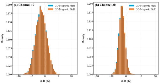
Figure 6.
The O-B probability density functions (PDF) of DMSP-F17 SSMIS (a) channel 19 and (b) 20. The blue and orange represent the PDF derived from the 2D and 3D geomagnetic field parameters, respectively.

Table 1.
O-B statistics for SSMIS channels 19 and 20 based on 2D and 3D geomagnetic fields.
3.2. Effect of Zeeman Splitting Coefficients
3.2.1. RS-LBL Model Simulation Difference
Microwave radiometers and sounders for middle and upper atmosphere detection typically select channels near the center frequencies of oxygen absorption lines, including 1− (118.7503 GHz), 11− (57.6125 GHz), 13− (56.9682 GHz), 7+ (60.4348 GHz), 9+ (61.1506 GHz), 15+ (62.9980 GHz), and 17+ (63.5685 GHz) lines, such as those used by the Microwave Limb Sounder (MLS) [37], Advanced Microwave Sounding Unit A (AMSU-A) channels 11–14 [9], and SSMIS channels 19–24 [38]. In this section, the Hund’s case (b) and reference [17] implementation of the RS-LBL model, adopted in the 1988 and 2024 versions (V_1988 and V_2024), respectively, are employed to calculate the Stokes vector under the following conditions: total magnetic field strength Be and angle between the magnetic field vector and the electromagnetic wave propagation direction (θ) are set to fixed values of 0.5 Gauss and 135°, respectively, and the O2 absorption lines center frequency are shifted by ±4 MHz in steps of 0.1 MHz. Figure 7 shows the simulation differences between the V_1988 and V_2024 of the RS-LBL model for specific O2 absorption lines.
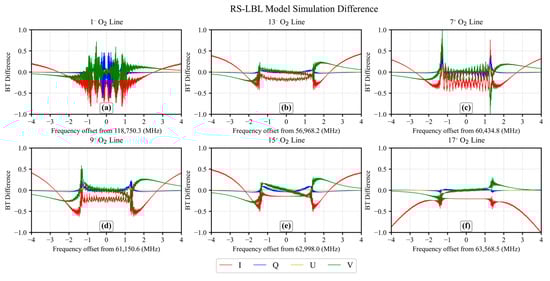
Figure 7.
Stokes vector simulation differences between the version 1988 (V_1988) and version 2024 (V_2024) of the RS-LBL model for Be = 0.5 Gauss and θ = 135° at frequency shift of ±4 MHz in step of 0.1 MHz from: (a) 1− (118.7503 GHz); (b) 13− (56.9682 GHz); (c) 7+ (60.4348 GHz); (d) 9+ (61.1506 GHz); (e) 15+ (62.9980 GHz); and (f) 17+ (63.5685 GHz) line. The red line represents I, the blue represents Q, the yellow represents U, and the green represents V.
As shown in Figure 7, the simulation differences of Stokes Q, U, and V components at the line center are relatively small. The difference oscillatory increases with frequency offset and reaches a peak at approximately 1.4 MHz, except for the 1− line. This is because the correction to the Zeeman splitting coefficient alters the spacing between magnetic energy levels, affecting the absorption cross-section at different frequencies. In the wings (at frequency offset of about 1.4 MHz), the cross-section difference is more pronounced because absorption remains unsaturated. When absorption saturation occurs, the absorption intensity difference between the RS-LBL models will be compressed, such as at the line center [17]. It is noteworthy that the simulated difference of 1− line is unique, showing no discernible trend with frequency shift. It can be confirmed that within the ±2 MHz frequency shift, the 1− line simulation difference of I, Q, and V components all exceed 0.5 K. Overall, the simulation differences for the 1− and 7+ lines are more pronounced than other lines, consistent with the theory proposed by reference [17].
Considering the limitations of simulating the Zeeman splitting effect under a single Be and θ, a broader range of geomagnetic field parameters is required. Therefore, Be and θ are upgraded from constants to ranges constrained by real atmospheric conditions and are used as inputs for the RS-LBL model simulation. Specifically, the frequency is set to a fixed value, while the Be and θ are systematically varied: Be from 0.2 Gauss to 0.7 Gauss in steps of 0.01 Gauss, and θ from 0° to 180° in steps of 1°. At the 50–70 GHz band, the 7+ line has stronger absorption intensity and is widely used in microwave remote sensing, making it a suitable choice for this experiment. The 1− line possesses a unique frequency position in the O2 absorption spectrum and is also selected for simulation. According to Figure 7, the 7+ and 1− lines exhibit significant simulation differences at frequency offsets of approximately 1.4 MHz and −0.5 MHz, respectively. Therefore, two fixed frequencies are selected for this experiment: 60.4362 GHz (7+ line center frequency offset of 1.4 MHz) and 118.7498 GHz (1− line center frequency offset of −0.5 MHz).
Figure 8 and Figure 9 illustrate the RS-LBL model simulation differences of the Stokes parameters I, Q, U, and V under fixed frequencies and varying magnetic fields. Typically, I represents the total radiance intensity, Q denotes the difference between vertical and horizontal linear polarization, U indicates the difference between ±45° linear polarization, and V signifies the difference between left- and right-hand circular polarization [39]. As seen in Figure 8, the simulated difference of total intensity I exhibits significant fluctuations with respect to Be and θ. This is because I represents the superposition of all magnetic energy level transition signals, reflecting the global characteristic of the Zeeman splitting effect. In contrast, the circular polarization component V exhibits alternative positive and negative variations with θ at a fixed magnetic field strength. Its amplitude is comparable to that of I, but approaches zero near θ = 90°. This phenomenon indicates that the simulation differences between left- and right-hand circular polarizations follow an antisymmetric distribution with θ. When the magnetic field vector is perpendicular to the electromagnetic wave propagation direction, these simulation differences cancel each other out. Overall, the simulated differences of I, Q, and V are greater than that of U. This may be due to the azimuthal symmetry of the angle between the magnetic field vector and the electromagnetic wave propagation direction, leading to significant signal suppression of the U component. For the 1− line (Figure 9), the simulated difference of the I component is relatively weak, generally around 0.15 K. Beyond the influence of frequency selection, this subtle difference is also related to the unique energy level transition structure of the 1− line. According to reference [17], the Zeeman ‘g-factor’ for the low-energy level of the 1− line does not couple with the magnetic field. Therefore, the simulation difference is only attributable to higher-order Zeeman effect corrections at higher energy levels. Similar to the 7+ line, the U component of the 1− line still exhibits minimal simulation differences. Meanwhile, the difference of the V component, which represents the circular polarization, alternates between positive and negative with θ at a fixed magnetic field strength.
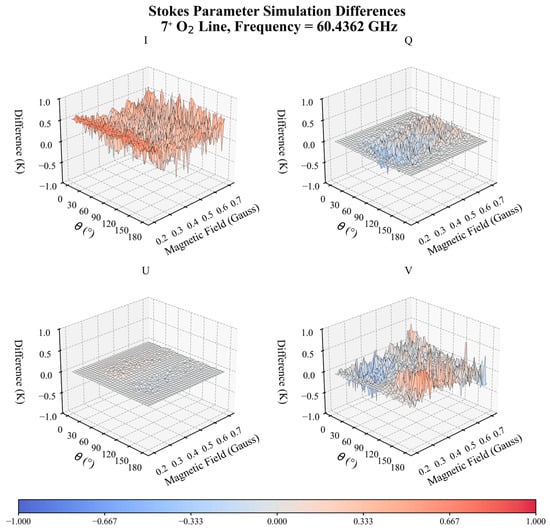
Figure 8.
Version 1988 and version 2024 of the RS-LBL model Stokes vector (I, Q, U, and V) simulation difference at 60.4362 GHz (7+ line frequency shift 1.4 MHz) on total magnetic field strength Be ranges from 0.2–0.7 Gauss in steps of 0.1 Gauss; the angle between the magnetic field vector and the electromagnetic wave propagation direction θ ranges from 0° to 180° in steps of 1°.
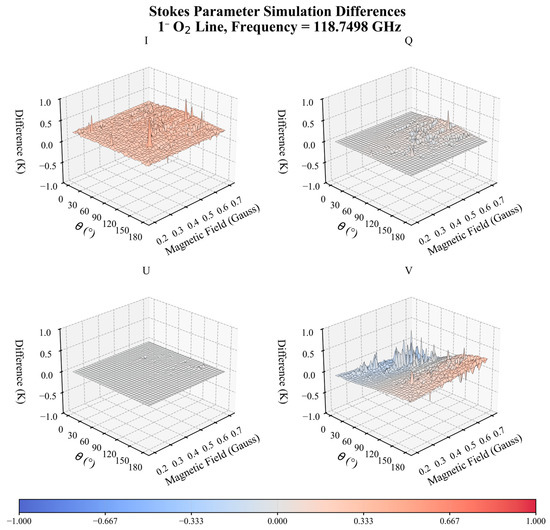
Figure 9.
The same as in Figure 8, but for the results of 118.7498 GHz (1− line frequency shift −0.5 MHz).
3.2.2. Observation Validation
Although the Zeeman splitting correction has a negligible effect on the simulation of the 1− line (the energy level transition with angular momentum 0), it still significantly impacts the 7+ line with intermediate . The authors of reference [17] have theoretically demonstrated the superiority of this improvement. However, whether the updated Zeeman splitting coefficient can improve the simulation accuracy of the RS-LBL model still requires validation through real observations. The detection frequency of SSMIS channel 20 is based on the 7+ and 9+ O2 absorption lines [40], enabling the assessment of Zeeman splitting coefficient corrections on real observations and applications. Therefore, the atmospheric and geomagnetic field parameters derived from SABER V2.0 and IGRF-13, respectively, are used as input profiles for the V_1988 and V_2024 of the RS-LBL model. Observations from the 1st to the 2nd of each month in 2024 (totaling 24 days) of DMSP-F17 SSMIS channel 20 are used to validate the RS-LBL model simulation differences. The O-B is statistically averaged for each 10° latitude band, as shown in Figure 10.
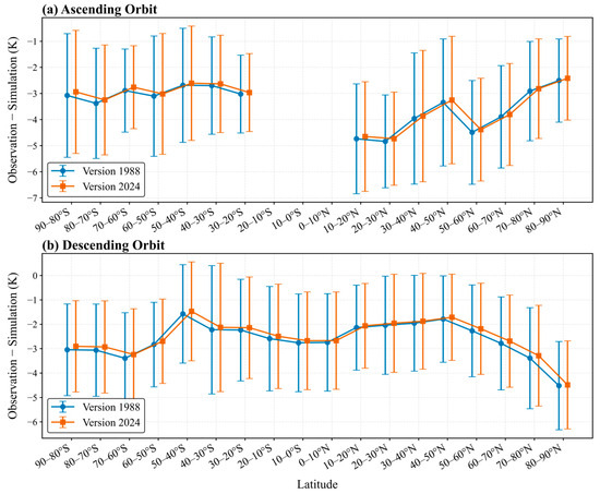
Figure 10.
Global latitude O-B distribution statistics of (a) ascending orbit and (b) descending orbit observations from DMAP-F17 SSMIS channel 20 between RS-LBL (version 1988) and RS-LBL (version 2024), respectively. Blue represents the results of the V_1988 RS-LBL, while orange indicates the V_2024.
In Figure 10, the RS-LBL model O-B from V_2024 shows overall improvement compared to V_1988. Despite the SSMIS Channel 20 ascending orbit exhibiting observation gaps at the equator, the V_2024 model demonstrates superior simulation capability at middle and high latitudes, particularly in polar areas. Overall, the simulation differences between the two models are most pronounced south of 60°N and north of 50°S. This is primarily because magnetic field strength is generally greater in middle and high latitudes than at the equator, and the Zeeman effect is extremely sensitive to variations in magnetic field strength.
To quantitatively evaluate the improvement in radiative transfer simulation by the updated Zeeman splitting coefficient, statistical analysis of O-B from the two RS-LBL models (V_1988 and V_2024) is conducted over 24 days. The mean bias, MAE, and RMSE are evaluated in this study, with results shown in Figure 11. As can be seen in Figure 11, the MAE, RMSE, and mean bias of V_2024 all improved at both ascending and descending orbits compared to V_1988. Specifically, MAE and RMSE decreased from 3.46 K to 3.37 K and from 3.97 K to 3.89 K, respectively, for ascending orbits. For descending orbits, MAE decreased from 2.69 K to 2.62 K and RMSE decreased from 3.20 K to 3.12 K. As for mean O-B, the absolute values of ascending orbits are generally greater than those of descending orbits. This may be related to the observation gap in the ascending orbit at low latitude. However, both the ascending and descending orbits achieved a mean bias improvement of 0.1 K. Overall, V_2024 achieved a 2.8% MAE improvement at the descending orbit, slightly exceeding the 2.6% for the ascending orbit. For RMSE, the improvement on the descending orbit reached 2.4%, also higher than the 2.1% for ascending orbits.
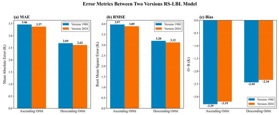
Figure 11.
DMAP-F17 SSMIS channel 20 observation and simulation bias of RS-LBL model V_1988 (blue) and V_2024 (orange) statistics results: (a) mean absolute error (MAE), (b) root mean square error (RMSE), and (c) mean O-B. The bold numbers in the figure represent specific statistical values (unit: K).
In summary, the V_2024 RS-LBL model achieved positive optimization across MAE, RMSE, and mean O-B. These results fully validate the systematic improvement in updating Zeeman splitting coefficients and oxygen absorption parameters. According to Figure 7, the simulation difference in total radiation intensity I between the two RS-LBL models for the 7+ and 9+ lines with a frequency shift of less than 1 MHz is approximately 0.1–0.2 K, with smaller departures near the line centers. The SSMIS channel 20 bandwidth is 1.35 MHz, covering this frequency shift range. Therefore, the simulated improvement of 0.1 K validated through real observation is justified.
4. Discussion
According to the analysis in Section 3.1, even a minimal vertical variation in the total magnetic field strength can affect the simulations of the SSMIS UAS channel. However, the magnetic field environment in the real upper atmosphere is far from being as uniform and stable as in the description by the IGRF model. In addition to Earth’s magnetic field, external magnetic fields such as the solar wind and interplanetary magnetic field may also introduce additional disturbances to observations and simulations. Particularly during geomagnetic storms, significant magnetic field fluctuations occur in localized regions such as the polar areas. To investigate the influence of Be and θ on microwave radiation simulations, atmospheric profiles with 84 levels derived from the ECMWF model (Figure 1 and Figure 2) are used as input for the V_2024 RS-LBL model. The dependence of O2 absorption line simulations on Be and θ is systematically discussed.
4.1. Magnetic Field Strength
To evaluate the effect of the Be on the O2 absorption line simulated brightness temperature, cos(θ) is fixed at 0.7. Simulations are conducted within the range of the real Earth’s magnetic field strength, specifically from 0.2 Gauss to 0.7 Gauss in increments of 0.01 Gauss. Figure 12 shows the simulated BT distributions for the right- and left-hand circular, vertical, and horizontal linear polarizations. The simulated frequency shift varies from the 7+ line center toward 0 MHz to 5 MHz in steps of 1 MHz. As shown in Figure 12, the 7+ line exhibits a high-temperature region (260–270 K) across the entire magnetic field strength within the 2–3 MHz frequency offset, with relatively uniform distribution. Based on the temperature distribution in Figure 1 and Figure 4, this high-temperature region largely corresponds to the 1 hPa level. The BT distributions corresponding to different Be values tend to converge when the frequency shift exceeds 3 MHz. This indicates the simulated altitude decrease with a high frequency shift, and the effects of Be and polarization state on BT are significantly weakened or even rendered ineffective. In contrast, BT exhibits significant dependence on Be near the line center, where frequency shifts are less than 2 MHz, with distinct differences in polarization states. Specifically, BT for right-hand circular polarization (Figure 12a) exhibits a relatively gradual variation with magnetic field strength, indicating weak dependence of simulations on Be. While the left-hand circular polarization (Figure 12b) appears to have dense contour lines when Be is around 0.35–0.55 Gauss, accompanied by distinct low-temperature ‘depressions’ (about 210 K). This indicates an exceptionally sensitive response of the simulated brightness temperature to magnetic field strength. The BT distributions for vertical (Figure 12c) and horizontal (Figure 12d) linear polarization exhibit similar patterns, except that vertical polarization shows a more pronounced low signal within the Be at 0.35–0.55 Gauss. From the perspective of a single Be cross-section, the brightness temperature increases with frequency shift within a frequency shift of 4 MHz, particularly when Be is less than 0.35 Gauss. According to Figure 1, the simulated heights of the 7+ line center and its 1 MHz frequency shift reach 75 km and 55 km, respectively, when the magnetic field strength is low. The same analysis is also appropriate to complex BT at middle or high magnetic field strengths, such as the left circular polarization shown in Figure 12b. Additionally, when the frequency offset is opposite of the O2 line center, the simulations for right- and left-hand circular polarization swap at the same magnetic conditions, while linear polarization remains unchanged. This symmetry aligns with the description of frequency symmetry near the line center in Theorem 3 proposed by reference [16].
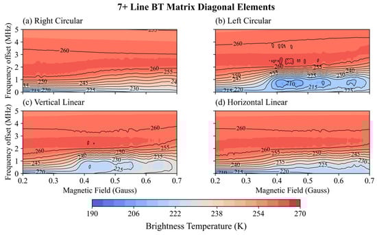
Figure 12.
7+ line center frequency shift from 0–5 MHz (step of 1 MHz), simulated brightness temperature distribution with Be from 0.2 to 0.7 Gauss in steps of 0.01 Gauss for (a) right-hand circular polarization; (b) left-hand circular polarization; (c) vertical linear polarization; and (d) horizontal linear polarization.
Figure 13 displays the simulations for the 1− line. The horizontal axis represents magnetic field strength from 0.2 Gauss to 0.7 Gauss in steps of 0.01 Gauss, while the vertical axis shows the frequency offset from the O2 line center (0–5 MHz increase with 1 MHz). As shown in Figure 13, the isotherms for all four polarizations are nearly horizontal when the frequency shift exceeds 3 MHz, indicating that the effect of Be on simulations is significantly weakened. However, the simulated BTs are extremely sensitive to Be near the line center, especially for left-hand circular and vertical linear polarization. Specifically, extensive low temperatures appear when the Be is larger than 0.5 Gauss. It is noteworthy that the low-temperature area of vertical linear polarization (220–240 K in Figure 13c) is approximately 20 K higher than that of the left-hand circular polarization (204–222 K in Figure 13b). Meanwhile, simulated brightness temperature decreases as the magnetic field strength increases. These phenomena directly reflect how the detection altitude of the 1− line varies with magnetic field strength. Right-hand circular (Figure 13a) and horizontal linear (Figure 13d) polarization have lower dependence on Be but are highly sensitive to frequency offset.
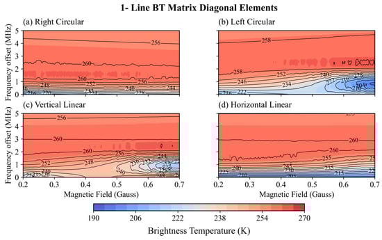
Figure 13.
The same as in Figure 12, but for the results of the 1− line.
In summary, left-hand circular and vertical linear polarization simulations are more sensitive to magnetic field strength, particularly when larger than 0.5 Gauss. However, the right-hand circular and horizontal linear polarizations are more stable, indicating that the physical mechanisms of different polarizations have fundamental differences. However, the above property is only suitable for this experiment, since the simulation also depends on frequency shift, as described in Theorem 3 of reference [16]. From this experiment, the 1− line exhibits greater sensitivity to strong magnetic fields (0.5–0.7 Gauss), while the 7+ line is more sensitive to the moderate Be (0.35–0.55 Gauss). These two lines can be combined for plasma environment diagnostics across different magnetic field strengths, such as distinct eruption areas of solar flares.
4.2. Angular Dependence
Based on the above analysis, the magnetic field strength Be is fixed at 0.45 Gauss in this experiment. The brightness temperature near the 7+ and 1− line center within the θ range from 0° to 180° in steps of 1° (cos(θ) from 1 to −1) is simulated. Figure 14 displays the simulated BT distribution of the 7+ line center frequency shift of 0–5 MHz (step of 1 MHz) for four polarizations. The simulated brightness temperature of θ seems more regular compared to the magnetic field strength. From Figure 14a, the blue low temperature for right-hand circular polarization is primarily concentrated when the frequency offset is less than 1 MHz and cos(θ) < 0 (i.e., 90° < θ < 180°). A peak temperature of 270 K occurs when the 7+ line frequency shift is about 2–3 MHz, similar to that shown in Figure 12a. The simulated BT of the left-hand circular polarization (Figure 14b) exhibits chiral symmetry with respect to the right-hand. For vertical linear polarization (Figure 14c), the low temperature occurs at frequency shifts within 1 MHz and θ between 30° and 150° (), with the lowest brightness temperature appearing near (i.e., θ = 90°). In contrast, the isotherms of the horizontal linear polarization (Figure 14d) simulations are relatively sparse and uniform when the 7+ line frequency shift is above 1 MHz, meaning a weaker dependence on θ.
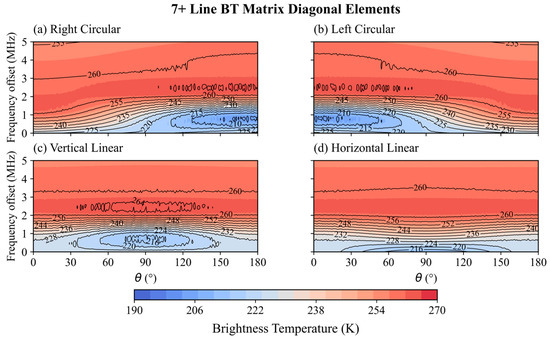
Figure 14.
7+ line center frequency shift from 0 to 5 MHz (step of 1 MHz) simulated brightness temperature distribution with θ from 0 to 180° (step of 1°) for (a) right-hand circular polarization; (b) left-hand circular polarization; (c) vertical linear polarization; and (d) horizontal linear polarization.
The simulated BT for the 1− line is shown in Figure 15, which exhibits a distinct distribution pattern compared to the 7+ line. Except for the horizontal linear polarization simulations, the 1− line has no significant low-temperature area, and the BT is generally higher than the 7+ line when the frequency shift is less than 1 MHz. The layered structure of linearly polarized simulations is clear, and the brightness temperatures increase with frequency shift. When the 1− line frequency shift is 1–2 MHz, the simulated brightness temperature for vertical polarization is more sensitive to frequency compared to θ, whereas horizontal polarization exhibits the opposite behavior. For both the 7+ and 1− line, the linear polarization brightness temperatures are symmetric about cos(θ) = 0 near the line center. This property can be explained using Theorem 1 from reference [16].
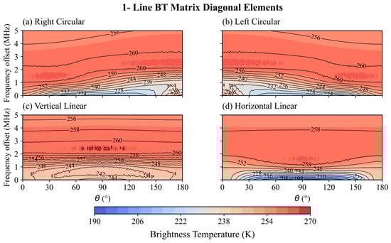
Figure 15.
The same as in Figure 14, but for the results of the 1− line.
5. Conclusions
In this study, the key influencing factors in microwave radiation simulations in the upper atmosphere are investigated. The systematic analysis primarily focuses on the geomagnetic field and the Zeeman effect. A three-dimensional (3D) atmosphere–magnetic coupling dataset is constructed based on the Sounding of the Atmosphere using Broadband Emission Radiometry (SABER) version 2.0 Level 2A atmospheric profiles and the thirteenth generation International Geomagnetic Reference Field (IGRF-13) model. This dataset is then used as input for the microwave radiative transfer model (RTM) developed by Rosenkranz and Staelin (RS-LBL). Observations from the Special Sensor Microwave Imager/Sounder (SSMIS) channels 19 and 20 are used to quantitatively compare the effects of employing two-dimensional (2D) and 3D geomagnetic fields on simulations. Furthermore, the impact of the updated Zeeman splitting coefficient on the simulation of the oxygen (O2) absorption line is also evaluated. The observation and simulation biases (O-B) are statistically and quantitatively analyzed with the global latitude band. In Section 4, atmospheric profiles with 84 levels are used as input for the version 2024 (V_2024) RS-LBL model to investigate the dependence of O2 absorption line simulations on total magnetic field strength (Be) and the angle between the magnetic field vector and the electromagnetic wave propagation direction (θ).
To analyze the impact of geomagnetic field dimensions on simulations, quantitative statistics are conducted on the global horizontal and vertical distribution characteristics of Be. The average variation rate of geomagnetic field strength near 55°S, 30°W to 55°S, 120°E is approximately 141.3%, while the vertical variation rate between 50 and 0.001 hPa is only 2.98%. Using 3D magnetic field parameters as the input improves the O-B for SSMIS channels 19 and 20 by approximately 3.67% and 3.52%, respectively. The results indicate that the RS-LBL model can capture subtle vertical variations in the geomagnetic field from the 3D coupling dataset. Since the vertical variation of the Earth’s magnetic field is not significant, models using IGRF as input can still employ a 2D geomagnetic field to simplify calculations. However, disturbances caused by strong external magnetic fields, such as geomagnetic storms, still need to be considered. The V_2024 RS-LBL model diminishes simulation errors of the low-energy level O2 line by incorporating molecular self-spin interactions and higher-order Zeeman effects. The mean absolute error (MAE) and root mean square error (RMSE) of SSMIS channel 20 are reduced by approximately 2.7% and 2.25%, respectively. Experimental results on the dependence of O2 absorption lines on magnetic field strength indicate that the 7+ line within a frequency shift of 2 MHz is sensitive to moderate Be (0.35–0.55 Gauss). Within this range, pronounced low-temperature depressions appear in both left-hand circular and vertical linear polarization. The 1− line is more sensitive to strong magnetic fields (0.5–0.7 Gauss), and a complex brightness temperature (BT) structure displays when the frequency shift is less than 1 MHz. This is because the O2 absorption lines near the 118.75 GHz line and the 50–70 GHz lines exhibit different transition characteristics.
Via comparisons with the SSMIS observations, this study demonstrates that optimizing the geomagnetic field and the Zeeman effect can improve upper atmospheric microwave RTM simulation accuracy. This provides critical technical support for the application of satellite observations in the numerical weather prediction (NWP) system, also expanding the potential of O2 absorption lines in space weather detection. However, several shortcomings remain in this study: First, the IGRF-13 model can only characterize large-scale geomagnetic field parameters, which cannot capture local magnetic disturbances. Second, this experiment assumes the content of water vapor and ozone content, and that the mixing ratio of oxygen is constant, neglecting the impact of their vertical distribution on simulations. Third, this study only discusses the 7+ and 1− lines, and only two channels of the SSMIS are used for evaluation. Oxygen absorption lines at lower energy levels than the 7+ line, and additional observations are required for further study. Additionally, the results of this study indicate that channels 19 and 20 of the SSMIS exhibit a systematic bias of approximately 2–3 K between observations and simulations. The causes of this phenomenon are multifaceted: 1. Potential observational biases in the SSMIS upper atmospheric sounding (UAS) channel; 2. Modeling errors inherent to the RS-LBL model itself; 3. Existing bias between atmospheric temperature and geomagnetic field profiles (derived from the SABER and IGRF datasets) and the real atmosphere; and 4. Certain reasonable assumptions being made during the experiment. However, this stable systematic bias can be reasonably eliminated in actual applications.
As an extension of this study, observed geomagnetic parameters can be merged to construct a real-time 3D geomagnetic coupling dataset. This can be used to investigate space weather events on microwave RTM simulations. The fast RTM optimized in the same way as the RS-LBL model can be employed in NWP systems to evaluate its effectiveness for upper-level atmospheric temperature forecast accuracy. Since this study only considered the effects of magnetic fields and Zeeman splitting coefficients on simulations, other influencing factors remain to be investigated. Furthermore, due to the limitations of upper atmospheric microwave observations and radiative transfer models, all existing models and observations should be fully utilized to conduct further research. Based on the sensitivity of oxygen lines to magnetic fields, a new generation of microwave detection channel parameters for the middle and upper atmosphere can be designed. This would also provide additional observations in support of studying upper atmospheric characteristics.
Author Contributions
Conceptualization, C.D. and F.W.; methodology, C.D. and F.W.; software, C.D. and E.T.; validation, C.D., F.W. and E.T.; formal analysis, C.D.; investigation, C.D.; resources, F.W.; data curation, C.D.; writing—original draft preparation, C.D.; writing—review and editing, F.W. and E.T.; visualization, C.D.; supervision, F.W.; project administration, F.W.; funding acquisition, F.W. All authors have read and agreed to the published version of the manuscript.
Funding
This research is supported by the National Natural Science Foundation of China grant (U2242211 and U2542208).
Data Availability Statement
The SABER V2.0 Level 2A data can be downloaded from the website: https://data.gats-inc.com/saber/ (accessed on 17 March 2025). Further inquiries can be directed to the corresponding author.
Acknowledgments
We sincerely thank the reviewers and the editors for their insightful comments.
Conflicts of Interest
The authors declare no conflicts of interest.
Abbreviations
The following abbreviations are used in this manuscript:
| NWP | Numerical Weather Prediction |
| MLS | Microwave Limb Sounder |
| SABER | Sounding of the Atmosphere using Broadband Emission Radiometry |
| DMSP | Defense Meteorology Satellite Program |
| SSMIS | Special Sensor Microwave Imager/Sounder |
| AMSU-A | Advanced Microwave Sounding Unit A |
| MAS | Millimeter-wave Atmospheric Sounder |
| TIMED | Thermosphere Ionosphere Mesosphere Energetics and Dynamics |
| NASA | National Aeronautics and Space Administration |
| ECMWF | European Centre for Medium-Range Weather Forecasts |
| UAS | Upper Atmospheric Sounding |
| IGRF | International Geomagnetic Reference Field |
| HALOE | Halogen Occultation Experiment |
| BT | Brightness Temperature |
| O2 | Oxygen |
| 3D | three-dimensional |
| 2D | two-dimensional |
| NLTE | non-local thermodynamic equilibrium |
| O-B | observation minus simulation |
| RMSE | root mean square error |
| MAE | mean absolute error |
| WACCM | Whole Atmosphere Community Climate Model |
| RTM | radiative transfer model |
| RS-LBL | Rosenkranz and Staelin’s microwave Line-by-Line |
| MPM | Millimeter-Wave Propagation Model |
| ZPM | Zeeman Propagation Model |
| ARTS | Atmospheric Radiative Transfer Simulator |
| RTTOV | Radiative Transfer for the TIROS Operational Vertical Sounder |
| CRTM | Community Radiative Transfer Model |
References
- Zhao, X.R.; Sheng, Z.; Shi, H.Q.; Weng, L.B.; He, Y. Middle Atmosphere Temperature Changes Derived from SABER Observations during 2002–2020. J. Clim. 2021, 34, 7995–8012. [Google Scholar] [CrossRef]
- Liu, L.; Bliankinshtein, N.; Huang, Y.; Gyakum, J.R.; Gabriel, P.M.; Xu, S.; Wolde, M. Comparative Experimental Validation of Microwave Hyperspectral Atmospheric Soundings in Clear-Sky Conditions. Atmos. Meas. Tech. 2025, 18, 471–485. [Google Scholar] [CrossRef]
- Eckermann, S.D.; Ma, J.; Hoppel, K.W.; Kuhl, D.D.; Allen, D.R.; Doyle, J.A.; Viner, K.C.; Ruston, B.C.; Baker, N.L.; Swadley, S.D.; et al. High-Altitude (0–100 km) Global Atmospheric Reanalysis System: Description and Application to the 2014 Austral Winter of the Deep Propagating Gravity Wave Experiment (DEEPWAVE). Mon. Weather Rev. 2018, 146, 2639–2666. [Google Scholar] [CrossRef]
- Eckermann, S.D.; Hoppel, K.W.; Coy, L.; McCormack, J.P.; Siskind, D.E.; Nielsen, K.; Kochenash, A.; Stevens, M.H.; Englert, C.R.; Singer, W.; et al. High-Altitude Data Assimilation System Experiments for the Northern Summer Mesosphere Season of 2007. J. Atmos. Sol.-Terr. Phys. 2009, 71, 531–551. [Google Scholar] [CrossRef]
- Hoppel, K.W.; Baker, N.L.; Coy, L.; Eckermann, S.D.; McCormack, J.P.; Nedoluha, G.E.; Siskind, E. Assimilation of Stratospheric and Mesospheric Temperatures from MLS and SABER into a Global NWP Model. Atmos. Chem. Phys. 2008, 8, 6103–6116. [Google Scholar] [CrossRef]
- Hoppel, K.W.; Eckermann, S.D.; Coy, L.; Nedoluha, G.E.; Allen, D.R.; Swadley, S.D.; Baker, N.L. Evaluation of SSMIS Upper Atmosphere Sounding Channels for High-Altitude Data Assimilation. Mon. Weather Rev. 2013, 141, 3314–3330. [Google Scholar] [CrossRef]
- Maurer, T.; Ruston, B.; Swadley, S.; Booton, A. Assimilation Impacts of SSMIS Upper Atmosphere Soundings with Improved Orbital Bias Predictors in NAVGEM. In Proceedings of the 20th International TOVS Study Conference (ITSC-20); International TOVS Working Group: Lake Geneva, WI, USA, 2015. [Google Scholar]
- Nezlin, Y.; Rochon, Y.J.; Polavarapu, S. Impact of Tropospheric and Stratospheric Data Assimilation on Mesospheric Prediction. Tellus A 2009, 61, 154–159. [Google Scholar] [CrossRef]
- Dong, C.; Hu, H.; Weng, F. Optimal Assimilation of Microwave Upper-Level Sounding Data in CMA-GFS. Adv. Atmos. Sci. 2024, 41, 2043–2060. [Google Scholar] [CrossRef]
- Meeks, M.L.; Lilley, A.E. The Microwave Spectrum of Oxygen in the Earth’s Atmosphere. J. Geophys. Res. 1963, 68, 1683–1703. [Google Scholar] [CrossRef]
- Hartmann, G.K.; Degenhardt, W.; Richards, M.L.; Liebe, H.J.; Hufford, G.A.; Cotton, M.G.; Bevilacqua, R.M.; Olivero, J.J.; Kämpfer, N.; Langen, J. Zeeman Splitting of the 61 Gigahertz Oxygen (O2) Line in the Mesosphere. Geophys. Res. Lett. 1996, 23, 2329–2332. [Google Scholar] [CrossRef]
- Zeeman, P. XXXII. On the Influence of Magnetism on the Nature of the Light Emitted by a Substance. Lond. Edinb. Dublin Philos. Mag. J. Sci. 1897, 43, 226–239. [Google Scholar] [CrossRef]
- Kerola, D.X. Calibration of Special Sensor Microwave Imager/Sounder (SSMIS) Upper Air Brightness Temperature Measurements Using a Comprehensive Radiative Transfer Model. Radio Sci. 2006, 41, 2005RS003329. [Google Scholar] [CrossRef]
- Larsson, R.; Milz, M.; Rayer, P.; Saunders, R.; Bell, W.; Booton, A.; Buehler, S.A.; Eriksson, P.; John, V.O. Modeling the Zeeman Effect in High-Altitude SSMIS Channels for Numerical Weather Prediction Profiles: Comparing a Fast Model and a Line-by-Line Model. Atmos. Meas. Tech. 2016, 9, 841–857. [Google Scholar] [CrossRef]
- Pardo, J.R.; Gérin, M.; Prigent, C.; Cernicharo, J.; Rochard, G.; Brunel, P. Remote Sensing of the Mesospheric Temperature Profile from Close-to-Nadir Observations: Discussion about the Capabilities of the 57.5–62.5 GHz Frequency Band and the 118.75 GHz Single O2 Line. J. Quant. Spectrosc. Radiat. Transf. 1998, 60, 559–571. [Google Scholar] [CrossRef]
- Stogryn, A. The Magnetic Field Dependence of Brightness Temperatures at Frequencies Microwave Absorption. IEEE Trans. Geosci. Remote Sens. 1989, 27, 279–289. [Google Scholar] [CrossRef]
- Larsson, R.; Lankhaar, B.; Eriksson, P. Updated Zeeman Effect Splitting Coefficients for Molecular Oxygen in Planetary Applications. J. Quant. Spectrosc. Radiat. Transf. 2019, 224, 431–438. [Google Scholar] [CrossRef]
- Makarov, D.S.; Tretyakov, M.Y.; Rosenkranz, P.W. Revision of the 60-GHz Atmospheric Oxygen Absorption Band Models for Practical Use. J. Quant. Spectrosc. Radiat. Transf. 2020, 243, 106798. [Google Scholar] [CrossRef]
- Han, Y.; Weng, F.; Liu, Q.; Van Delst, P. A Fast Radiative Transfer Model for SSMIS Upper Atmosphere Sounding Channels. J. Geophys. Res. 2007, 112, D11121. [Google Scholar] [CrossRef]
- Russell, J.M.; Gordley, L.L.; Park, J.H.; Drayson, S.R.; Hesketh, W.D.; Cicerone, R.J.; Tuck, A.F.; Frederick, J.E.; Harries, J.E.; Crutzen, P.J. The Halogen Occultation Experiment. J. Geophys. Res. 1993, 98, 10777–10797. [Google Scholar] [CrossRef]
- Dawkins, E.C.M.; Feofilov, A.; Rezac, L.; Kutepov, A.A.; Janches, D.; Höffner, J.; Chu, X.; Lu, X.; Mlynczak, M.G.; Russell, J. Validation of SABER v2.0 Operational Temperature Data with Ground-Based Lidars in the Mesosphere-Lower Thermosphere Region (75–105 km). JGR Atmos. 2018, 123, 9916–9934. [Google Scholar] [CrossRef]
- Russell, J.M., III; Mlynczak, M.G.; Gordley, L.L.; Tansock, J.J., Jr.; Esplin, R.W. Overview of the SABER Experiment and Preliminary Calibration Results; Larar, A.M., Ed.; SPIE: Denver, CO, USA, 1999; p. 277. [Google Scholar]
- Nath, O.; Sridharan, S. Long-Term Variabilities and Tendencies in Zonal Mean TIMED–SABER Ozone and Temperature in the Middle Atmosphere at 10–15°N. J. Atmos. Sol.-Terr. Phys. 2014, 120, 1–8. [Google Scholar] [CrossRef]
- Randel, W.J.; Smith, A.K.; Wu, F.; Zou, C.-Z.; Qian, H. Stratospheric Temperature Trends over 1979–2015 Derived from Combined SSU, MLS, and SABER Satellite Observations. J. Clim. 2016, 29, 4843–4859. [Google Scholar] [CrossRef]
- Han, Y.; Van Delst, P.; Weng, F. An Improved Fast Radiative Transfer Model for Special Sensor Microwave Imager/Sounder Upper Atmosphere Sounding Channels. J. Geophys. Res. 2010, 115, D15109. [Google Scholar] [CrossRef]
- Alken, P.; Thébault, E.; Beggan, C.D.; Amit, H.; Aubert, J.; Baerenzung, J.; Bondar, T.N.; Brown, W.J.; Califf, S.; Chambodut, A.; et al. International Geomagnetic Reference Field: The Thirteenth Generation. Earth Planets Space 2021, 73, 49. [Google Scholar] [CrossRef]
- Weng, F.; Yu, X.; Duan, Y.; Yang, J.; Wang, J. Advanced Radiative Transfer Modeling System (ARMS): A New-Generation Satellite Observation Operator Developed for Numerical Weather Prediction and Remote Sensing Applications. Adv. Atmos. Sci. 2020, 37, 131–136. [Google Scholar] [CrossRef]
- Lenoir, W.B. Propagation of Partially Polarized Waves in a Slightly Anisotropic Medium. J. Appl. Phys. 1967, 38, 5283–5290. [Google Scholar] [CrossRef]
- Lenoir, W.B. Microwave Spectrum of Molecular Oxygen in the Mesosphere. J. Geophys. Res. 1968, 73, 361–376. [Google Scholar] [CrossRef]
- Rosenkranz, P.W.; Staelin, D.H. Polarized Thermal Microwave Emission from Oxygen in the Mesosphere. Radio Sci. 1988, 23, 721–729. [Google Scholar] [CrossRef]
- Drouin, B.J. Temperature Dependent Pressure Induced Linewidths of 18O2 and 18O16O Transitions in Nitrogen, Oxygen and Air. J. Quant. Spectrosc. Radiat. Transf. 2007, 105, 450–458. [Google Scholar] [CrossRef]
- Drouin, B.J.; Yu, S.; Miller, C.E.; Müller, H.S.P.; Lewen, F.; Brünken, S.; Habara, H. Terahertz Spectroscopy of Oxygen, O2, in Its 3Σ−g and 1Δ Electronic States. J. Quant. Spectrosc. Radiat. Transf. 2010, 111, 1167–1173. [Google Scholar] [CrossRef]
- Koshelev, M.A.; Vilkov, I.N.; Makarov, D.S.; Tretyakov, M.Y.; Rosenkranz, P.W. Speed-Dependent Broadening of the O2 Fine-Structure Lines. J. Quant. Spectrosc. Radiat. Transf. 2021, 264, 107546. [Google Scholar] [CrossRef]
- Koshelev, M.A.; Vilkov, I.N.; Tretyakov, M.Y. Collisional Broadening of Oxygen Fine Structure Lines: The Impact of Temperature. J. Quant. Spectrosc. Radiat. Transf. 2016, 169, 91–95. [Google Scholar] [CrossRef]
- Liebe, H.J. MPM—An Atmospheric Millimeter-Wave Propagation Model. Int. J. Infrared Millim. Waves 1989, 10, 631–650. [Google Scholar] [CrossRef]
- Larsson, R.; Buehler, S.A.; Eriksson, P.; Mendrok, J. A Treatment of the Zeeman Effect Using Stokes Formalism and Its Implementation in the Atmospheric Radiative Transfer Simulator (ARTS). J. Quant. Spectrosc. Radiat. Transf. 2014, 133, 445–453. [Google Scholar] [CrossRef]
- Waters, J.W.; Froidevaux, L.; Harwood, R.S.; Jarnot, R.F.; Pickett, H.M.; Read, W.G.; Siegel, P.H.; Cofield, R.E.; Filipiak, M.J.; Flower, D.A.; et al. The Earth Observing System Microwave Limb Sounder (EOS MLS) on the Aura Satellite. IEEE Trans. Geosci. Remote Sens. 2006, 44, 1075–1092. [Google Scholar] [CrossRef]
- Kunkee, D.B.; Poe, G.A.; Boucher, D.J.; Swadley, S.D.; Hong, Y.; Wessel, J.E.; Uliana, E.A. Design and Evaluation of the First Special Sensor Microwave Imager/Sounder. IEEE Trans. Geosci. Remote Sens. 2008, 46, 863–883. [Google Scholar] [CrossRef]
- Eriksson, P.; Buehler, S.A.; Davis, C.P.; Emde, C.; Lemke, O. ARTS, the Atmospheric Radiative Transfer Simulator, Version 2. J. Quant. Spectrosc. Radiat. Transf. 2011, 112, 1551–1558. [Google Scholar] [CrossRef]
- Swadley, S.D.; Poe, G.A.; Bell, W.; Hong, Y.; Kunkee, D.B.; McDermid, I.S.; Leblanc, T. Analysis and Characterization of the SSMIS Upper Atmosphere Sounding Channel Measurements. IEEE Trans. Geosci. Remote Sens. 2008, 46, 962–983. [Google Scholar] [CrossRef]


Disclaimer/Publisher’s Note: The statements, opinions and data contained in all publications are solely those of the individual author(s) and contributor(s) and not of MDPI and/or the editor(s). MDPI and/or the editor(s) disclaim responsibility for any injury to people or property resulting from any ideas, methods, instructions or products referred to in the content. |
© 2026 by the authors. Licensee MDPI, Basel, Switzerland. This article is an open access article distributed under the terms and conditions of the Creative Commons Attribution (CC BY) license.