Effect of Spatial Resolution on Land Cover Mapping in an Agropastoral Area of Niger (Aguié and Mayahi) Using Sentinel-2 and Landsat 8 Imagery Within a Random Forest Regression Framework

Highlights

What are the main findings?

• The spatial resolution influences positively the accuracy of image classification, especially when dealing with Landsat 8 and Sentinel-2 imagery.
• The difference between Landsat 8 and Sentinel-2 sensors is not too substantial in the context of a fragmented landscape.

What are the implications of the main findings?

• High spatial resolution satellite imagery produces more accurate land cover maps.
• Since the difference yielded by Landsat 8 and Sentinel-2 sensors is small, Landsat imagery can still produce satisfactory land cover maps, especially in patchy landscapes such as the southeast of Niger.

Abstract

Monitoring environmental changes over time requires images with extensive historical depth. However, high spatial resolution images often lack such depth. This study investigates the impact of spatial resolution on image classification. Thus, Landsat 8 and Sentinel-2 images acquired between October and December 2020 were processed and classified using Random Forest regression on Google Earth Engine (GEE). This method allows for continuous land cover maps, required for robust assessment of land cover dynamics in patchy landscapes. A total of 1719 training samples were collected from the Collect Earth Online (CEO) platform to train the model. In addition to the spectral bands, vegetation indices were considered to optimize classification results. The study revealed statistical differences in land cover areas estimated by the two sensors. These differences are statistically significant at p < 0.001, although they are small. Validation results showed that the RMSE from Sentinel-2 is slightly lower than that from Landsat 8, with this difference significant at p < 0.05. Therefore, spatial resolution influences the accuracy of image classification. Nevertheless, given the observed differences between the two sensors, which ranged from 0.03% to 3.94% across land covers, Landsat imagery remains suitable for producing reliable land cover maps in heterogeneous landscapes.

1. Introduction

Remote sensing data are vital for monitoring numerous fields, including the environment [1,2,3], oceans [4], atmosphere [5,6], wildfires [7,8], and flooding [9], among others. Analyzing satellite imagery is crucial for monitoring natural phenomena, such as drought, desertification, flooding, or wildfires, that may affect our environment [10,11]. Image analysis also enables the assessment of harmful human activities on the environment, such as deforestation for expanding farmland, soil artificialization, or building construction, as well as energy production in many developing countries [12,13,14,15]. Furthermore, it helps assess human awareness in monitoring the implementation of environmental protection measures. It provides measures to evaluate the long-term impact of reforestation, natural park management, space greening through tree planting, degraded land restoration, or mine site rehabilitation after mining operations [16,17]. Overall, it empowers environmental managers and policymakers to make informed decisions to protect the environment in a climate change context [13,18].

Image classification provides a great insight into land cover changes. However, such a study can be limited depending on the sensor choice. The Sentinel program has been operating for about ten years, providing publicly accessible satellite images with high spatial resolution [19]. It was developed by the European Space Agency (ESA) as part of the Copernicus program in 2014 [20]. Sentinel-2 was launched in June 2015 [21]. It provides images in 13 spectral bands with a spatial resolution ranging from 10 m to 60 m and a revisit time of 5 days [22]. Hence, before this date, another sensor must be sought for image classification.

The Landsat program provides the longest and most continuous historical record of satellite images [23]. Indeed, Landsat, an American initiative, is the oldest remote sensing program still in operation, offering satellite images from Landsat 1, launched in 1972, to the most recent Landsat 9, launched in 2021, with a spatial resolution of 30 m. It also has a panchromatic band with a 15 m spatial resolution. Although its spatial resolution is three times lower than that of Sentinel, Landsat is the only program capable of supplying archival images that are sufficiently old and complete to support long-term temporal analysis with a significant historical perspective. Like Sentinel, Landsat images are publicly accessible.

Satellite image classification is essential for creating reliable land use/land cover maps. It simplifies and speeds up the process of analyzing and mapping an area using satellite imagery and software on a laptop. Although it is faster than conventional mapping methods, this process can still be time-consuming on a personal computer. Today, the availability of large datasets and the need to combine various parameters to improve outcomes have driven the use of Machine Learning methods and cloud platforms, which enable faster data processing. Google Earth Engine (GEE) is one such platform that enables more flexible geospatial dataset analysis, eliminating repetitive and tedious steps [24]. GEE provides access to numerous satellite images [25] without the need to download them onto a laptop [26]. It also allows a multitude of pre-processing operations to align images to standards, resulting in improved quality of future results. These operations would be limited or even impossible on a personal computer.

Image classification requires, first, the interpretation of satellite images. Accessing images from multiple sensors makes interpretation easier and more reliable. Collect Earth Online (CEO) is an open-source online platform designed for viewing and interpreting satellite images. It was developed by a joint program between the National Aeronautics and Space Administration (NASA) and the United States Agency for International Development (USAID), with the participation of the Food and Agriculture Organization (FAO) and numerous regional technical organizations worldwide. CEO is designed to collect reference data for projects that involve land use/land cover monitoring. It consistently helps locate and label plots using various satellite images available on the platform, such as Digital Globe, Bing Maps, and other sources from GEE [27]. Widgets could also be created to make interpretation easier by exploring interannual and intra-annual comparisons through time series graphs, vegetation indices computing, such as the Normalized Difference Vegetation Index (NDVI), as well as other image processing results through GEE. The platform also offers the advantage of global coverage, and there is no need for downloading images since everything is done online. The release of CEO facilitates land use and land cover mapping by providing a free cloud-based platform for the photo interpretation of satellite imagery to collect data [27,28].

Mapping land cover using satellite images can sometimes be extremely challenging due to the complexity and heterogeneity of the vegetation and landscape [25,29,30]. In Sahelian and arid environments, a sensor can easily mistake spectral reflectance between an individual tree and a clumped shrub, or between bare soil and clay constructions. The study area is mostly made up of small patches of land cover. Indeed, in agropastoral areas of southeastern Niger, croplands are mixed with fallow lands and/or grasslands. Settlements consist of small cities and villages, often composed of a few clay houses with thatched roofs. Some studies underlined that increasing spatial resolution does not always lead to an increase in map accuracy [31,32,33]. However, some recent studies highlighted a positive correlation between spatial resolution and map accuracy [34,35,36,37]. While most attention is devoted to forests, providing insight into how spatial resolution influences land cover mapping using satellite imagery in a patchy landscape will significantly enhance LULC management and related applications in agropastoral areas. A balance must be struck between, on the one hand, using high-resolution satellite images (e.g., Sentinel-2 at 10 m) to better identify small or mixed land covers and, on the other hand, the need to analyze long-term trends, which requires access to extensive historical geospatial archive datasets at coarse or medium resolution (e.g., Landsat at 30 m).

Studies have highlighted land cover mapping accuracy across sensors. However, there is a need to provide more insight into areas like the Sahel, as mapping drylands is very challenging due to high heterogeneity [38,39,40]. This study aims to support this approach by analyzing the impact of spatial resolution on land cover mapping using the most publicly available satellite images, Landsat and Sentinel. In other words, how much confidence can be placed in maps created from Landsat images compared to those from Sentinel images in this area? To achieve this, satellite images from Landsat 8 and Sentinel-2 sensors are used. The spatial pattern of the region requires each land cover to be examined separately, rather than assessing all land covers together on a single map. Therefore, due to these highly heterogeneous landscapes, each land cover will be analyzed based on its percentage coverage within the study area. The study focuses on the period at the end of the rainy season in the study area, when the noise caused by clouds is reduced. The research is conducted in an agropastoral area of the Republic of Niger.

2. Materials and Methods

2.1. Study Area

The study area is located in the south-central part of Niger between 13°12′ and 14°42′ North latitude and 7° and 8° East longitude. It is part of the Sahelian zone, one of the four climatic zones of the country, with rainfall varying between 300 mm and 600 mm per year [41]. The area is characterized by a relatively flat topography, with altitudes ranging from 355 m to 499 m. This agropastoral region includes the Aguié and Mayahi departments, covering a total area of 8325.83 km² (Figure 1). According to projections by the Niger National Institute of Statistics [42], based on the 2012 General Population and Housing Census, these two departments account for 1,239,307 inhabitants in 2024.

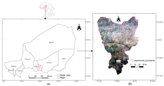
Figure 1. (a) Location of the study area, (b) Landsat 8, 2020, RGB colors.

2.2. Satellite Imagery

The Landsat 8 image was produced by the Operational Land Imager (OLI) and Thermal InfraRed Sensor (TIRS) with a revisit time of 16 days. The Sentinel-2 image was produced by the MultiSpectral Instrument (MSI) sensor, which has an orbital swath width of 290 km and a revisit time of 5 days at the Equator. Both datasets include atmospherically corrected surface reflectance. This study focused on the period from 1 October 2020, to 31 December 2020, corresponding to the end of the rainy season in the study area. During this quarter, the images are less affected by clouds, and most of the trees have leaves. Pre-processing was applied to download satellite images, which involved filtering images with more than 20% cloud cover. Then, a mask was used at the pixel level to remove the remaining clouds. Finally, the median reducer was applied to all the pixels of the image collection. In this collection, 16 Landsat 8 images and 113 Sentinel-2 images were used. This process was carried out on the Google Earth Engine (GEE) platform.

The classification is performed using visible, infrared, and shortwave infrared spectra. The bands 2, 3, 4, 5, 6, and 7 from Landsat 8 and the bands 2, 3, 4, 5, 6, 7, 8, 8A, 11, and 12 from Sentinel-2 were included as input variables. Furthermore, four other indices have been calculated to enhance classification results [43], including NDVI, Modified Normalized Difference Water Index (MNDWI), Normalized Difference Built-up Index (NDBI), and Bare Soil Index (BSI). Indices are computed as follows:

$$NDVI={\displaystyle \frac{NIR-R}{NIR+R}}$$

(1)

$$MNDWI={\displaystyle \frac{G-SWIR1}{G+SWIR1}}$$

(2)

$$NDBI={\displaystyle \frac{SWIR1-NIR}{SWIR1+NIR}}$$

(3)

$$BSI={\displaystyle \frac{\left(SWIR2+R\right)-\left(NIR+B\right)}{\left(SWIR2+R\right)+\left(NIR+B\right)}}$$

(4)

where NIR is the spectral reflectance in the near-infrared, R is the spectral reflectance in the red, G is the spectral reflectance in the green, SWIR is the spectral reflectance in the shortwave infrared, and B is the spectral reflectance in the blue.

2.3. Sampling

Machine learning algorithms need training on samples to make accurate predictions for which they have been designed [44,45]. To collect these samples, a sampling method must first be defined. Several sampling strategies exist depending on the study’s purpose [46]. The most common methods include systematic sampling, random sampling, and stratified random sampling [45]. In this study, the latter was used. Stratified random sampling allows accurate mapping of both small and large land cover units [47]. We base the stratification on the classes from the European Space Agency (ESA) World cover map 2020. This map helps to define the most predominant land cover units encountered throughout the study area. Refs. [48,49] used ESA WorldCover in stratified sampling in their studies and found that the accuracy is reliable for most land covers.

The map is accessible at: https://viewer.esa-worldcover.org/worldcover/ accessed on 18 July 2024. Thus, six land cover units were selected, including Tree/Shrub, Grassland, Cropland, Settlement, Water body, and Bare soil.

To find out the approximate sample size to be randomly distributed across each stratum, the following equation was used [50,51]:

$$n={\displaystyle \frac{Z_{\alpha /2}^2·P(1-P)}{e^2}},$$

(5)

where n is the number of plots, Z is the z-statistic at the 95% confidence level (here, $Z_{\alpha /2}$ is equal to 1.96), P is the estimated land cover proportion, and e is the acceptable margin of error. However, since the actual land cover proportion is difficult to assess, the best estimate of it is P = 50%. The margin of error is set at 5%. This acceptable level of error is reported to yield accurate results [52]. Thus, the number of plots per land cover unit will be 384. However, for the Water body unit, the value of P = 10% was used due to its very low representation in the study area. For this land cover, the plot size will therefore be set at 138. Thus, a total of 2058 plots will have to be randomly spread across the selected strata, which will be equivalent to 51,450 samples. However, given that Collect Earth Online (CEO) has an upper limit of 50,000 samples, the previous total size of the plots will be slightly adjusted accordingly. Hence, 234 plots will be distributed among Tree/Shrub, Grassland, Cropland, Settlement, and Bare soil strata, while 49 plots will be distributed in the Water body unit. This accounts for a total sample size of 1719 (Figure 2).

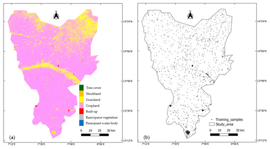
Figure 2. Stratified random sampling for collecting training samples: (a) ESA World Cover, 2020; (b) Location of training samples.

First, the sampling plan is designed in ArcGIS (10.8.1) and QGIS (3.28.7 Firenze), then imported into the CEO platform to define how each plot will be sampled. Systematic sampling will be preferred here because it provides a more accurate representation of the space explored. The plot will be 90 m wide with a square shape. This choice considers the size of a Landsat pixel, which is 30 m at the nadir, but increases and can significantly exceed this size as one moves away from nadir. In each plot, 25 training samples will be systematically distributed with 20 m spacing (Figure 3).

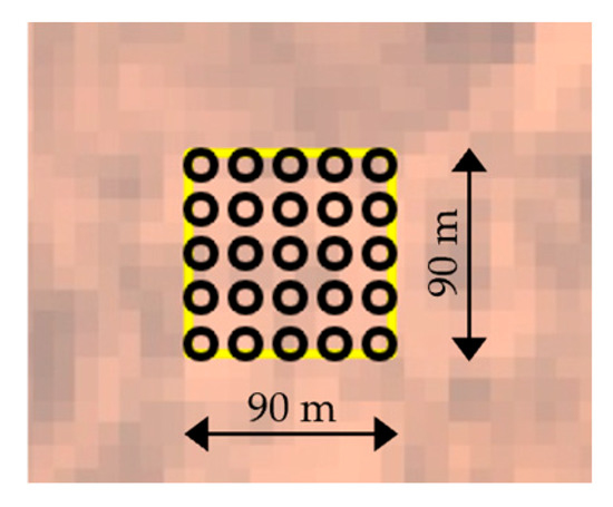
Figure 3. Distribution of training samples in a plot in CEO platform.

Therefore, the total number of training samples in the study area amounts to 42,975 (i.e., 1719 plots multiplied by 25 samples per plot) (Figure 4).

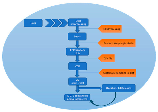
Figure 4. Sampling flowchart.

2.4. Photo Interpretation

Once the sampling strategy is defined, photo interpretation can be performed in each plot. Photo interpretation involves examining each point in the plot to decide which occupancy unit (Tree/Shrub, Grassland, Cropland, Water body, Settlement, or Bare soil) it belongs to. Consequently, this requires using available satellite images in CEO as well as images from the two sensors (Landsat 8 and Sentinel-2) for the considered period (October–December 2020). Despite the spatial resolution, interpreting a satellite image can sometimes be challenging, depending on the geographical area. Hence, due to its archival satellite imagery, Google Earth Pro can sometimes provide useful insight that can help understand the content of an image at a given point. Additionally, the CEO platform allows the computation of indices, such as the Normalized Difference Vegetation Index (NDVI), which provides further insight to ease photo interpretation [53,54].

2.5. Random Forest Parameter Tuning

The Random Forest (RF) algorithm was developed by [55]. It is part of what is called a machine learning algorithm. This term refers to algorithms capable of making predictions after being trained on a given dataset. RF can be classified as part of non-parametric statistical methods that can handle classification as well as regression problems [56,57]. Random Forest has been applied in various fields, including environmental science, natural resource management, natural risk management [58], ecology, object recognition, and bioinformatics [59], among others. It is a powerful and robust algorithm that enables image classification with greater accuracy [60,61,62].

RF is based on a set of votes for the most popular class by each randomly selected vector. It uses techniques such as bagging (bootstrap aggregating) to reduce or eliminate, in some cases, the instability of the model [55]. It can contain several trees (literally, a forest of trees), and each contributes to predicting the land cover percentage of each pixel, with the best prediction for each validation point being kept [63]. That means, in regression mode, instead of voting for a class, each tree predicts a continuous value, and the final output is the average of all predictions.

RF uses the following parameters: number of trees (ntrees), bag fraction (bf), variable per split (vps), minimum leaf population, maximum node, and seed. It has been reported that using default parameters yields reliable results [59]. However, defining the best parameters to use before performing a classification increases accuracy. In this study, we tuned the values of three main parameters: ntrees, bf, and vps (Figure 5). These values are used on both Landsat 8 and Sentinel-2 images. Likewise, RF is used in regression mode in this study. Random Forest regression (RFR) has revealed strong potential in mapping land cover, tree canopy cover, or biomass with low Root Mean Square Error, compared to other algorithms such as Support Vector Machine (SVM), Support Vector Regression (SVR), or Artificial Neural Networks (ANN) [64,65]. RFR was also used by [66] in their study to map tree canopy cover.

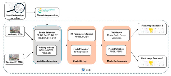
Figure 5. Methodological flowchart.

For model training, the dataset needs to be split into a training and a testing set. In the literature, percentages including 60/40 [67], 70/30 [67,68,69,70], or 80/20 [71] are commonly used for training and testing Machine Learning models. In this study, random sampling was performed, with 80% of the samples for training, whereas the remaining 20% served as the testing set.

2.6. Cross-Validation

Cross-validation determines the accuracy of a model by testing it on a dataset it has never seen before. There are several cross-validation methods, each with its advantages and drawbacks. In this study, we used Monte Carlo cross-validation (MCCV). It is a robust and effective method for a relatively large dataset [72,73]. This technique involves splitting the dataset into two groups, one for training and another for testing the model. Various types of splits are commonly found in the literature. For example, ref. [74] applied MCCV in the study of Parkinson’s disease with 60% of samples for training and 40% of samples for testing. Ref. [75] used 66% of the data for training and the remaining 33% for testing in mapping the Spartina alterniflora-invaded mangrove forest in Shankou Mangrove National Nature Reserve, in China. In his research comparing leave-one-out cross-validation to MCC, ref. [71] applied 80% and 20% of samples for training and testing, respectively. Ref. [72] tried both 66/33 and 80/20 splits to compare resampling methods for remote sensing classification in a National Park and Nature Reserve of Australia. We have used 80% of the data for training the model, and 20% was kept for validation. After each validation round, one or more metrics are computed to assess the model’s accuracy. This process is repeated several times (50 iterations in this case) for each land cover unit, and the average of the metrics is calculated to assess the accuracy. Two metrics have been computed as follows:

• Root Mean Square Error (RMSE):

$$RMSE=\sqrt{{\displaystyle \frac{1}{n}}{\sum }_{i=1}^n{\left(y_i-{\widehat{y}}_i\right)}^2},$$

(6)

• Percentage of bias (PBIAS):

  $$PBIAS={\displaystyle \frac{{\sum }_{i=1}^n\left(y_i-{\widehat{y}}_i\right)}{{\overline{y}}_i}}\ast 100,$$

  (7)

  where n is the number of predictions, $yi$ is the observed value, ${\widehat{y}}_i$ is the predicted value, and ${\overline{y}}_i$ is the mean of the observed values.

These metrics are commonly used to evaluate the accuracy of RF regression models [69,76,77,78]. The mean of each metric was tested at the 5% significance level to determine if there is a statistically significant difference between the results yielded by the two sensors. Student’s t-test was performed when the data followed a normal distribution, while the Wilcoxon test was applied when it did not.

3. Results

3.1. Comparison of Land Cover Maps

Figure 6 shows the percentage of cover predicted for the six land cover units selected according to the sensor type (Landsat 8 or Sentinel-2). Grassland and cropland land covers have good spatial representation, followed, to a lesser extent, by the tree/shrub land cover (Figure 6). The bias is generally low (gray points) for the tree/shrub land cover and both sensors (Figure 6a,b). For the grassland and cropland land covers, the bias is relatively higher (red and blue points) (Figure 6c–f). However, it remains generally low over the study area.

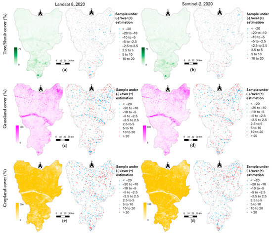
Figure 6. Predicted land cover units and absolute bias for Landsat 8 and Sentinel-2, 2020: (a) Tree/shrub, Landsat 8; (b) Tree/Shrub, Sentinel-2; (c) Grassland, Landsat 8; (d) Grassland, Sentinel-2; (e) Cropland, Landsat 8; (f) Cropland, Sentinel-2.

It is worth mentioning that, although it exists, the difference in percentage coverage between the two sensors remains globally low.

Figure 7 shows the percentage cover for settlement, water body, and bare soil land covers, along with the corresponding absolute bias for each sensor. The settlement land cover has been accurately mapped by both sensors, despite the settlements being widely scattered across the study area (Figure 7a,b). Although it has a small spatial extent, the water body unit was still detected by both sensors (Figure 7c,d). Bare soils were also well represented by each sensor. However, when comparing the two sensors, the difference in the percentage cover is barely perceptible.

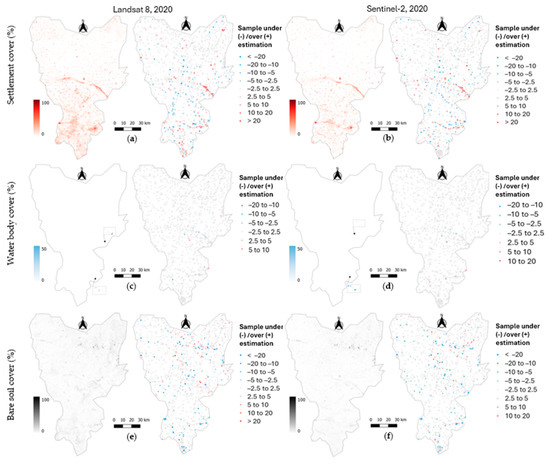
Figure 7. Predicted land cover units and absolute bias for Landsat 8 and Sentinel-2, 2020: (a) Settlement, Landsat 8; (b) Settlement, Sentinel-2; (c) Water body, Landsat 8; (d) Water body, Sentinel-2; (e) Bare soil, Landsat 8; (f) Bare soil, Sentinel-2.

The overall bias is also quite low (gray dots), especially for the water body unit (Figure 7c,d). However, some substantial values were noticeable where the model tends to overestimate (red dots) and occasionally underestimate (blue dots) (Figure 7a,b,e,f). Whether it is the percentage cover or the bias produced, the difference between the two sensors remains small.

Table 1 summarizes the estimated areas for each land cover according to the sensor type. The areas determined by the model for Sentinel-2 are lower than those evaluated for Landsat 8, except for the cropland land cover. Indeed, the Sentinel-2 sensor can determine up to 4% more cropland than the Landsat 8 sensor.

Table 1. Comparison of area occupancy by sensor type.

Sensor	Landsat 8 (L8)		Sentinel-2 (S2)		Difference S2-L8 (%)
Land Cover	Absolute (km2)	Relative (%)	Absolute (km2)	Relative (%)
Tree/Shrub	424.59	5.09	404.91	4.86	−0.23
Grassland	1352.51	16.21	1223.18	14.67	−1.54
Cropland	6111.42	73.23	6433.27	77.17	3.94
Settlement	247.76	2.97	140.51	1.69	−1.28
Waterbody	5.41	0.06	2.55	0.03	−0.03
Bare soil	203.81	2.44	132.55	1.59	−0.85
Total	8346	100	8337	100

3.2. Pixel-Based Comparison

Figure 8 shows maps of pixel-based differences in percentage cover between Sentinel-2 and Landsat 8. This difference is noticeable throughout the entire study area for grassland and cropland (Figure 8b,c). Pixels resulting from this difference are mostly negative for grassland, meaning Landsat 8 estimates more grass than Sentinel-2. Conversely, for cropland, the pixels are mostly positive, indicating Sentinel-2 estimates more cropland than Landsat 8. This difference is near zero for other land cover types, except in the southern part of the study area for the tree/shrub and settlement land covers (Figure 8a,d). For water bodies, some values exceeding 5% in absolute value are spotted in the center of the study area (Figure 8e).

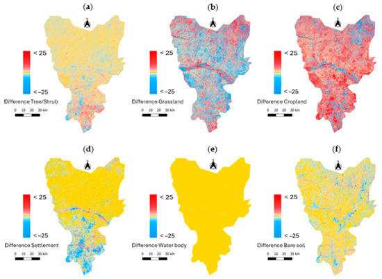
Figure 8. Pixel-based differences in percentage cover between Sentinel-2 and Landsat 8 (i.e., Sentinel-2 percent cover map—Landsat 8 percent cover map) across all land covers: (a) Tree/Shrub; (b) Grassland; (c) Cropland; (d) Settlement; (e) Water body; (f) Bare soil.

In Appendix A, the pixel-based cumulative distribution functions of percentage cover have been plotted as a function of the sensor. For each cover type, a small difference is observed between the two curves. In other words, the distribution functions between Sentinel-2 and Landsat 8 do not fit perfectly throughout the curve. This difference is more easily observed for grassland, cropland, settlement, and bare soil (Figure A1b–e). The figures highlight that there is a difference between the results yielded by the two sensors, but this difference remains very small.

The pixel-based histogram of the differences in the percentage cover is shown in Figure 9. It can also be observed that the histogram is not perfectly symmetrical around the red dotted line, which represents the symmetrical axis. This information suggests a very small difference between the areas estimated by the two sensors. Moreover, it can also be noticed that the pixel-based differences in the percentage cover (i.e., Sentinel-2 map—Landsat 8 map) are negative for tree/shrub, grassland, settlement, bare soil, and water body (Figure 9a,b,d–f), whereas they are positive for the Cropland (Figure 9c).

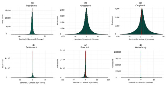
Figure 9. Histogram of the pixel-based differences in percentage cover between Sentinel-2 and Landsat 8 (i.e., Sentinel-2 percent cover map—Landsat 8 percent cover map) across all land covers: (a) Tree/Shrub; (b) Grassland; (c) Cropland; (d) Settlement; (e) Bare soil; (f) Waterbody.

To identify potential differences between the areas assessed by the two sensors, the Kolmogorov–Smirnov test was performed to compare the shapes of the cumulative distribution functions. The test is significant for all six land cover types at p < 0.001, indicating that the cumulative distribution functions from Landsat 8 and Sentinel-2 are different. In addition, the Wilcoxon test shows that the median of the pixel-based differences in percentage cover between the two sensors is different from zero (p < 0.001) (Table 2). This result indicates that the medians of the pixel-based percentage cover differences between the two sensors are statistically different.

Table 2. Comparison of the median of pixel-based difference in percentage cover between Sentinel-2 and Landsat 8 (i.e., Sentinel-2 percent cover map—Landsat 8 percent cover map).

	Pixel-Based Differences Cover (%)
Land Cover	Mean	Median	Wilcoxon Test
Tree/Shrub	−0.24	−0.20	***
Grassland	−1.57	−1.83	***
Cropland	3.81	3.56	***
Settlement	−1.29	−0.02	***
Waterbody	−0.03	0.003	***
Bare soil	−0.86	−0.44	***

*** p-value < 0.001.

3.3. Validation Results

The cropland unit recorded the highest RMSE, followed by grassland, settlement, bare soil, tree/shrub, and water body. Sentinel-2 yielded the lower RMSE for all land covers except for the water body unit, where the opposite is observed. However, this difference is statistically significant at p < 0.05, including for the water body unit (Figure 10a). Although statistically significant, this difference between the two sensors remains small.

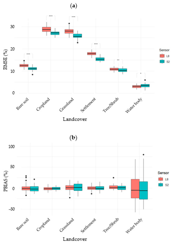
Figure 10. Metrics comparison by land cover and sensor type: (a) Root mean square error; (b) Percent bias. *: p-value < 0.05; **: p-value < 0.01; ***: p-value < 0.001.

The systematic error produced by both sensors is almost zero, except for the water body unit, where it is relatively high (Figure 10b). Moreover, the Sentinel-2 sensor exhibited a lower bias than the Landsat 8 sensor in the bare soil, settlement, tree/shrub, and water body units. Conversely, for the cropland and grassland units, Landsat 8 yielded the lowest bias. However, it should be highlighted that for all land covers, the difference observed in percent bias between the two sensors is not significant at p < 0.05.

4. Discussion

4.1. The Importance of Regression-Based Land Cover Mapping Using a Cloud Platform

Most land cover mapping using satellite images employs discrete categories, meaning the presence or absence of a specific cover within a pixel, which is a simplification of reality. This approach works well for mapping forests or dense vegetation areas. However, in patchy landscapes, such as agropastoral Sahelian regions, this representation may not be suitable due to within-pixel land cover heterogeneity [79]. This issue is further exacerbated when using medium-resolution satellite images, as it may increase bias [80]. It can be addressed by using the fractional cover of each class within a pixel. Instead of categorical classification, fractional cover more accurately captures heterogeneity or patchiness. In this regard, ref. [81] confirmed that a continuous land cover scheme represents heterogeneous areas more efficiently than the standard categorical classification scheme. For example, RFR is a widely used and robust method for continuous land cover mapping [64,65,66,67,68,69,70,79,80,81]. However, RFR is generally more computationally intensive than RF classification (categorical analysis). To address this challenge, we ran the RFR analysis using the GEE platform, which is known for handling intensive computational tasks with large-scale satellite imagery [82,83,84]. Moreover, GEE allows a wide range of pre-processing and advanced analytical tools without concerns about storage capacity or processing speed. In the context of climate change and rapidly growing data volumes, GEE appears to be an important platform that can support academic institutions, research centers, and environmental managers in decision-making, especially in developing countries.

4.2. The Importance of Spatial and Spectral Resolution in Land Cover Mapping

Satellite images enable Land Use Land Cover (LULC) analyses to be performed with reliable accuracy. The availability of Landsat and Sentinel satellite imagery helps achieve this objective, depending on the required spatial resolution. This is one of the main limitations in producing accurate LULC maps. Sentinel imagery has addressed this issue by providing free access to images with a 10 m spatial resolution (for the visible bands), which is three times better than what Landsat imagery provides. Very high-resolution satellite images are also available, such as Planet imagery, which has a spatial resolution of 4.77 m, but these images are not publicly accessible.

However, when it comes to performing a temporal analysis, one can quickly face limitations depending on the sensor choice. For Sentinel, the first image available started in 2014 (with Sentinel-1A), so analyses on this sensor cannot go beyond this date. On the other hand, the Landsat sensor goes further back, since the first Landsat image was acquired in 1972 (with the Earth Resources Technology Satellite).

This study revealed a difference between the Landsat 8 and Sentinel-2 results. This difference is highlighted mostly in Figure 8b–d. The cumulative distribution functions (Figure A1) also show a difference in shape, especially for grassland, cropland, settlement, and, to a lesser extent, bare soil. These differences in shape are significant at p < 0.001. The validation results show that the RMSE yielded by the two sensors is significant at p < 0.05, underlining that there is a difference in how each sensor estimates the land cover. Since the difference is significant, it indicates that the two sensors estimate a given land cover differently, mainly due to the spatial resolution difference. Indeed, while Landsat 8 faces challenges with pixels that may include two or more land covers due to the patchy landscape of the study area, Sentinel-2 delivers better results because its smaller pixels reduce mixing. Effective mapping of patchy landscapes requires high-resolution sensors, as spatial resolution contributes to the overall accuracy. In this case, Landsat 8 tends to produce more mixed pixels compared to Sentinel-2 due to the difference in spatial resolution.

The spectral resolution of a sensor is its ability to differentiate low energy levels in the electromagnetic spectrum. It refers to both bandwidth and the number of spectral bands in which the sensor captures information about Earth materials. The finer the spectral band, the more subtle differences the sensor can detect, allowing it to better identify objects on the Earth’s surface. In fact, between 635 and 885 nanometers, the Sentinel-2 sensor has six spectral bands (Red, Red edge, Band 6 with a central wavelength of 740 nanometers, Band 7 with a central wavelength of 783 nanometers, Band 8 (NIR), and Band 8A with a central wavelength of 865 nanometers), all of which help improve vegetation classification. In comparison, Landsat 8 has only two bands (Red and NIR) within approximately the same wavelength range (636–879 nanometers). This improvement in spectral resolution in this wavelength range allows Sentinel-2 to better capture subtle differences that Landsat 8 may miss. Consequently, Sentinel-2 yields lower RMSE and PBIAS values compared to Landsat 8. Despite the difference in the number of spectral bands used in this study, Sentinel-2’s performance appears to be slightly higher than that of Landsat 8. This outcome is similar to the studies of [85,86], who found that Sentinel-2 outperformed Landsat 8 even when near-equivalent image bands were used and Sentinel-2 was down-sampled to a spatial resolution of 30 m. Furthermore, assessing the classification accuracies for LULC mapping in Istanbul, ref. [87] achieved an overall accuracy of 70.60% with Landsat 8 and 76.40% with Sentinel-2 using the Maximum Likelihood Classification (MLC) method. Using the Support Vector Machine (SVM) approach, accuracy increased to 81.67% for Landsat 8 and 84.17% for Sentinel-2. Since similar spectral bands were employed, they therefore concluded that spatial resolution was a key factor contributing to the higher accuracy obtained with Sentinel-2.

4.3. Analysis of Percentage Cover and Bias

The highest percentage cover of tree/shrub is found in the southern part of the study area, which is the Aguié department (Figure 6a,b). This corresponds to the highest rainfall gradient. Indeed, in Niger, rainfall increases from north to south. The density of trees and shrubs is therefore correlated with the rainfall gradient. The two sensors clearly illustrate this pattern.

In the study area, the most widespread land covers are cropland and grassland, regardless of sensor type (Figure 6c–f). Indeed, agriculture and livestock are among the main livelihood activities of the local population. Additionally, grasslands are mainly found in the center of the study area, along the seasonal watercourse, but also further north. The northern part borders the Sahelian zone, which has more grasslands and is therefore better suited for livestock farming. In fact, the Sahel stretches from the Atlantic Ocean at the Senegalese and Mauritanian coasts to the Red Sea at the Eritrean coasts. It serves as the transition zone between the Sahara in the north and the more humid regions in the south [88]. It hosts most of the livestock in the countries it crosses due to the presence of rangeland and high-quality forage [89].

Settlements are more compact in the southern part of the study area (Figure 7a,b). Indeed, the administrative units are more densely packed in the Aguié department, which has a population density of 184 inhabitants/Km² in 2024. This is significantly higher than the national average density of the country, which is 21 inhabitants/Km² in 2024. Conversely, in the northern part, the Mayahi department, which is larger than Aguié, is made up of smaller and more dispersed administrative units. As a result, the population density is lower (79 inhabitants/Km²). The model clearly captured this pattern through both sensors. Nevertheless, the bias was not statistically significant in this study, in line with the results reported by [85], which demonstrated that there is no statistical significance between Sentinel-2 and Landsat 8’s relative bias.

4.4. Analysis of the Estimated Area by the Model for Each Sensor

As expected, spatial resolution has a positive impact on the land cover mapping. High-resolution satellite imagery increases image classification accuracy and yields lower relative errors, as shown in Figure 10a, between the Landsat 8 and Sentinel-2 sensors.

Table 1 shows that Sentinel-2 could determine up to 4% (322 km²) more cropland compared to the Landsat 8 sensor. Indeed, farms often consist of small to even tiny family plots. Because Sentinel-2 has a finer spatial resolution than Landsat 8, it allows for the detection of small agricultural plots, which often border villages or dwellings, as well as corridors and rangeland areas. In Table 1, minor discrepancies in total area between Landsat, Sentinel-2, and vector-based estimates arise from raster discretization of polygon boundaries, differences in native spatial resolution, and pixel grid alignment. The observed differences are very small (<0.30%) in pixel-based area calculations.

In the study area, settlements mainly consist of widely dispersed villages and hamlets. Trees and shrubs are scattered throughout, except for a few rare groups located in the southern part of the study area (Figure 6a,b). Permanent water bodies are absent in the study area. Nevertheless, some small water bodies remain at the end of the rainy season. Bare soil includes barren upland, hardened areas, and quarries. Grassland cover includes rangeland areas, narrow cattle corridors, and a few fallows. Because Landsat 8 has a medium spatial resolution (30 m), it struggles to distinguish small neighboring land covers. Moreover, edge artifacts may lead to an overestimation of areas by Landsat 8. As a result, the estimated areas for tree/shrub, grassland, settlement, water body, and bare soil are slightly larger with Landsat 8 compared to Sentinel-2, which provides more precise measurements (Table 1) due to its finer spatial resolution. Indeed, in mapping the Spartina alterniflora-invaded mangrove in China, ref. [75] found that Sentinel-2 imagery yielded lower accuracy compared to WorldView-2 imagery, a 2 m spatial resolution imagery, highlighting the effect of spatial resolution on the overall map accuracy.

The pixel-based cumulative distribution functions (Appendix A) and the histogram of the differences in percentage cover (Figure 9) show that the estimated areas from both sensors are different. Additionally, Wilcoxon tests support this finding with p < 0.001 for all land covers (Table 2). However, the difference in the estimated areas between the two sensors remains small, with overall differences of 3.94% for cropland, 1.54% for grassland, 1.28% for settlement, 0.85% for bare soil, 0.23% for tree/shrub, and only 0.03% for water body (Table 1). The validation results show that both sensors produce similar results, although Sentinel-2 yielded slightly lower RMSE (Figure 10a). These findings suggest that Landsat 8 and Sentinel-2 produce similar image classifications.

Appendix B illustrates some differences in land cover estimates. It highlights the accuracy of the two sensors by examining some details resulting from land cover differences. Figure A2 shows a detail in grassland estimation. In (a), it shows an overestimation of this land cover by Landsat 8 (shown in blue), while the satellite image shows cropland. The detail in (b) also indicates that the area (shown in blue), which Landsat 8 identified as grassland, is currently made up of cropland on the satellite image. Another example is highlighted by Figure A3, which illustrates a detail in the estimation of tree/shrub cover. It shows that Sentinel-2 provides a more accurate estimate by clearly excluding settlements in this area, unlike the Landsat 8 sensor, where this distinction is less obvious. Indeed, the detail in Figure A4 shows that the entire area was classified by Sentinel-2 as cropland (shown in red), with small patches of grass or fallow land. This is clearly shown in the satellite image. However, some scattered settlements are also visible on the satellite image, located among the cropland in the southern part.

In land cover mapping and related mapping applications in agropastoral environments, using Sentinel-2 or Landsat 8 will yield acceptable results since the observed difference between the two sensors is small (3.94% for cropland), which is the largest observed difference among the land covers considered in this study. Therefore, Landsat 8 is an interesting product to use by policymakers or other key stakeholders for long-term land monitoring when higher-resolution products are unavailable. Nevertheless, although the differences are very small in terms of land cover mapping performance, policymakers would still benefit from higher-resolution products (such as Sentinel-2) when it comes to setting up targeted and spatially detailed land management activities.

4.5. Limitations and Perspective

In this study, the number of spectral bands varies slightly between the two sensors. Therefore, the observed Sentinel-2 performance is likely not solely due to spatial resolution but may also be influenced by differences in the number of spectral bands used in the model. Future studies could assess in detail the relative contribution of spatial and spectral resolution to overall map accuracy, particularly to determine to what extent the performance gain is attributable to one or the other resolution. Additionally, the current sampling design may limit Sentinel-2 from expressing its main advantage, which is fine spatial detail, leading to lower performance. A nested sampling design could help address scale dependence in land cover representation. Indeed, while fine-scale subplots capture spatial heterogeneity relevant to Sentinel-2, aggregated plots will provide a common evaluation scale for comparison with Landsat 8. In this study, we used 1719 plots following the approach of [51], based on a stratified random sampling design utilizing an existing global land cover map (ESA WorldCover 2020). Therefore, using a more accurate global map and/or increasing the number of plots per stratum are potential ways to further improve the current methodology and land cover maps. Furthermore, employing more powerful computers would allow for more iterations in the MCCV approach, resulting in a better assessment of map uncertainty. Another methodological improvement could be the normalization of pixel-wise values, which was not done in this study. Consequently, pixel values across all land covers did not always sum up exactly to 100%, which may influence the total area coverage. However, in this case, this effect was very small (considering all the pixels, this sum is normally distributed and centered around 100%) and did not affect the outcomes of the present study. Nonetheless, it is generally recommended to perform the normalization before any comparison for area assessment.

5. Conclusions

In this study, Landsat 8 and Sentinel-2 images acquired between October and December 2020 were classified using Random Forest regression on the Google Earth Engine platform. A total of 1719 training points were collected through stratified random sampling with the Collect Earth Online platform to train the model. Additionally, NDVI, MNDWI, NDBI, and BSI were included as variables to enhance the model’s prediction accuracy.

The study revealed that the estimated total land cover areas show differences between the two sensors. Landsat 8 estimates are higher than Sentinel-2 for all land covers except for cropland, where Sentinel-2 yielded about 4% more cropland than Landsat 8. These area differences are statistically significant at p < 0.001, although they are small. Furthermore, the performance of Sentinel-2 land cover maps is better than that of Landsat 8, with significantly lower RMSE (p < 0.05).

Hence, higher spatial resolution is likely to result in better land cover mapping accuracy. However, the greater number of spectral bands in Sentinel-2 can also contribute to better performance when using this product for land cover mapping. Since this difference is rather small (0.03–3.94%), Landsat imagery can still deliver satisfactory classification results in remote agropastoral environments with heterogeneous landscapes. These findings could be extended to other agropastoral areas of the Sahelian countries.

References

- Anand, S.; Kumar, H.; Kumar, P.; Kumar, M. Analyzing landscape changes and their relationship with land surface temperature and vegetation indices using remote sensing and AI techniques. Geosci. Lett. 2025, 12, 7. [Google Scholar] [CrossRef]
- Guo, Q.; Han, L.; Li, L.; Qu, S. Refining historical forest cover mapping and change analysis with time series algorithm-based samples transfer. Phys. Chem. Earth 2025, 139, 103893. [Google Scholar] [CrossRef]
- Zhu, Z.; Qiu, S.; Ye, S. Remote sensing of land change: A multifaceted perspective. Remote Sens. Environ. 2022, 282, 113266. [Google Scholar] [CrossRef]
- Sammartino, M.; Buongiorno Nardelli, B.; Marullo, S.; Santoleri, R. An Artificial Neural Network to Infer the Mediterranean 3D Chlorophyll-a and Temperature Fields from Remote Sensing Observations. Remote Sens. 2020, 12, 4123. [Google Scholar] [CrossRef]
- Albugami, S.; Palmer, S.; Cinnamon, J.; Meersmans, J. Spatial and Temporal Variations in the Incidence of Dust Storms in Saudi Arabia Revealed from In Situ Observations. Geosciences 2019, 9, 162. [Google Scholar] [CrossRef]
- Elshukri, F.; Abusirriya, N.H.; Braganza, N.J.; Amhamed, A.; Alrebei, O.F. Temporal and spatial pattern analysis and forecasting of methane: Satellite image processing. Ecol. Inform. 2025, 89, 103176. [Google Scholar] [CrossRef]
- Garba, I.; Amadou, S.A.; Barry, B.; Ouedraogo, S. Suivi des feux de brousse en Afrique de l’Ouest et au Sahel, un outil d’aide à la décision. Int. J. Biol. Chem. Sci. 2021, 15, 2636–2651. [Google Scholar] [CrossRef]
- Kariuki, N.G.; Chiawo, D.O.; Kairu, E.W.; Simbauni, J.A.; Muthiuru, A.C. Weather pattern and wildfire interplay in Tsavo Conservation Area, Kenya. Fire Ecol. 2025, 21, 18. [Google Scholar] [CrossRef]
- Ezzine, A.; Saidi, S.; Hermassi, T.; Kammessi, I.; Darragi, F.; Rajhi, H. Flood mapping using hydraulic modeling and Sentinel-1 image: Case study of Medjerda Basin, northern Tunisia. Egypt. J. Remote Sens. Space Sci. 2020, 23, 303–310. [Google Scholar] [CrossRef]
- Sommer, S.; Hill, J.; Mégier, J. The potential of remote sensing for monitoring rural land use changes and their effects on soil conditions. Agric. Ecosyst. Environ. 1998, 67, 197–209. [Google Scholar] [CrossRef]
- Mariano, D.A.; dos Santos, C.A.; Wardlow, B.D.; Anderson, M.C.; Schiltmeyer, A.V.; Tadesse, T.; Svoboda, M.D. Use of remote sensing indicators to assess effects of drought and human-induced land degradation on ecosystem health in Northeastern Brazil. Remote Sens. Environ. 2018, 213, 129–143. [Google Scholar] [CrossRef]
- Li, X.; Gong, P.; Liang, L. A 30-year (1984–2013) record of annual urban dynamics of Beijing City derived from Landsat data. Remote Sens. Environ. 2015, 166, 78–90. [Google Scholar] [CrossRef]
- Mirsanjari, M.M.; Zarandian, A.; Mohammadyari, F.; Visockiene, J.S. Investigation of the impacts of urban vegetation loss on the ecosystem service of air pollution mitigation in Karaj metropolis, Iran. Environ. Monit. Assess. 2020, 192, 501. [Google Scholar] [CrossRef]
- Hirschmugl, M.; Deutscher, J.; Sobe, C.; Bouvet, A.; Mermoz, S.; Schardt, M. Use of SAR and Optical Time Series for Tropical Forest Disturbance Mapping. Remote Sens. 2020, 12, 727. [Google Scholar] [CrossRef]
- Zhao, M.; Zhou, Y.; Li, X.; Cheng, W.; Zhou, C.; Ma, T.; Li, M.; Huang, K. Mapping urban dynamics (1992–2018) in Southeast Asia using consistent nighttime light data from DMSP and VIIRS. Remote Sens. Environ. 2020, 248, 111980. [Google Scholar] [CrossRef]
- Samarin, M.; Zweifel, L.; Roth, V.; Alewell, C. Identifying Soil Erosion Processes in Alpine Grasslands on Aerial Imagery with a U-Net Convolutional Neural Network. Remote Sens. 2020, 12, 4149. [Google Scholar] [CrossRef]
- Xu, Z.; Wang, Y. Radar Satellite Image Time Series Analysis for High-Resolution Mapping of Man-Made Forest Change in Chongming Eco-Island. Remote Sens. 2020, 12, 3438. [Google Scholar] [CrossRef]
- Mobarakeh, Z.M.; Pourmanafi, S.; Ahmadi, M. Employing Sentinel-2 time-series and noisy data quality control enhance crop classification in arid environments: A comparison of machine learning and deep learning methods. Int. J. Appl. Earth Obs. Geoinf. 2025, 142, 104678. [Google Scholar] [CrossRef]
- Baillarin, S.J.; Meygret, A.; Dechoz, C.; Petrucci, B.; Lacherade, S.; Tremas, T.; Isola, C.; Martimort, P.; Spoto, F. Sentinel-2 Level 1 Products and Image Processing Performances. Int. Arch. Photogramm. Remote Sens. Spat. Inf. Sci. 2012, XXXIX-B1, 197–202. [Google Scholar] [CrossRef]
- Drusch, M.; Del Bello, U.; Carlier, S.; Colin, O.; Fernandez, V.; Gascon, F.; Hoersch, B.; Isola, C.; Laberinti, P.; Martimort, P.; et al. Sentinel-2: ESA’s Optical High-Resolution Mission for GMES Operational Services. Remote Sens. Environ. 2012, 120, 25–36. [Google Scholar] [CrossRef]
- Immitzer, M.; Vuolo, F.; Atzberger, C. First Experience with Sentinel-2 Data for Crop and Tree Species Classifications in Central Europe. Remote Sens. 2016, 8, 166. [Google Scholar] [CrossRef]
- Vuolo, F.; Żółtak, M.; Pipitone, C.; Zappa, L.; Wenng, H.; Immitzer, M.; Weiss, M.; Baret, F.; Atzberger, C. Data Service Platform for Sentinel-2 Surface Reflectance and Value-Added Products: System Use and Examples. Remote Sens. 2016, 8, 938. [Google Scholar] [CrossRef]
- Roy, D.P.; Wulder, M.A.; Loveland, T.R.; Woodcock, C.E.; Allen, R.G.; Anderson, M.C.; Helder, D.; Irons, J.R.; Johnson, D.M.; Kennedy, R.; et al. Landsat-8: Science and product vision for terrestrial global change research. Remote Sens. Environ. 2014, 145, 154–172. [Google Scholar] [CrossRef]
- Gorelick, N.; Hancher, M.; Dixon, M.; Ilyushchenko, S.; Thau, D.; Moore, R. Google Earth Engine: Planetary-scale geospatial analysis for everyone. Remote Sens. Environ. 2017, 202, 18–27. [Google Scholar] [CrossRef]
- Bastin, J.-F.; Berrahmouni, N.; Grainger, A.; Maniatis, D.; Mollicone, D.; Moore, R.; Patriarca, C.; Picard, N.; Sparrow, B.; Abraham, E.M.; et al. The extent of forest in dryland biomes. Science 2017, 356, 635–638. [Google Scholar] [CrossRef]
- Shelestov, A.; Lavreniuk, M.; Kussul, N.; Novikov, A.; Skakun, S. Exploring Google Earth Engine Platform for Big Data Processing: Classification of Multi-Temporal Satellite Imagery for Crop Mapping. Front. Earth Sci. 2017, 5, 232994. [Google Scholar] [CrossRef]
- Saah, D.; Johnson, G.; Ashmall, B.; Tondapu, G.; Tenneson, K.; Patterson, M.; Poortinga, A.; Markert, K.; Quyen, N.H.; Aung, K.S.; et al. Collect Earth: An online tool for systematic reference data collection in land cover and use applications. Environ. Model. Softw. 2019, 118, 166–171. [Google Scholar] [CrossRef]
- Bey, A.; Díaz, A.S.-P.; Maniatis, D.; Marchi, G.; Mollicone, D.; Ricci, S.; Bastin, J.-F.; Moore, R.; Federici, S.; Rezende, M.; et al. Collect Earth: Land Use and Land Cover Assessment through Augmented Visual Interpretation. Remote Sens 2016, 8, 807. [Google Scholar] [CrossRef]
- Agassounon, B.M.; Assede, E.S.P.; Bastin, J.-F.; Biaou, S.S.H. Remote sensing applied in land use and land cover change (LUCC) in arid and semi-arid ecosystems: Current status, challenges and prospects—A systematic review. Environ. Monit. Assess. 2025, 197, 1266. [Google Scholar] [CrossRef] [PubMed]
- Ramalason, F.N.; Rakotondrasoa, O.L.; Linden, A.V.; Renard, G.; Ratsimba, H.R.; Bogaert, J.; Bastin, J.-F. Potential of global vegetation maps in capturing xerophytic vegetation cover: Insights from Madagascar’s arid ecosystems. J. Arid Environ. 2025, 229, 105406. [Google Scholar] [CrossRef]
- Irons, J.R.; Markham, B.L.; Nelson, R.F.; Toll, D.L.; Williams, D.L.; Latty, R.S.; Stauffer, M.L. The effects of spatial resolution on the classification of Thematic Mapper data. Int. J. Remote Sens. 1985, 6, 1385–1403. [Google Scholar] [CrossRef]
- Cushnie, J.L. The interactive effect of spatial resolution and degree of internal variability within land-cover types on classification accuracies. Int. J. Remote Sens. 1987, 8, 15–29. [Google Scholar] [CrossRef]
- Hsieh, P.-F.; Lee, L.C.; Chen, N.-Y. Effect of spatial resolution on classification errors of pure and mixed pixels in remote sensing. IEEE Trans. Geosci. Remote Sens. 2001, 39, 2657–2663. [Google Scholar] [CrossRef]
- Hu, Z.; Chu, Y.; Zhang, Y.; Zheng, X.; Wang, J.; Xu, W.; Wang, J.; Wu, G. Scale matters: How spatial resolution impacts remote sensing based urban green space mapping? Int. J. Appl. Earth Obs. Geoinf. 2024, 134, 104178. [Google Scholar] [CrossRef]
- Pleniou, M.; Koutsias, N. The role of spectral vs spatial resolution of satellite data on the accuracy of mapping unburned vegetation within fire scar perimeters. Sci. Remote Sens. 2025, 11, 100241. [Google Scholar] [CrossRef]
- Fisher, J.R.B.; Acosta, E.A.; Dennedy-Frank, P.J.; Kroeger, T.; Boucher, T.M. Impact of satellite imagery spatial resolution on land use classification accuracy and modeled water quality. Remote Sens. Ecol. Conserv. 2018, 4, 137–149. [Google Scholar] [CrossRef]
- Chen, D.; Stow, D.A.; Gong, P. Examining the effect of spatial resolution and texture window size on classification accuracy: An urban environment case. Int. J. Remote Sens. 2004, 25, 2177–2192. [Google Scholar] [CrossRef]
- Campos, J.C.; Brito, J.C. Mapping underrepresented land cover heterogeneity in arid regions: The Sahara-Sahel example. ISPRS J. Photogramm. Remote Sens. 2018, 46, 211–220. [Google Scholar] [CrossRef]
- Brandt, M.; Hiernaux, P.; Rasmussen, K.; Mbow, C.; Kergoat, L.; Tagesson, T.; Ibrahim, Y.Z.; Wélé, A.; Tucker, C.J.; Fensholt, R. Assessing woody vegetation trends in Sahelian drylands using MODIS-based seasonal metrics. Remote Sens. Environ. 2016, 183, 215–225. [Google Scholar] [CrossRef]
- Diouf, A.; Lambin, E.F. Monitoring land-cover changes in semi-arid regions: Remote sensing data and field observations in the Ferlo, Senegal. J. Arid Environ. 2001, 48, 129–148. [Google Scholar] [CrossRef]
- Abdel Kader, H.S. Évaluation des Ressources en eau de l’Aquifère du Continental Intercalaire/Hamadien de la Région de Tahoua (Bassin des Iullemeden, Niger): Impacts Climatiques et Anthropiques. Géochimie. Ph.D. Thesis, Université Paris-Saclay, Orsay, France, Université de Niamey, Niamey, Niger, 2018. Available online: https://tel.archives-ouvertes.fr/tel-02089629 (accessed on 28 July 2025).
- Niger National Institute of Statistics. Available online: https://www.stat-niger.org/projections/ (accessed on 10 June 2025).
- Hermosilla, T.; Wulder, M.A.; White, J.C.; Coops, N.C. Land cover classification in an era of big and open data: Optimizing localized implementation and training data selection to improve mapping outcomes. Remote Sens. Environ. 2022, 268, 112780. [Google Scholar] [CrossRef]
- Ng, W.; Minasny, B.; Mendes, W.d.S.; Demattê, J.A.M. The influence of training sample size on the accuracy of deep learning models for the prediction of soil properties with near-infrared spectroscopy data. SOIL 2020, 6, 565–578. [Google Scholar] [CrossRef]
- Shetty, S.; Gupta, P.K.; Belgiu, M.; Srivastav, S.K. Assessing the Effect of Training Sampling Design on the Performance of Machine Learning Classifiers for Land Cover Mapping Using Multi-Temporal Remote Sensing Data and Google Earth Engine. Remote Sens. 2021, 13, 1433. [Google Scholar] [CrossRef]
- Cochran, W.G. Sampling Techniques, 3rd ed.; John Wiley & Sons: New York, NY, USA, 1977; pp. 89–110. [Google Scholar]
- Congalton, R.G. A Comparison of Sampling Schemes Used in Generating Error Matrices for Assessing the Accuracy of Maps Generated from Remotely Sensed Data. Photogramm. Eng. Remote Sens. 1988, 54, 593–600. [Google Scholar]
- Chaaban, F.; El Khattabi, J.; Darwishe, H. Accuracy Assessment of ESA WorldCover 2020 and ESRI 2020 Land Cover Maps for a Region in Syria. J. Geovis. Spat. Anal. 2022, 6, 31. [Google Scholar] [CrossRef]
- Venter, Z.S.; Barton, D.N.; Chakraborty, T.; Simensen, T.; Singh, G. Global 10 m Land Use Land Cover Datasets: A Comparison of Dynamic World, World Cover and Esri Land Cover. Remote Sens. 2022, 14, 4101. [Google Scholar] [CrossRef]
- Fitzpatrick-Lins, K. Comparison of Sampling Procedures and Data Analysis for a Land-Use and Land-Cover Map. Photogramm. Eng. Remote Sens. 1981, 47, 343–351. [Google Scholar]
- Foody, G.M. Sample size determination for image classification accuracy assessment and comparison. Int. J. Remote Sens. 2009, 30, 5273–5291. [Google Scholar] [CrossRef]
- Sarvia, F.; De Petris, S.; Borgogno-Mondino, E. Mapping Ecological Focus Areas within the EU CAP Controls Framework by Copernicus Sentinel-2 Data. Agronomy 2022, 12, 406. [Google Scholar] [CrossRef]
- Lamchin, M.; Lee, J.-Y.; Lee, W.-K.; Lee, E.J.; Kim, M.; Lim, C.-H.; Choi, H.-A.; Kim, S.-R. Assessment of land cover change and desertification using remote sensing technology in a local region of Mongolia. Adv. Space Res. 2016, 57, 64–77. [Google Scholar] [CrossRef]
- Kumar, B.P.; Babu, K.R.; Anusha, B.; Rajasekhar, M. Geo-environmental monitoring and assessment of land degradation and desertification in the semi-arid regions using Landsat 8 OLI/TIRS, LST, and NDVI approach. Environ. Chall. 2022, 8, 100578. [Google Scholar] [CrossRef]
- Breiman, L. Random Forests. Mach. Learn. 2001, 45, 5–32. [Google Scholar] [CrossRef]
- Immitzer, M.; Atzberger, C.; Koukal, T. Tree Species Classification with Random Forest Using Very High Spatial Resolution 8-Band WorldView-2 Satellite Data. Remote Sens. 2012, 4, 2661–2693. [Google Scholar] [CrossRef]
- Genuer, R.; Poggi, J.-M.; Tuleau-Malot, C.; Villa-Vialaneix, N. Random Forests for Big Data. Big Data Res. 2017, 9, 28–46. [Google Scholar] [CrossRef]
- Talukdar, S.; Singha, P.; Mahato, S.; Shahfahad Pal, S.; Liou, Y.-A.; Rahman, A. Land-Use Land-Cover Classification by Machine Learning Classifiers for Satellite Observations—A Review. Remote Sens. 2020, 12, 1135. [Google Scholar] [CrossRef]
- Scornet, E. Tuning parameters in random forests. ESAIM Proc. Surv. 2017, 60, 144–162. [Google Scholar] [CrossRef]
- Ruiz Hernandez, I.E.; Shi, W. A Random Forests classification method for urban land-use mapping integrating spatial metrics and texture analysis. Int. J. Remote Sens. 2018, 39, 1175–1198. [Google Scholar] [CrossRef]
- Nguyen, H.T.T.; Doan, T.M.; Tomppo, E.; McRoberts, R.E. Land Use/Land Cover Mapping Using Multitemporal Sentinel-2 Imagery and Four Classification Methods—A Case Study from Dak Nong, Vietnam. Remote Sens. 2020, 12, 1367. [Google Scholar] [CrossRef]
- Sarkar, D.P.; Shankar, B.U.; Parida, B.R. A novel approach for retrieving GPP of evergreen forest regions of India using random forest regression. Remote Sens. Appl. Soc. Environ. 2024, 33, 101116. [Google Scholar] [CrossRef]
- Nguyen, H.T.T.; Doan, T.M.; Radeloff, V. Applying Random Forest Classification to Map Land Use/Land Cover Using Landsat 8 OLI. Int. Arch. Photogramm. Remote Sens. Spat. Inf. Sci. 2018, XLII-3/W4, 363–367. [Google Scholar] [CrossRef]
- Wang, L.; Zhou, X.; Zhu, X.; Dong, Z.; Guo, W. Estimation of biomass in wheat using random forest regression algorithm and remote sensing data. Crop J. 2016, 4, 212–219. [Google Scholar] [CrossRef]
- Izquierdo-Verdiguier, E.; Zurita-Milla, R. An evaluation of Guided Regularized Random Forest for classification and regression tasks in remote sensing. Int. J. Appl. Earth Obs. Geoinf. 2020, 88, 102051. [Google Scholar] [CrossRef]
- Coulston John, W.; Blinn Christine, E.; Thomas Valerie, A.; Wynne Randolph, H. Approximating Prediction Uncertainty for Random Forest Regression Models. Photogramm. Eng. Remote Sens. 2016, 82, 189–197. [Google Scholar] [CrossRef]
- Shingala, B.; Panchal, P.; Thakor, S.; Jain, P.; Joshi, A.; Vaja, C.R.; Siddharth, R.K.; Rana, V.A. Random Forest Regression Analysis for Estimating Dielectric Properties in Epoxy Composites Doped with Hybrid Nano Fillers. J. Macromol. Sci. 2024, 63, 1297–1311. [Google Scholar] [CrossRef]
- He, Y.; Chen, C.; Li, B.; Zhang, Z. Prediction of near-surface air temperature in glacier regions using ERA5 data and the random forest regression method. Remote Sens. Appl. Soc. Environ. 2022, 28, 100824. [Google Scholar] [CrossRef]
- Amankulova, K.; Farmonov, N.; Akramova, P.; Tursunov, I.; Mucsi, L. Comparison of PlanetScope, Sentinel-2, and landsat 8 data in soybean yield estimation within-field variability with random forest regression. Heliyon 2023, 9, e17432. [Google Scholar] [CrossRef] [PubMed]
- Wahba, M.; Essam, R.; El-Rawy, M.; Al-Arifi, N.; Abdalla, F.; Elsadek, W.M. Forecasting of flash flood susceptibility mapping using random forest regression model and geographic information systems. Heliyon 2024, 10, e33982. [Google Scholar] [CrossRef]
- Shan, G. Monte Carlo cross-validation for a study with binary outcome and limited sample size. BMC Med. Inform. Decis. Mak. 2022, 22, 270. [Google Scholar] [CrossRef]
- Lyons, M.B.; Keith, D.A.; Phinn, S.R.; Mason, T.J.; Elith, J. A comparison of resampling methods for remote sensing classification and accuracy assessment. Remote Sens. Environ. 2018, 208, 145–153. [Google Scholar] [CrossRef]
- Ramezan, C.A.; Warner, T.A.; Maxwell, A.E. Evaluation of Sampling and Cross-Validation Tuning Strategies for Regional-Scale Machine Learning Classification. Remote Sens. 2019, 11, 185. [Google Scholar] [CrossRef]
- Li, T.; Tang, W.; Zhang, L. Monte Carlo cross-validation analysis screens pathway cross-talk associated with Parkinson’s disease. Neurol. Sci. 2016, 37, 1327–1333. [Google Scholar] [CrossRef] [PubMed]
- Chen, W.; Shi, C. Fine-scale mapping of Spartina alterniflora-invaded mangrove forests with multi-temporal WorldView-Sentinel-2 data fusion. Remote Sens. Environ. 2023, 295, 113690. [Google Scholar] [CrossRef]
- Yuchi, W.; Gombojav, E.; Boldbaatar, B.; Galsuren, J.; Enkhmaa, S.; Beejin, B.; Naidan, G.; Ochir, C.; Legtseg, B.; Byambaa, T.; et al. Evaluation of random forest regression and multiple linear regression for predicting indoor fine particulate matter concentrations in a highly polluted city. Environ. Pollut. 2019, 245, 746–753. [Google Scholar] [CrossRef]
- Fouedjio, F. Exact Conditioning of Regression Random Forest for Spatial Prediction. Artif. Intell. Geosci. 2020, 1, 11–23. [Google Scholar] [CrossRef]
- Zan, Q.; Lai, X.; Zhu, Q.; Li, L.; Liao, K. Digital mapping of the global soil δ15N at 0.1° × 0.1° resolution using random forest regression with climate classification. Ecol. Indic. 2023, 155, 110974. [Google Scholar] [CrossRef]
- Slomp, A.; Masiliūnas, D.; Tsendbazar, N.-E. Improving global land cover fraction change mapping using temporal deep learning. Int. J. Appl. Earth Obs. Geoinf. 2025, 144, 104927. [Google Scholar] [CrossRef]
- Masiliūnas, D.; Tsendbazar, N.-E.; Herold, M.; Lesiv, M.; Buchhorn, M.; Verbesselt, J. Global land characterisation using land cover fractions at 100 m resolution. Remote Sens. Environ. 2021, 259, 112409. [Google Scholar] [CrossRef]
- Buchhorn, M.; Lesiv, M.; Tsendbazar, N.-E.; Herold, M.; Bertels, L.; Smets, B. Copernicus Global Land Cover Layers—Collection 2. Remote Sens. 2020, 12, 1044. [Google Scholar] [CrossRef]
- Phan, T.N.; Kuch, V.; Lehnert, L.W. Land Cover Classification using Google Earth Engine and Random Forest Classifier—The Role of Image Composition. Remote Sens. 2020, 12, 2411. [Google Scholar] [CrossRef]
- Abdul Rahaman, S.; Venkatesh, R. Application of Remote Sensing and Google Earth Engine for Monitoring Environmental Degradation in the Nilgiri Biosphere Reserve and Its Ecosystem of Western Ghats, India. Int. Arch. Photogramm. Remote Sens. Spat. Inf. Sci. 2020, XLIII-B3-2020, 933–940. [Google Scholar] [CrossRef]
- Clemente, J.P.; Fontanelli, G.; Ovando, G.G.; Roa, Y.L.B.; Lapini, A.; Santi, E. Google Earth Engine: Application of Algorithms for Remote Sensing of Crops in Tuscany (Italy). Int. Arch. Photogramm. Remote Sens. Spat. Inf. Sci. 2020, XLII-3/W12, 291–296. [Google Scholar] [CrossRef]
- Astola, H.; Häme, T.; Sirro, L.; Molinier, M.; Kilpi, J. Comparison of Sentinel-2 and Landsat 8 imagery for forest variable prediction in boreal region. Remote Sens. Environ. 2019, 223, 257–273. [Google Scholar] [CrossRef]
- Nasiri, V.; Deljouei, A.; Moradi, F.; Sadeghi, S.M.M.; Borz, S.A. Land Use and Land Cover Mapping Using Sentinel-2, Landsat-8 Satellite Images, and Google Earth Engine: A Comparison of Two Composition Methods. Remote Sens. 2022, 14, 1977. [Google Scholar] [CrossRef]
- Topaloğlu, R.H.; Sertel, E.; Musaoğlu, N. Assessment of Classification Accuracies of Sentinel-2 and Landsat-8 Data for Land Cover/Use Mapping. Int. Arch. Photogramm. Remote Sens. Spat. Inf. Sci. 2016, XLI-B8, 1055–1059. [Google Scholar] [CrossRef]
- Zwarts, L.; Bijlsma, R.G.; van der Kamp, J. Downstream Ecological Consequences of Livestock Grazing in the Sahel: A Space-For-Time Analysis of the Relations Between Livestock and Birds. Ardea 2023, 111, 269–282. [Google Scholar] [CrossRef]
- Hiernaux, P. Effects of grazing on plant species composition and spatial distribution in rangelands of the Sahel. Plant Ecol. 1998, 138, 191–202. [Google Scholar] [CrossRef]
Disclaimer/Publisher’s Note: The statements, opinions and data contained in all publications are solely those of the individual author(s) and contributor(s) and not of MDPI and/or the editor(s). MDPI and/or the editor(s) disclaim responsibility for any injury to people or property resulting from any ideas, methods, instructions or products referred to in the content. |
© 2026 by the authors. Licensee MDPI, Basel, Switzerland. This article is an open access article distributed under the terms and conditions of the Creative Commons Attribution (CC BY) license.