Highlights
What are the main findings?
- WMamba, the first attention-driven SSD framework for Sea Surface Vector Wind (SSVW) inpainting, achieves 11.4% and 6.3% lower RMSE for wind speed and direction relative to GRL (state-of-the-art) while using 94.7% fewer parameters.
- We introduce WID, a large-scale, open benchmark dataset for high-wind SSVW inpainting, constructed from HY-2B HSCAT observations covering 2018–2022.
What are the implications of the main findings?
- WID and WMamba expand high-wind training data and provide a standardized benchmark, fostering reproducible and robust advances in SSVW inpainting research.
- The 0.36 M-parameter L-WMamba enables on-board edge deployment, enhancing extreme-weather nowcasting in data-sparse regions.
Abstract
Ku-band scatterometers lose extensive Sea Surface Vector Wind (SSVW) observations under extreme winds, heavy precipitation, or instrument anomalies, degrading forecast and assimilation skill. Traditional interpolation fails to reconstruct non-linear wind structures, whereas existing deep learning inpainting is hampered by scarce public datasets, high computational cost and insufficient continuity modeling. We propose WMamba, an Attention-Structured State Space Duality (ASSD)-based framework that exploits wind continuity to encode global dependencies with O(N) complexity for accurate SSVW inpainting. A Grouped Multiscale Attention Block (GMAB) ensures accurate fine-scale wind detail reconstruction by mitigating local pixel degradation. We also introduce L-WMamba, a lightweight 0.36 M-parameter variant suitable for resource-limited devices. Moreover, we release the SSVW Inpainting Dataset (WID), comprising 123,841 high-wind HY-2B HSCAT samples (2018–2022), as an open benchmark. Experiments demonstrate that WMamba outperforms GRL (state-of-the-art) decreasing the RMSE for wind speed and direction by 11.4% and 6.3%, respectively, while achieving a 94.7% reduction in parameters. In particular, WMamba effectively inpaints wind details, as evidenced by the highest MS-SSIM and RAPSD scores. This framework and dataset establish a robust baseline for extreme-weather SSVW recovery.
1. Introduction
Accurate and reliable measurements of Sea Surface Vector Winds (SSVW) are critical for understanding, predicting, and responding to oceanic and atmospheric phenomena. These measurements are vital for weather forecasting, climate modeling, and maritime activities [1,2]. Comprehensive observations of wind structures under high-wind conditions, such as tropical cyclones (TCs), significantly improve the prediction accuracy of meteorological models for extreme weather events [3]. Such improvements are essential for effective response to potential natural disasters [1].
Spaceborne Ku-band scatterometers (e.g., HY-2B HSCAT) are widely utilized to provide high-resolution, all-weather sea surface wind measurements [4]. However, despite their significant contributions, Ku-band scatterometers often face challenges resulting in data loss and corruption [5,6]. These challenges arise primarily from two factors: ① Harsh observational conditions, particularly heavy precipitation and strong winds, lead to significant data corruption. Rainfall attenuates Ku-band microwave signals, leading to inaccurate or unreliable retrievals of wind fields. Furthermore, rainfall alters sea surface roughness, complicating the interpretation of backscattered signals. These effects are especially pronounced in regions with frequent and intense rainfall, such as TCs, resulting in considerable data loss. ② Instrument malfunctions, such as antenna misalignment, sensor degradation, or electronic failures, can also produce erroneous or incomplete data.
Statistics indicate that data loss and corruption rates in along-track HY-2B scatterometer observations between October 2018 and April 2022 are 8.49%. This percentage increases to 19.13% in high-wind regions with the maximum wind speed exceeding 17.2 m/s. Moreover, precipitation is strongly correlated with SSVW [7,8], particularly in high-wind regions with frequent precipitation [9]. The analysis reveals that 69.73% of the lost data is associated with heavy precipitation. Figure 1 illustrates the distribution of data loss in along-track observations. The substantial data loss, especially in high-wind regions, significantly limits the practical applications of SSVW observations. Therefore, inpainting both lost and corrupted data is essential.
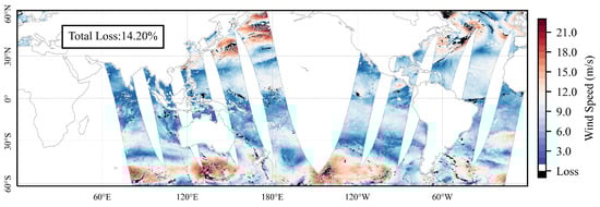
Figure 1.
The observation results of HY-2B HSCAT on 7 March 2019 indicated regions of data loss marked in black, with a loss rate exceeding 14.20%.
To address the challenge of data loss, traditional spatiotemporal interpolation methods [10,11], such as Kriging [12], Bicubic [13], and Lanczos [14], rely on simplified linear or nonlinear models. Consequently, they often fail to capture complex wind field patterns. In recent years, deep learning techniques have emerged as a powerful alternative, offering the ability to handle the nonlinearity and complexity of wind field distributions. Despite this progress, significant challenges remain in applying deep learning to SSVW inpainting.
Deep learning research in SSVW inpainting is still in its early stages [15,16,17], with limited availability of high-quality datasets. Lu et al. [18] developed the R-S dataset by matching SMAP and ECMWF ERA5 data point-to-point for 78 tropical cyclones. However, this dataset lacks critical wind structure information, which is essential for accurately inpainting SSVW. Additionally, its reliance on non-real-time reanalysis data limits its broader applicability. Similarly, Hadjipetrou et al. [19] constructed a dataset based on UERRA-HARMONIE and Sentinel-1 SAR, which suffers from similar limitations. Unfortunately, neither of these datasets nor their quality control schemes are publicly available. This lack of availability significantly hinders the development of deep learning methods for SSVW inpainting tasks.
Deep learning-based inpainting models for SSVW are scarce, especially those optimized for low-resource environments. Notably, the image restoration and inpainting tasks [20,21,22] in the Computer Vision (CV) community share considerable similarities with SSVW inpainting, offering valuable technical references. These methods provide insights for developing effective models tailored to SSVW inpainting. Consequently, image restoration and inpainting models can serve as benchmark models for SSVW inpainting tasks [23]. However, most state-of-the-art (SOTA) models are primarily based on the Transformer architecture [24], such as SwinIR [25], Uformer [26], and Restormer [27], which present several challenges for SSVW inpainting. ① Physical limitations: Transformers emphasize global dependencies and dynamic adjustments between inputs through self-attention mechanisms. While effective for many tasks, this approach is less suitable for wind fields, which exhibit continuity and inherent interdependencies in the observed medium [28]. ② Computational complexity: Transformer models typically exhibit quadratic growth in computational complexity with increasing input resolution [29]. This creates a significant computational burden for SSVW inpainting, where processing large spatial wind fields is often required. The high computational demands of Transformer-based models hinder their deployment on resource-constrained devices [30]. Thus, there is an urgent need to develop a more physically meaningful, efficient, and lightweight deep learning framework for SSVW inpainting tasks.
To address these challenges, (1) we first construct a publicly available benchmark dataset for SSVW, named SSVW Inpainting Dataset (WID), tailored for deep learning methods. WID comprises 123,841 SSVW samples collected from HY-2B HSCAT observations. Its main features include: ① Comprehensive coverage of all TC cases observed from October 2018 to April 2022. ② High-wind samples with a resolution of 25 km × 25 km and dimensions of 32 × 32, where each sample contains at least one wind speed value exceeding 17.2 m/s. ③ A diverse range of data loss scenarios, with missing data rates reaching up to 80%. (2) Secondly, we propose an effective inpainting model for SSVW, called Wind-Mamba (WMamba), which optimizes inpainting accuracy while maintaining low computational overhead. The core of WMamba is the Attention-Structured State Space Duality (ASSD), designed to capture strong interrelations and dependencies across the wind field. By employing a fluid dynamics-inspired continuous model, ASSD enables long-range semantic modeling with linear computational complexity, significantly enhancing inpainting accuracy. To address the local pixel degradation issues inherent in the original Structured State Space Duality (SSD) framework, we develop the Grouped Multi-Scale Attention Block (GMAB). The WMamba model is constructed by stacking multiple ASSD modules within a Residual-in-Residual Dense (RRD) architecture. Extensive experiments demonstrate that WMamba outperforms existing baselines, establishing itself as a robust and effective backbone for SSVW inpainting. (3) Additionally, we introduce a lightweight variant, L-WMamba, designed for deployment on resource-constrained devices. Despite its reduced complexity, L-WMamba achieves performance comparable to WMamba. The source code is available at https://github.com/njushixinjie/WMamba (accessed on 2 October 2025).
Our contributions are summarized as follows:
- (1)
- A high-quality deep learning benchmark dataset is presented for SSVW inpainting tasks.
- (2)
- We innovatively introduce and improve the SSD architecture (ASSD), designing WMamba, which achieves high-accuracy SSVW inpainting with extremely low computational resource requirements. Additionally, the GMAB module is designed to enhance the model’s performance.
- (3)
- Experiments demonstrate that WMamba outperforms other SOTA models, establishing it as a powerful and promising backbone network for SSVW inpainting.
- (4)
- We present a lightweight inpainting model, L-WMamba, which enhances deployment capabilities on resource-constrained devices while maintaining competitive performance.
2. Related Work
2.1. State Space Model (SSM)
The state space model (SSM) is rooted in classical control theory, with the structured state-space sequence model (S4) [31], which represents a novel type of sequence model in the realm of deep learning. S4 efficiently manages sequential data with linear or near-linear complexity. It can adeptly capture long-term dependencies inherent in certain data modalities. SSM can be conceptualized as a hybrid of recurrent neural networks (RNNs) and convolutional neural networks (CNNs). They draw inspiration from classical state-space model systems, which utilize implicit latent states to map one-dimensional sequences .
The integration of Equation (1) into a practical deep learning algorithm is typically achieved through discretization. Specifically, let denote the time scale parameter, which transforms the “continuous parameters” into “discrete parameters” . A commonly used discretization method is known as the zero-order hold (ZOH) rule [32], defined as follows:
After transforming , the model can be computed in two ways: either as a linear recurrence (3) or as a global convolution (4). This enables the utilization of convolution properties for parallel training. Inference can benefit from the complexity inherent in RNNs (where n represents the sequence length).
where , , . k represents the length of the input sequence, ∗ signifies the convolution operation, and K denotes a structured convolution kernel.
Mamba [28,33] is characterized as a selective state space model (S6), utilizing hardware-aware algorithms. Its primary innovation lies in the Selective Scan operation. In Mamba, , B, and C in Equations (1) and (2) become functions of the input. This reparameterization allows the model to indefinitely retain essential and relevant data, thereby enhancing the long-range linear time series modeling capabilities of SSMs. In IR tasks informed by the Mamba architecture, MambaIR [29] further resolves the balance between global perception range and computational efficiency encountered by existing methods. At similar computational costs, MambaIR outperforms the Transformer-based baseline model SwinIR.
2.2. Structured State Space Duality (SSD)
To further enhance the capabilities of Mamba, the SSD algorithm [34] utilizes the block decomposition of semi-separable matrices, leveraging the storage hierarchy provided by GPUs to achieve optimal trade-offs across various efficiency axes (such as training and inference computation, memory usage, etc.). Specifically, the SSD layer modifies the original formulation: it reduces the diagonal matrix A (referred to as the matrix or High-Order Polynomial Projection Operator) in Equation (3) to a scalar, and it expands the state space dimension from 16 to 256, thus enhancing both model performance and training/inference efficiency. By drawing upon the multi-head attention mechanism, a multi-input SSM (SSD) is created. Furthermore, by establishing a connection with attention mechanisms, SSD can seamlessly integrate optimization techniques amassed by Transformer architectures into SSMs. The training speed of the SSD model surpasses that of Mamba’s parallel associative scanning by a factor of 2 to 8. It maintains performance comparable to that of Transformers. Collectively, these advancements in state space modeling aim to enhance the efficiency and performance of sequential data processing in various applications [35].
3. WID: SSVW Inpainting Dataset
3.1. Data Collection and Quality Control
The HY-2B satellite, launched on 25 October 2018, is China’s first operational ocean dynamic environment satellite. It is equipped with a Ku-band microwave scatterometer (HSCAT-B), primarily designed for global SSVW measurements. The HSCAT achieves a global ocean coverage of at least 90% within 1 to 2 days. The HY-2B satellite ground data processing system is developed and operated by the National Satellite Ocean Application Service (NSOAS).
The data used in this study originate from the HY-2B HSCAT Level 2B (L2B) wind product and covers the period from October 2018 to April 2022. These products are retrieved using the Pencil-beam Wind Processor (PWP) method and the NSCAT-4 geophysical model function, providing 25 km × 25 km along-track gridded wind data. The data are publicly accessible at https://osdds.nsoas.org.cn/OceanDynamics (accessed on 2 October 2025).
In the HY-2B L2B dataset, the wvc_quality_flag serves as the quality indicator for wind vector cells. A wind vector cell is classified as corrupted or lost if it meets any of the following criteria:
- ①
- The wind vector cell is determined to be affected by heavy rainfall during the wind vector retrieval process, or the signal-to-noise ratio of the beam exceeds the threshold.
- ②
- Anomalies are detected in wind field variability, or product monitoring is unavailable.
- ③
- There are insufficient high-quality backscatter coefficient measurements for wind field retrieval, or the wind vector retrieval process fails.
For regions with missing SSVW data, we use data from the fifth-generation global atmospheric reanalysis dataset (ERA5), provided by the European Centre for Medium-Range Weather Forecasts (ECMWF), as a substitute. The ERA5 data is considered the ground truth and can be freely downloaded via the Copernicus Climate Change Service (C3S) platform at https://cds.climate.copernicus.eu (accessed on 2 October 2025). ERA5 supports applications in various fields, including climate trend analysis, extreme event studies, renewable energy assessments, and marine meteorology.
3.2. Dataset Construction and Statistics
To maintain consistency with the deep learning experimental framework, all wind samples are formatted as square-shaped images. Additionally, to facilitate the analysis of high-wind regions of interest in this study, we ensure that each wind sample can capture the primary impact area of a tropical cyclone or typhoon. Given that the typical diameter of typhoons ranges from 400 to 600 km, occasionally extending to 800 to 1000 km [36], the coverage of a single experimental sample is set to 800 km × 800 km, corresponding to a 32 × 32 sample size. Furthermore, the sampling stride is set to 16, which is smaller than the sampling length, to mitigate the impact of resampling on wind field continuity.
3.2.1. Wind Speed Distribution and Data Loss Situations
This study primarily focuses on inpainting techniques for high-wind data. To maximize the inclusion of high-wind samples, we establish two control conditions during the sampling process. ① Within a single day of HY-2B observations, there must be at least one clear and complete typhoon case. ② Each SSVW sample (32 × 32) must contain at least one observation point with a wind speed value of ≥17.2 m/s. This establishes a solid foundational dataset for analyzing the model’s performance across different wind speed ranges. Our dataset is specifically designed for high-wind scenarios where HY-2B HSCAT data loss is most severe due to rain contamination. Operational deployment for mixed wind regimes should require fine-tuning on representative low-wind samples or domain adaptation techniques.
Additionally, we conduct a statistical analysis of the data loss ratio in the dataset samples, which is defined as the proportion of lost pixels to the total number of pixels within the observational range of a single sample. The data loss ratio in the dataset ranges from 0 to 80%. We set the data loss ratio intervals in increments of 10%. The proportions of samples within the data loss ratio intervals (0, 10], (10, 20], (20, 30], (30, 40], (40, 50], and (50, 80] are 65.6%, 22.2%, 8.0%, 2.6%, 1.0%, and 0.6%, respectively.
3.2.2. Dataset Composition
Based on the aforementioned quality control criteria, we initially acquired 123,841 samples. The samples comprise four variables: U-component (Eastward Wind), V-component (Northward Wind), Wind Speed, and Wind Direction. These samples are divided into training and test sets at a ratio of 0.85:0.15. The test set includes all samples from multiple observation days across the globe, allowing for the reconstruction of inpainting results to demonstrate the performance on a global scale. We have named this dataset WID (SSVW Inpainting Dataset), which is publicly accessible via the following link: https://zenodo.org/records/16945879 (accessed on 10 January 2026).
4. Methodology
4.1. Overall Architecture
As illustrated in the left panel of Figure 2, WMamba consists of three stages: ① Shallow Feature Extraction (SFE), which is shown in Figure 2a, ② Deep Feature Extraction (RRD-ASSD), which is shown in Figure 2b, and ③ High-Quality Reconstruction (REC), which is shown in Figure 2c. For a wind sample (Winds Loss) requiring inpainting, denoted ∈, the first step involves employing an SFE module. This module comprises a depthwise convolutional layer and standard convolutional layers to extract shallow features, denoted by . Next, is fed into the RRD-ASSD module to obtain the deep features, . The RRD-ASSD consists of six densely connected ASSDs, which are organized in a Residual-in-Residual architecture. The residual connection branches are designed as Squeeze-Excitation Blocks (SEBs). The SEB, illustrated in Figure 2d, enhances feature representation through both channel compression and restoration. Finally, is processed via a REC module composed of multiple convolutional layers. This step generates the reconstructed wind field, denoted as .
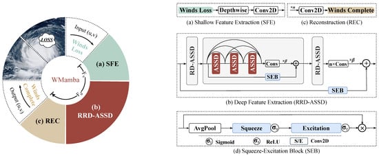
Figure 2.
The overall network architecture of our WMamba, as well as the (a) Shallow Feature Extraction (SFE) module, the (b) Deep Feature Extraction (RRD-ASSD) module, the (c) Reconstruction (REC) module and the (d) Squeeze-Excitation Blocks (SEB).
4.2. RRD-ASSD
To execute deep feature extraction efficiently with fewer network parameters, the RRD-ASSD module is constructed on the Residual-in-Residual Dense (RRD) architecture. The RRD structure incorporates residual blocks and dense connection blocks. Residual connections enhance the network’s capacity for learning details at various levels, while dense connections augment feature propagation and reuse, thereby improving the overall expressive capability of the features. Due to the effective reuse of feature maps, high-performance results may be attained through a decrease in the number of network parameters.
As shown in Figure 2b, six ASSD modules are densely connected, ensuring accurate feature representation. Next, an additional convolutional layer is integrated to refine the extracted features. Subsequently, the features are scaled by a factor and added to the corresponding residual connection branch, forming the RD-ASSD. By concatenating the RD-ASSD module four times and assigning the scaling factor once again, it is further incorporated into the residual connection branch, leading to the final configuration of the RRD-ASSD.
It is important to note that not all residual connections in the RRD-ASSD directly contribute to the module’s output. Rather, they are subjected to an attention mechanism known as the Squeeze-Excitation Blocks (SEBs). The SEB calculates channel attention weights to adjust the significance of each channel in the input feature map. Specifically, as illustrated in Figure 2d, the SEB module comprises global average pooling and channel scaling convolution layers, along with and activation functions.
4.3. ASSD: Attention-Structured State Space Duality
As a critical component of the WMamba model, the Attention-Structured State Space Duality (ASSD) module is illustrated in Figure 3a. It consists of the SE-SSD Block and the Grouped Multiscale Attention Block (GMAB), configured sequentially. Furthermore, we introduce learnable coefficient factors and . These factors facilitate residual connections for the two modules. Layer Normalization is applied before each sub-module to stabilize the training process.
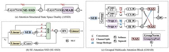
Figure 3.
Architecture diagram of (a) Attention-Structured State Space Duality (ASSD), which consists of two important components: (b) SE-Attention SSD (SE-SSD) and (c) Grouped Multiscale Attention Block (GMAB).
4.3.1. SE-SSD: SE-Attention SSD
As shown in Figure 3b, the SE-SSD incorporates the SSD for long-distance feature modeling with linear complexity. Initially, the input feature of the SE-SSD module is processed through two linear mapping branches. This results in the features and . In the first branch, is fed into the SEB and further into the SSD module. Subsequently, using a multi-head attention mechanism, the feature , which has been enhanced through the SEB and activated via the activation function , is also fed into the SSD layer. In the second branch, is processed through a simple convolutional layer followed by the . It is then multiplied by the output Y of the SSD. Ultimately, after passing through a Batch Normalization layer and a linear mapping layer, we obtain the output feature of the SE-SSD. The state space dimension of SE-SSD is extended to 128.
4.3.2. GMAB: Grouped Multiscale Attention Block
As previously described, the GMAB module is designed to counter local pixel degradation by jointly exploiting global context and fine-grained spatial details. Using grouped operations and multiscale convolutions, it first amplifies the input features via the SEB layer (Figure 3c). These enriched features are then partitioned into two independent groups to reduce computational overhead and parameter count.
Group-1 performs adaptive, multiscale pooling along the height and width dimensions ( and ), thereby extracting global spatial representations. Group-2 employs cascaded, multilayer convolutions that capture local features across heterogeneous receptive fields. Both groups concurrently execute a Separation–Activation–Fusion operation, in which residual connections are integrated with the grouped features to further refine the representation.
Subsequently, the NAS (Norm-AvgPool-Softmax) module computes cross-group attention weights that selectively reweight the feature maps, ensuring that salient patterns are emphasized while irrelevant cues are suppressed. Finally, the group-wise outputs are aggregated and re-integrated with the original grouped features through residual connections, endowing the model with enhanced representational capacity.
4.4. L-WMamba: Light-WMamba
In addition, based on the WMamba architecture, the number of convolutional layers in the REC module is reduced to one-third of the original. Both the number of ASSD modules and that of the cascaded RRD-ASSD modules are halved. The dimensions of Input Channels (: 128 to 64), State Dimensions (: 128 to 64), and Head Dimensions (: 64 to 8) in ASSD are reduced, resulting in a lighter version of WMamba called L-WMamba.
4.5. Adaptive Weighted Loss Function
Given that our research primarily focuses on SSVW inpainting under high-wind conditions, which are often accompanied by higher data loss ratios, we introduce an adaptive weighting factor, , into the L2 Loss Function (MSE). This factor automatically assigns greater loss weights to samples with a loss ratio exceeding 10%. The calculation formula for is shown below:
In addition, we create sample masks where loss regions are marked as 1 and non-loss regions are marked as 0. The loss function computes the error only within the loss regions. The overall loss function can be expressed as follows:
where N is the total number of samples, represents the output of winds, and signifies the ground truth winds.
4.6. Evaluation Metrics
The performance of the inpainting model is thoroughly evaluated from three key perspectives: pixel-level discrepancy (RMSE and Bias), fidelity of spatial structure (MS-SSIM), and fidelity of the frequency domain (RAPSD).
4.6.1. RMSE and Bias
First, the RMSE is adopted to quantify the pixel-wise deviation between the model predictions x and the ground-truth observations y, expressed as:
where N denotes the total number of spatial pixels. Subsequently, the systematic is introduced to characterize the directional discrepancy (over- or underestimation) in winds inpainting.
4.6.2. MS-SSIM
Additionally, the Structural Similarity Index Measure (SSIM) quantifies image perceptual quality by jointly assessing luminance, contrast, and structural similarity between two images [37]. Unlike pixel-wise metrics, SSIM emphasizes structural coherence. Nevertheless, its single-scale formulation can overlook fine-scale details in multi-scale phenomena such as SSVW. Specifically, SSIM may fail to capture local wind-field gradients and mesoscale vortices, thereby limiting its diagnostic power. The formula for SSIM is as follows:
where and are the means, and are the variances, and is the covariance, respectively. and are included to ensure numerical stability. L denotes the dynamic range of the wind speed values, which is the maximum wind speed value of 32.74 m/s in the WID dataset. The values of and are set to 0.01 and 0.03, respectively.
To address this limitation, we adopt Multi-Scale SSIM (MS-SSIM), an extension that evaluates similarity across multiple spatial resolutions [38]. MS-SSIM is computed as follows: first, an image pyramid is constructed by successively downsampling the reference x and reconstructed y images via Gaussian filtering and subsampling, yielding M scale levels. Second, the SSIM value at the i-th scale, , is calculated. Finally, the values are weighted by and aggregated:
4.6.3. RAPSD
Frequency-domain analysis of wind field data offers a direct view of its spectral energy distribution, which is essential for diagnosing a model’s ability to resolve small-scale atmospheric structures. To this end, we employ Radial Average Power Spectral Density (RAPSD), a diagnostic that compresses two-dimensional spectral information into a one-dimensional radial average. Let the SSVW image be denoted by , and let its two-dimensional Fourier transform be , where x and y represent the horizontal and vertical wavenumber components, respectively. The Power Spectral Density (PSD) is then given by
The radial wavenumber k is defined as . . Aggregating the PSD over all spectral points enclosed within the annulus , the RAPSD is expressed as
where denotes the number of discrete wavenumbers within the specified radial interval.
5. Experimental Results and Analyses
As previously noted, image restoration and inpainting methods serve as reliable baselines for SSVW inpainting tasks. We compare WMamba against seven SOTA models: SwinIR (ICCV2021), UFormer (CVPR2022), Restormer (CVPR2022), FocalNet (NeurIPS2022) [39], GRL (CVPR2023) [40], AST (CVPR2024) [41], and MambaIR (ECCV2024).
For comparative analysis, we benchmark our approach against three widely adopted interpolation techniques: Bicubic, Kriging, and Lanczos. Bicubic ensures local continuity with minimal computational overhead, making it suitable for real-time or large-scale gridded resampling. Kriging leverages a semi-variogram to yield the spatial best-linear-unbiased estimate and simultaneously delivers a predictive variance, thereby furnishing a rigorous confidence measure. Lanczos interpolation employs a Lanczos-windowed sinc kernel, markedly preserving texture and edge acuity.
5.1. Overall Analysis
The quantitative analysis considers wind speed (including U and V components) and wind direction. It is important to note that the RMSE and Bias metrics are calculated only for the loss regions, while MS-SSIM and RAPSD are computed across the entire sample area. Additionally, due to the periodic nature of wind direction, its deviation may result in two distinct values (clockwise and counterclockwise). In this study, the deviation with the smaller absolute value is consistently selected. Finally, when calculating the Bias value, deviations in the clockwise direction are defined as positive, whereas those in the counterclockwise direction are defined as negative.
5.1.1. RMSE, MS-SSIM and Bias
Table 1 presents a quantitative comparison of WMamba with other methods in terms of wind speed (including U and V components) and wind direction. WMamba demonstrates superior performance across nearly all evaluation metrics. Specifically, WMamba achieves RMSE values of 0.9636 m/s for wind speed and 14.5319° for wind direction, with MS-SSIM scores of 0.9931 and 0.9906, respectively. Additionally, the Bias values for WMamba are very close to zero. The second-best model is GRL. Compared to GRL, WMamba reduces the RMSE of wind speed by 11.41% and the RMSE for wind direction by 6.26%, representing a significant improvement over the previous SOTA model.

Table 1.
Quantitative comparison of the WMamba with various deep-learning and interpolation methods. The analysis focused on two aspects: wind speed (including U and V components) and wind direction. Three metrics are used for evaluation: RMSE, MS-SSIM, and Bias. The best, the second best, and the third best results are denoted as ★bold, underlined, and *italicized, respectively.
Furthermore, we analyze the performance of three interpolation methods. Overall, the interpolation methods perform significantly worse than deep learning-based approaches. Among the interpolation methods, Kriging yields the best results, achieving an RMSE of 2.9239 m/s for wind speed and 24.2563° for wind direction. Compared to Kriging, WMamba reduces the RMSE of wind speed and wind direction by 67.04% and 40.09%, respectively. Notably, the Bias values for wind speed in all interpolation methods are lower than −1.04 m/s, indicating that these methods tend to underestimate wind speed overall.
Lastly, we analyze the performance of L-WMamba in detail. For wind speed, the performance of L-WMamba relative to RMSE corresponds to 86.34%, 97.46%, and 97.99% of WMamba (ranked first), GRL (ranked second), and Restormer (ranked third), respectively. For wind direction, the RMSE of L-WMamba achieved 92.33% and 98.49% of the performances of WMamba and GRL, respectively, and even surpassed that of Restormer (ranked third). These results demonstrate that L-WMamba achieves performance competitive with the best models.
5.1.2. Frequency Domain Analysis: RAPSD
WMamba exhibits outstanding performance in the spatial domain. Next, we conduct a frequency domain analysis. During the RAPSD computation, the radius is divided into 10 bins, ranging from 1 to 10, with frequency gradually increasing. As shown in Figure 4a, we calculate the average power spectral density across different radial frequency intervals. To facilitate comparison, the logarithm of RAPSD is utilized. Overall, all methods underestimate the wind field’s energy density across every frequency range. Notably, WMamba (red line) exhibits a trend closest to the Ground Truth (black line).
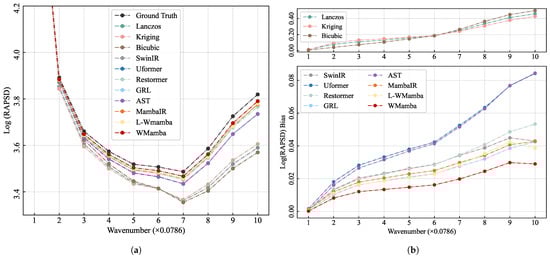
Figure 4.
The Radial Average Power Spectral Density (RAPSD) results for different methods are presented. (a) The logarithmic values of RAPSD at different wavenumbers, (b) the bias of the Log(RAPSD) values of different methods from the ground truth. The radial frequency radius is divided into 10 groups, with higher wavenumbers representing higher frequencies.
As shown in Figure 4b, we further present a comparative analysis of the differences between various methods and the Ground Truth. Due to the significant performance differences between the three interpolation methods and other deep learning approaches, we display their performance on two separate subplots for clarity. Among all methods compared, WMamba shows the lowest deviation values across all frequency radii, indicating that WMamba performs well in capturing the overall energy distribution of the SSVW. WMamba effectively approximates the true SSVW across different scales, showcasing strong multi-scale adaptability, particularly in the high-frequency region (i.e., larger wavenumbers). It not only preserves the overall structure of the SSVW but also effectively recovers fine details.
Consistent with the spatial domain metrics, the three interpolation methods (Lanczos, Kriging, and Bicubic) continue to exhibit significant disparities compared to deep learning-based methods. This discrepancy becomes increasingly pronounced in the high-frequency range, suggesting that interpolation results are overly smoothed, leading to a substantial loss of detailed information. Notably, Kriging demonstrates better high-frequency detail reconstruction, although its performance in the low-frequency range is slightly weaker. This phenomenon is the exact opposite of what is observed with the Bicubic method. Additionally, GRL ranks second in the frequency domain, while MambaIR outperforms Restormer. As a model also based on the Mamba framework, MambaIR demonstrates outstanding performance in detail restoration. Importantly, L-WMamba achieves the second-best performance, surpassing GRL in the mid-to-low frequency range. However, due to the absence of the GMAB module, its performance slightly degrades in the high-frequency range.
5.2. Model Complexity Comparison
In evaluating model complexity, it is essential to consider both the number of parameters () and Floating Point Operations (). When assessing the demands on computational resources, serves as a more direct metric, as it directly correlates with the model’s computational complexity and operational efficiency. However, the number of parameters should not be overlooked, particularly in resource-constrained environments such as devices or embedded systems, where storage and memory requirements are also critical.
refers to the total count of trainable weights and biases within the model. Models with a higher number of parameters typically exhibit greater capacity and demand more memory for storage. As shown in Table 2, WMamba has the lowest parameter count at just 1.06 M among all base models. Remarkably, WMamba also achieves the best performance. In contrast, the parameter counts of other models are several to dozens of times greater than that of WMamba.
Table 2.
Complexity comparison of deep learning models, in which is measured in M and in G.
Additionally, quantifies the number of floating-point operations executed during a single forward pass of the model. Models with higher require more robust computational resources (for instance, GPUs). As depicted in Table 2, WMamba exhibits the third-lowest count at 2.15 G, indicating a minimal demand for computational resources (GPUs). This suggests that WMamba is capable of operating on edge GPU platforms with limited capabilities.
To enhance the applicability of our model on GPU platforms with limited memory, we developed L-WMamba, which also demonstrates the scalability of our approach. The parameter count of L-WMamba (0.36 M) is only one-third that of our base model (WMamba), and its (0.54 G) is merely one-fourth of WMamba. It is noteworthy that the performance of L-WMamba closely approximates that of the top three models, substantiating the scalability and efficiency of this approach.
5.3. Visual Comparison
To demonstrate the method’s generalizability, we include examples spanning the entire global ocean. Figure 5a–d present the HY-2B observations from 6 September 2021 (with black regions indicating loss data), the WMamba inpainting results, the Ground Truth, and the difference between WMamba and the Ground Truth. In Figure 5a, the magnified subplots illustrate the precipitation distribution during Hurricane LARRY’s passage (provided by ERA5) and the corresponding data loss. It is evident that the regions of intense precipitation closely align with the high-wind zones of the hurricane, which are also the primary areas of data loss. This finding intuitively demonstrates how precipitation impacts Ku-band data acquisition. As shown in Figure 5b, WMamba effectively reconstructs all loss regions, and visually, the results are highly consistent with the Ground Truth (Figure 5d).
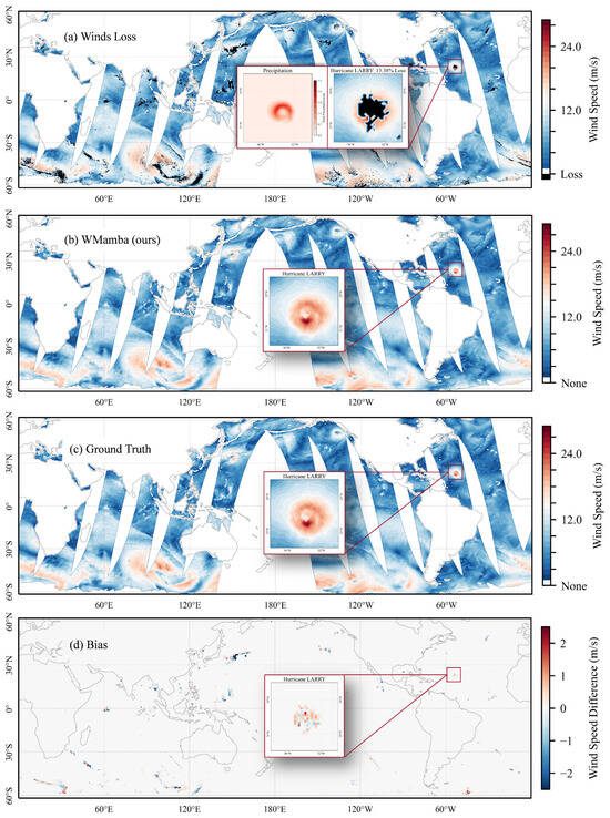
Figure 5.
The data from 6 September 2021, including (a) HY-2B observations (with black regions representing loss data), (b) WMamba inpainting results, (c) the Ground Truth, and (d) the differences between WMamba and the Ground Truth. The magnified inset highlights Hurricane LARRY’s primary impact area at 21:50. In panel (a), the accompanying precipitation distribution during LARRY’s passage, provided by ERA5, is also displayed.
It is worth noting that while WMamba achieves near-zero global bias (−0.0204 m/s), this metric masks significant spatially coherent errors in high-gradient regions. As shown in Figure 5d, systematic bias patterns emerge around tropical cyclone centers, with wind speed overestimation in outer quadrants and underestimation near the eye-wall interface. This dipole-like structure reflects the model’s difficulty in resolving sharp intensity gradients and precise eye-wall positioning, rather than random prediction noise. The global bias cancellation results from opposing errors in different storm sectors, not uniform accuracy. This limitation is inherent to the training data: ERA5’s smoothed fields lack fine-scale eye-wall sharpness, and the MSE loss optimizes for mean accuracy rather than extreme-gradient fidelity. Users should interpret global metrics cautiously, prioritizing spatial structure metrics (MS-SSIM, RAPSD) for high-wind validation.
To better examine the details of the inpainting, we conduct a visual analysis of two HY-2B observations of Hurricane LARRY on the same day. These observations are taken at 9:40 (Region-1) and 21:50 (Region-2). WMamba is compared to three representative models: GRL (ranked second overall and the best-performing Transformer-based architecture), MambaIR (based on the Mamba framework), and Kriging (the best-performing interpolation-based method).
5.3.1. Region-1 at 09:40
Figure 6I shows Region-1, with its center located at 52°W and 18°N. Hurricane LARRY passed through this region on 6 September 2021 at 9:40. Region-1 has a loss data ratio of 6.40%. Visually, the inpainting results of WMamba, GRL, and MambaIR closely resemble the Ground Truth, accurately depicting the structure of the hurricane’s center. Notably, WMamba demonstrates the most precise wind direction reconstruction in the hurricane’s center, validating its strong ability to restore local details. In contrast, the Kriging method displaces the hurricane’s center and significantly overestimates the area of low-wind regions near the center, severely underestimating the wind speed in the hurricane’s core. To further analyze the discrepancies, we calculate the difference between the inpainting results of each model and the Ground Truth, as shown in the second line of Figure 6I. WMamba outperforms other models in both wind speed and wind direction accuracy, indicating its superior capability in reconstructing the detailed structure of the hurricane’s center. However, it is worth noting that both WMamba and MambaIR slightly underestimate the hurricane’s wind speed, while GRL exhibits the opposite trend.
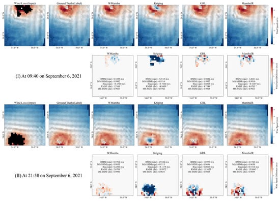
Figure 6.
The observations of Hurricane LARRY on 6 September 2021 from the ascending (I) and descending (II) orbits of HY-2B are presented. In each subplot, the first row shows the inpainting results (wind speed and wind direction) from different models, while the second row displays the difference maps compared to the ground truth.
5.3.2. Region-2 at 21:50
For Hurricane LARRY, HY-2B HSCAT conducted a second observation on the same day at 21:50. As illustrated in Figure 6II, the loss data ratio in this area is as high as 9.69%, primarily concentrated in the hurricane’s central structure. This significantly impacts the analysis of the wind field structure. Similar to Region-1, WMamba’s reconstruction in Region-2 is visually the closest to the Ground Truth, accurately capturing the hurricane’s center location while maintaining an evident advantage in wind direction accuracy. It is worth noting that, aside from the Kriging method, MambaIR also displaces the hurricane’s center. The second line of Figure 6II displays the inpainting deviations of different models in Region-2. WMamba achieves wind speed and wind direction RMSEs of just 0.5768 m/s and 2.6709°, respectively, while the second-ranked GRL exhibited significantly higher RMSEs of 1.8977 m/s and 11.3625°. These quantitative results further support the visual analysis.
5.4. Performance of the Models in Different Loss Ratios
The inpainting performance under different loss ratios is a critical criterion for evaluating model stability. As shown in Figure 7a,b, in terms of both wind speed and wind direction, WMamba consistently outperforms other methods across all loss ratio intervals, achieving the lowest RMSE values.
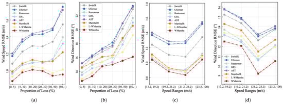
Figure 7.
The RMSE of wind speed and wind direction for representative inpainting models under different loss data ratios (a,b), as well as the RMSE of wind speed and wind direction across different wind speed ranges (c,d), are presented.
Our dataset covers loss ratios ranging from 0% to 80%. Generally, samples with higher loss ratios are more difficult to reconstruct, leading to larger inpainting errors. Figure 7a,b confirm this pattern. As the loss ratio increases, the RMSE values of most models exhibit a steady upward trend.
As discussed earlier, to ensure the model pays more attention to samples with higher loss ratios, we assigned greater incentive weights to these samples. As shown in Figure 7a, when the loss ratio exceeds 10%, WMamba demonstrates an increasing advantage over the second-best model, GRL. This indicates that WMamba has a more significant inpainting accuracy advantage under high loss ratios. Such an advantage enhances WMamba’s robustness in handling observations with large-scale data loss.
5.5. Performance of the Models in Different Wind Speed Ranges
Using the maximum wind speed of each sample as the classification criterion, we categorize all samples into four distinct wind speed ranges, starting from 17.2 m/s and incrementing by 2 m/s for each class.
The performance of the WMamba model is comprehensively evaluated across various wind speed ranges against other SOTA models. The analysis of RMSE for wind speed and wind direction (Figure 7c,d) indicates that WMamba consistently outperforms other baseline models across all speed ranges. Its superiority is particularly evident in the higher wind speed intervals of [21.2, 23.2] m/s and [23.2, 100] m/s, demonstrating WMamba’s remarkable capability in accurately inpainting SSVW under high-wind conditions.
5.6. Ablation Study
Our study innovatively introduces the SSD architecture into the SSVW inpainting. Additionally, we develop the GMAB module to address the inherent local information loss issue associated with SSD. To verify the effectiveness of GMAB, we establish another baseline model, w/o GMAB, which excludes the GMAB module from WMamba. Furthermore, we include L-WMamba in the comparative experiments.
As shown in Table 3, the removal of GMAB increases the RMSE of wind speed by 9.49% and wind direction by 6.04% while also causing a noticeable reduction in MS-SSIM. This demonstrates the significant contribution of GMAB to improving overall accuracy. The wind speed field exhibits pronounced multi-scale spatial heterogeneity, characterized by steep gradients within the typhoon eye-wall and smooth transitions in the outer regions. The multi-scale convolution branch (Group-2) of GMAB is better suited to capturing such features. In contrast, wind direction, as a vectorial angular variable, is governed predominantly by large-scale circulation patterns, where global contextual information (adaptive pooling in Group-1) contributes more substantially, resulting in lower sensitivity to local detail enhancement.
Table 3.
Ablation experiment of WMamba, L-WMamba and GMAB module.
To specifically validate the attention mechanism within SSD (distinct from GMAB’s multi-scale role), we test a variant replacing SE-SSD with standard Mamba blocks. This increased wind speed RMSE by 4.10% (to 1.0031 m/s) and direction RMSE by 2.98% (to 14.9650°), confirming that attention-structured state transitions are critical for adaptive wind field modeling, not merely architectural embellishment.
Although the lightweight version reduces the overall accuracy, it significantly decreases the model’s parameter count and , improving the feasibility of deploying WMamba on resource-constrained mobile platforms.
6. Discussion
6.1. Physical Motivation for SSD in Wind Fields
The SSD framework is well-suited for SSVW modeling due to its ability to capture spatiotemporal dependencies in a continuous medium [34]. Unlike particle-based methods or Transformer’s pairwise token attention, SSD leverages the Lie exponential map to encode both global and local dependencies [42], mirroring how momentum diffuses in fluid systems. Specifically, the linear recurrence in Equation (3) extends continuum mechanics by incorporating state evolution over time: the hidden state accumulates past information through , analogous to how atmospheric memory persists in boundary layer processes. While fluid systems lack strict memory, SSD’s structured state transitions approximate evolving wind patterns more naturally than Transformer’s position-agnostic attention, which ignores the directional, causal propagation of geophysical flows. This makes SSD particularly effective for capturing turbulence, stratification, and dynamic variability in SSVW data.
6.2. Limitations of ERA5 as Auxiliary Data
We acknowledge that ERA5 reanalysis data has documented limitations in representing extreme wind speeds, particularly in tropical cyclone cores where its coarse resolution (28 km) and assimilation smoothing can significantly underestimate peak winds exceeding 20 m/s [43]. In our framework, ERA5 serves solely to provide physically plausible constraints for missing regions in HY-2B HSCAT observations, while the model primarily learns from available HSCAT measurements to preserve Ku-band scatterometer characteristics. Consequently, WMamba reconstructs wind fields that are consistent with HSCAT’s statistical distribution rather than replicating ERA5’s smoothed patterns, as validated by spectral fidelity metrics (Figure 4) and spatial consistency checks (Figure 6). Users should interpret the inpainted results as HSCAT-compatible reconstructions, recognizing that absolute peak wind speeds in extreme events may retain ERA5’s inherent smoothing bias.
6.3. Deployment and Efficiency of the L-WMamba
In-depth analysis of real-world deployment performance further underscores the advantages of our lightweight model, L-WMamba.
6.3.1. Storage and Memory Overhead
As shown in Table 4, L-WMamba requires just 0.36 M parameters—over 140× fewer than Uformer-B (50.39 M)—and only 0.54 G FLOPs, just 1/18th of Restormer-B’s 2.56 G. At 0.56 MB, its Flash footprint is well below the 1 MB threshold of many end devices. Activation caches and temporary buffers scale down proportionally, substantially reducing DRAM demands and enabling deployment on low-power hardware. The sub-MB size of the model eliminates the need for external high-capacity flash storage or SSDs, making it suitable for ultra-low-power scenarios such as IoT devices and wearables.
Table 4.
Actual inference performance of each model on typical computing platforms, including model size, inference time (latency), and throughput.
6.3.2. Energy Efficiency
Fewer FLOPs translate to shorter compute cycles and lower average power consumption. On power-constrained platforms such as the Jetson Nano and ARM CPUs, L-WMamba reduces system power usage by over 40% compared to competing models.
6.3.3. Real-Time Performance
We evaluated all models across high-performance GPUs (RTX 3090), edge GPUs (Jetson Nano), and embedded ARM CPUs (INT8). On the RTX 3090, L-WMamba achieves just 0.02 ms latency and up to 50,000 FPS—far surpassing SwinIR-B (250 FPS) and Uformer-B (2000 FPS). This headroom supports higher concurrent loads or more complex post-processing in server/cloud deployments. On the Jetson Nano, L-WMamba consistently exceeds 60 FPS—2–3× the 20 FPS of AST-B and 25 FPS of Uformer-B. Even on ARM CPUs limited to INT8 precision, it delivers 25–30 FPS versus the typical 6–15 FPS of other models, satisfying real-time requirements in power- and heat-sensitive scenarios such as drones and smart sensors.
In summary, by minimizing parameters and computation (0.36 M and 0.54 G), L-WMamba achieves outstanding real-time inference across diverse hardware. Compared to current SOTA models, it not only meets but exceeds frame-rate requirements while minimizing storage, energy, and compute footprints—ideal for resource-constrained or multi-model parallel deployments. With its “high-speed, low-power, end-cloud collaborative” design, L-WMamba is especially suited to mobile, industrial embedded, and edge applications.
6.4. Future Works: Addressing the Problem of High Error Rates in Extreme Wind Speeds
In the realm of deep learning, it is widely recognized that more data leads to improved model performance. An increase in data volume exposes the model to a greater variety of samples during training. This facilitates the effective learning of complex features and patterns. Conversely, a smaller dataset risks leading to overfitting.
In the physical world, high-wind events occur significantly less frequently than low-wind events [44]. As a result, there are fewer effective samples within higher wind speed ranges. This imbalance negatively impacts the performance of the inpainting model, particularly in high-wind ranges. To tackle the imbalance issue, this study sets a high threshold for wind-speed sampling and applies synthetic data augmentation strategies.
Additionally, when applying deep learning techniques within the SSVW domain, reliance on loss functions such as Mean Squared Error (MSE) often leads to model training that reflects average characteristics (Appendix A). Specifically, the predictive errors associated with outlier samples—whether high or low—tend to be disproportionately large. Furthermore, outlier samples are inherently present. This occurs regardless of any changes made to the dataset distribution. To mitigate the issue of average characteristics, it is crucial to enhance the loss function of the neural network. By reconstructing the loss function, the attention of the neural network can be distributed more fairly across various wind speed ranges. We aim to focus our future efforts on this key research area.
7. Conclusions
This study introduces WMamba, a task-oriented deep learning framework that advances the SOTA in Sea Surface Vector Wind (SSVW) inpainting, particularly under extreme wind conditions. By addressing the 8.18–19.13% data loss rates observed in HY-2B HSCAT tracks, this work emphasizes the urgent need for robust inpainting techniques to improve meteorological forecasts and climate monitoring.
WMamba introduces the Attention-Structured State Space Duality (ASSD) architecture, which combines linear computational complexity with long-range dependency modeling. The Grouped Multi-scale Attention Block (GMAB) further mitigates local pixel degradation. While maintaining low computational overhead, WMamba achieves a wind speed inpainting accuracy of 0.9636 m/s RMSE and 0.9931 MS-SSIM, as well as a wind direction accuracy of 14.5319° RMSE and 0.9906 MS-SSIM.
To broaden deployment, we design L-WMamba, a lightweight variant that maintains competitive performance on resource-constrained devices.
Complementing the models, we release the SSVW Inpainting Dataset (WID)—a publicly available benchmark of 123,841 high-wind samples that covers all tropical cyclones from 2018 to 2022. The proportion of loss data in the samples ranges from 0% to80%.
Collectively, WMamba, L-WMamba, and WID establish a comprehensive toolkit for SSVW inpainting, paving the way for improved environmental monitoring, disaster mitigation, and broader geophysical applications.
In future work, we aim to further enhance the framework’s capabilities by integrating additional real-time datasets, such as oceanographic and atmospheric parameters, to improve inpainting accuracy. We also plan to extend the model’s applicability to other data-intensive domains, such as hydrology and disaster management, and to explore the integration of multi-modal data sources for a more comprehensive understanding of SSVW dynamics.
Author Contributions
Conceptualization, J.S., K.R. and X.S.; methodology, L.H., J.Z., Q.S. and X.S.; software, L.H., J.Z. and Q.S.; validation, L.H., J.Z. and X.S.; formal analysis, Q.S. and X.S.; investigation, L.H., J.Z. and X.S.; resources, J.S., K.R. and X.S.; data curation, L.H., J.Z. and X.S.; writing—original draft preparation, L.H., J.Z. and W.N.; writing—review and editing, L.H., W.N., Q.S. and X.S.; visualization, L.H., J.Z., Q.S. and X.S.; supervision, J.S., K.R. and X.S.; project administration, J.S., K.R. and X.S. All authors have read and agreed to the published version of the manuscript.
Funding
This research received no external funding.
Data Availability Statement
The codes are open-sourced at https://github.com/njushixinjie/WMamba (accessed on 10 January 2026). The dataset can be obtained from the following link: https://zenodo.org/records/16945879 (accessed on 10 January 2026).
Acknowledgments
We extend our sincere appreciation to the institutions that have generously provided data to support our research. Specifically, we are grateful to the National Satellite Ocean Application Service (NSOAS) for their provision of the HY-2B L2B data. Importantly, we would like to emphasize that all the data used in this study can be freely obtained from publicly available datasets. Their collaboration has been highly instrumental to the success of our work.
Conflicts of Interest
The authors declare no conflicts of interest.
Abbreviations
The following abbreviations are used in this manuscript:
| SSVW | Sea Surface Vector Winds |
| TC | Tropical Cyclones |
| HSCAT | HY-2B Scatterometer |
| WID | SSVW Inpainting Dataset |
| WMamba | Wind-Mamba |
| L-WMamba | Lightweight-WMamba |
| SOTA | State-of-the-Art |
| RMSE | Root Mean Square Error |
| MS-SSIM | Multi-Scale Structural Similarity Index Measure |
| RAPSD | Radial Average Power Spectral Density |
| Parameters | |
| Floating Point Operations | |
| SSM | State Space Model |
| S4 | Structured SSM |
| S6 | Selective SSM |
| SSD | Structured State Space Duality |
| ASSD | Attention-SSD |
| RRD | Residual-in-Residual Dense |
| RRD-ASSD | Deep Feature Extraction |
| SFE | Shallow Feature Extraction |
| SEB | Squeeze-Excitation Blocks |
| REC | High-Quality Reconstruction |
| GMAB | Grouped Multiscale Attention Block |
| NAS | Norm-AvgPool-Softmax |
| SAF | Separation–Activation–Fusion |
| BN | Batch Normalization |
| Average Pooling | |
| Convolution |
Appendix A. Details of the Implementation of Model Training
The experiments are conducted using PyTorch (v2.3.1) on NVIDIA RTX 3090 GPUs (NVIDIA Corporation, Santa Clara, CA, USA). The Adam optimizer is employed with parameters = 0.9 and = 0.999. The model is trained for 300 epochs. Furthermore, the Cosine Annealing Learning Rate (CosineAnnealingLR) scheduler is utilized. All deep learning models, including GRL, Restormer, and SwinIR, are trained from scratch on the WID dataset without leveraging pre-trained weights from ImageNet or other large-scale datasets.
The initial learning rate and batch size search spaces for training each model are as follows: [, , , …, ] and [32, 48, 64, …, 256], respectively. The optimal parameter settings for each model are shown in Table A1. It is important to note that all model metrics are obtained by averaging the results of 5 training runs under the optimal hyperparameter configurations.
Table A1.
The setting of the best hyperparameter of the models.
Table A1.
The setting of the best hyperparameter of the models.
| Methods | Learning Rate | Batch Size |
|---|---|---|
| SwinIR | 128 | |
| Uformer | 128 | |
| Restormer | 96 | |
| FocalNet | 256 | |
| GRL | 96 | |
| AST | 256 | |
| MambaIR | 64 | |
| WMamba | 32 | |
| L-WMamba | 96 | |
| w/o GMAB | 64 |
References
- Shi, X.; Su, Q.; Wang, W.; Ni, W.; Duan, B.; Ren, K. TCNet: Triple Collocation-Based Network for Ocean Surface Wind Speed Retrieval on CYGNSS. IEEE Trans. Geosci. Remote. Sens. 2024, 62, 4104814. [Google Scholar] [CrossRef]
- Shi, X.; Duan, B.; Ren, K. A More Accurate Field-to-Field Method towards the Wind Retrieval of HY-2B Scatterometer. Remote Sens. 2021, 13, 2419. [Google Scholar] [CrossRef]
- Wang, Z.; Weng, F.; Han, Y.; Hu, H.; Yang, J. Evaluations of Microwave Sounding Instruments Onboard FY-3F Satellites for Tropical Cyclone Monitoring. Remote Sens. 2024, 16, 4546. [Google Scholar] [CrossRef]
- Wang, Z.; Zou, J.; Stoffelen, A.; Lin, W.; Verhoef, A.; Li, X.; He, Y.; Zhang, Y.; Lin, M. Scatterometer sea surface wind product validation for HY-2C. IEEE J. Sel. Top. Appl. Earth Obs. Remote Sens. 2021, 14, 6156–6164. [Google Scholar] [CrossRef]
- Zhao, K.; Stoffelen, A.; Verspeek, J.; Verhoef, A.; Zhao, C. Bayesian algorithm for rain detection in Ku-band scatterometer data. IEEE Trans. Geosci. Remote Sens. 2023, 61, 4203416. [Google Scholar] [CrossRef]
- Donnelly, W.J.; Carswell, J.R.; McIntosh, R.E.; Chang, P.S.; Wilkerson, J.; Marks, F.; Black, P.G. Revised ocean backscatter models at C and Ku band under high-wind conditions. J. Geophys. Res. Ocean. 1999, 104, 11485–11497. [Google Scholar] [CrossRef]
- Fogg, B.J.; Long, D.G. An OSCAT Simultaneous Wind/Rain Geophysical Model Function. IEEE J. Sel. Top. Appl. Earth Obs. Remote Sens. 2025, 18, 17852–17864. [Google Scholar] [CrossRef]
- Shi, X.; Duan, B.; Ren, K. F2F-NN: A Field-to-Field Wind Speed Retrieval Method of Microwave Radiometer Data Based on Deep Learning. Remote Sens. 2022, 14, 3517. [Google Scholar] [CrossRef]
- Shao, W.; Lai, Z.; Nunziata, F.; Buono, A.; Jiang, X.; Zuo, J. Wind field retrieval with rain correction from dual-polarized Sentinel-1 SAR imagery collected during tropical cyclones. Remote Sens. 2022, 14, 5006. [Google Scholar] [CrossRef]
- Zeng, C.; Shen, H.; Zhang, L. Recovering missing pixels for Landsat ETM+ SLC-off imagery using multi-temporal regression analysis and a regularization method. Remote Sens. Environ. 2013, 131, 182–194. [Google Scholar] [CrossRef]
- Yin, G.; Mariethoz, G.; McCabe, M.F. Gap-filling of landsat 7 imagery using the direct sampling method. Remote Sens. 2016, 9, 12. [Google Scholar] [CrossRef]
- Oliver, M.A.; Webster, R. Kriging: A method of interpolation for geographical information systems. Int. J. Geogr. Inf. Syst. 1990, 4, 313–332. [Google Scholar] [CrossRef]
- Fan, M.; Zuo, X.; Zhou, B. Parallel computing method of commonly used interpolation algorithms for remote sensing images. IEEE J. Sel. Top. Appl. Earth Obs. Remote Sens. 2023, 17, 315–322. [Google Scholar] [CrossRef]
- Komzsik, L. The Lanczos Method: Evolution and Application; SIAM: Philadelphia, PA, USA, 2003. [Google Scholar]
- Silva, M.T.; Gill, E.W.; Huang, W. An improved estimation and gap-filling technique for sea surface wind speeds using NARX neural networks. J. Atmos. Ocean. Technol. 2018, 35, 1521–1532. [Google Scholar] [CrossRef]
- Vieira, F.; Cavalcante, G.; Campos, E.; Taveira-Pinto, F. A methodology for data gap filling in wave records using Artificial Neural Networks. Appl. Ocean Res. 2020, 98, 102109. [Google Scholar] [CrossRef]
- Lalic, B.; Stapleton, A.; Vergauwen, T.; Caluwaerts, S.; Eichelmann, E.; Roantree, M. A comparative analysis of machine learning approaches to gap filling meteorological datasets. Environ. Earth Sci. 2024, 83, 679. [Google Scholar] [CrossRef]
- Lu, J.; Ren, K.; Li, X.; Zhao, Y.; Xu, Z.; Ren, X. From reanalysis to satellite observations: Gap-filling with imbalanced learning. GeoInformatica 2022, 26, 397–428. [Google Scholar] [CrossRef]
- Hadjipetrou, S.; Mariethoz, G.; Kyriakidis, P. Gap-filling sentinel-1 offshore wind speed image time series using multiple-point geostatistical simulation and reanalysis data. Remote Sens. 2023, 15, 409. [Google Scholar] [CrossRef]
- Wei, Y.; Gu, S.; Li, Y.; Timofte, R.; Jin, L.; Song, H. Unsupervised real-world image super resolution via domain-distance aware training. In Proceedings of the IEEE/CVF Conference on Computer Vision and Pattern Recognition, Nashville, TN, USA, 20–25 June 2021; pp. 13385–13394. [Google Scholar]
- Zhang, K.; Li, Y.; Zuo, W.; Zhang, L.; Van Gool, L.; Timofte, R. Plug-and-play image restoration with deep denoiser prior. IEEE Trans. Pattern Anal. Mach. Intell. 2021, 44, 6360–6376. [Google Scholar] [CrossRef]
- Chen, X.; Wang, X.; Zhou, J.; Qiao, Y.; Dong, C. Activating more pixels in image super-resolution transformer. In Proceedings of the IEEE/CVF Conference on Computer Vision and Pattern Recognition, Vancouver, BC, Canada, 17–24 June 2023; pp. 22367–22377. [Google Scholar]
- Chen, X.; Feng, K.; Liu, N.; Ni, B.; Lu, Y.; Tong, Z.; Liu, Z. RainNet: A large-scale imagery dataset and benchmark for spatial precipitation downscaling. Adv. Neural Inf. Process. Syst. 2022, 35, 9797–9812. [Google Scholar]
- Liu, Z.; Lin, Y.; Cao, Y.; Hu, H.; Wei, Y.; Zhang, Z.; Lin, S.; Guo, B. Swin transformer: Hierarchical vision transformer using shifted windows. In Proceedings of the IEEE/CVF International Conference on Computer Vision, Montreal, QC, Canada, 10–17 October 2021; pp. 10012–10022. [Google Scholar]
- Liang, J.; Cao, J.; Sun, G.; Zhang, K.; Van Gool, L.; Timofte, R. Swinir: Image restoration using swin transformer. In Proceedings of the IEEE/CVF International Conference on Computer Vision, Montreal, QC, Canada, 10–17 October 2021; pp. 1833–1844. [Google Scholar]
- Wang, Z.; Cun, X.; Bao, J.; Zhou, W.; Liu, J.; Li, H. Uformer: A general u-shaped transformer for image restoration. In Proceedings of the IEEE/CVF Conference on Computer Vision and Pattern Recognition, New Orleans, LA, USA, 18–24 June 2022; pp. 17683–17693. [Google Scholar]
- Zamir, S.W.; Arora, A.; Khan, S.; Hayat, M.; Khan, F.S.; Yang, M.H. Restormer: Efficient transformer for high-resolution image restoration. In Proceedings of the IEEE/CVF Conference on Computer Vision and Pattern Recognition, New Orleans, LA, USA, 18–24 June 2022; pp. 5728–5739. [Google Scholar]
- Gu, A.; Dao, T. Mamba: Linear-time sequence modeling with selective state spaces. arXiv 2023, arXiv:2312.00752. [Google Scholar] [CrossRef]
- Guo, H.; Li, J.; Dai, T.; Ouyang, Z.; Ren, X.; Xia, S.T. Mambair: A simple baseline for image restoration with state-space model. In Proceedings of the European Conference on Computer Vision; Springer: Cham, Switzerland, 2025; pp. 222–241. [Google Scholar]
- Choi, H.; Lee, J.; Yang, J. N-gram in swin transformers for efficient lightweight image super-resolution. In Proceedings of the IEEE/CVF Conference on Computer Vision and Pattern Recognition, Vancouver, BC, Canada, 17–24 June 2023; pp. 2071–2081. [Google Scholar]
- Gu, A.; Goel, K.; Ré, C. Efficiently modeling long sequences with structured state spaces. arXiv 2021, arXiv:2111.00396. [Google Scholar]
- Karafyllis, I.; Krstic, M. Nonlinear stabilization under sampled and delayed measurements, and with inputs subject to delay and zero-order hold. IEEE Trans. Autom. Control 2011, 57, 1141–1154. [Google Scholar] [CrossRef]
- Li, Z.; Zhao, L.; Lu, Y.; Ma, Y.; Li, G. Mamba for Remote Sensing: Architectures, Hybrid Paradigms, and Future Directions. Remote Sens. 2026, 18, 243. [Google Scholar] [CrossRef]
- Dao, T.; Gu, A. Transformers are SSMs: Generalized models and efficient algorithms through structured state space duality. arXiv 2024, arXiv:2405.21060. [Google Scholar] [CrossRef]
- Shi, X.; Ni, W.; Duan, B.; Su, Q.; Liu, L.; Ren, K. MMamba: An Efficient Multimodal Framework for Real-Time Ocean Surface Wind Speed Inpainting Using Mutual Information and Attention-Mamba-2. Remote Sens. 2025, 17, 3091. [Google Scholar] [CrossRef]
- Shi, J.; Feng, X.; Toumi, R.; Zhang, C.; Hodges, K.I.; Tao, A.; Zhang, W.; Zheng, J. Global increase in tropical cyclone ocean surface waves. Nat. Commun. 2024, 15, 174. [Google Scholar] [CrossRef]
- Afsharipour, S.; Jia, L.; Menenti, M.; Malamiri, H.R.G. Adaptive Gap-Filling of Multi-Spectral Images at Coarse and Fine Spatial Resolution. IEEE J. Sel. Top. Appl. Earth Obs. Remote Sens. 2025, 18, 8729–8746. [Google Scholar] [CrossRef]
- Wang, Z.; Simoncelli, E.P.; Bovik, A.C. Multiscale structural similarity for image quality assessment. In Proceedings of the Thrity-Seventh Asilomar Conference on Signals, Systems & Computers, 2003; IEEE: Piscataway, NJ, USA, 2003; Volume 2, pp. 1398–1402. [Google Scholar]
- Yang, J.; Li, C.; Dai, X.; Gao, J. Focal modulation networks. Adv. Neural Inf. Process. Syst. 2022, 35, 4203–4217. [Google Scholar]
- Li, Y.; Fan, Y.; Xiang, X.; Demandolx, D.; Ranjan, R.; Timofte, R.; Van Gool, L. Efficient and explicit modelling of image hierarchies for image restoration. In Proceedings of the IEEE/CVF Conference on Computer Vision and Pattern Recognition, Vancouver, BC, Canada, 17–24 June 2023; pp. 18278–18289. [Google Scholar]
- Zhou, S.; Chen, D.; Pan, J.; Shi, J.; Yang, J. Adapt or perish: Adaptive sparse transformer with attentive feature refinement for image restoration. In Proceedings of the IEEE/CVF Conference on Computer Vision and Pattern Recognition, Seattle, WA, USA, 16–22 June 2024; pp. 2952–2963. [Google Scholar]
- Gallier, J. Basics of classical Lie groups: The exponential map, Lie groups, and Lie algebras. In Geometric Methods and Applications: For Computer Science and Engineering; Springer: New York, NY, USA, 2001; pp. 367–414. [Google Scholar]
- Liu, G.; Jiang, S.; Zheng, M.; Lin, S.; Kong, Y.; Zhan, P. A Global ERA5-based Tropical Cyclone Wind Field Dataset Enhanced by Integrated Parametric Correction Methods. Sci. Data 2025, 12, 1429. [Google Scholar] [CrossRef]
- Xu, X.; Dong, X.; Zhu, D.; Lang, S. High winds from combined active and passive measurements of HY-2A satellite. IEEE J. Sel. Top. Appl. Earth Obs. Remote Sens. 2018, 11, 4339–4348. [Google Scholar] [CrossRef]


Disclaimer/Publisher’s Note: The statements, opinions and data contained in all publications are solely those of the individual author(s) and contributor(s) and not of MDPI and/or the editor(s). MDPI and/or the editor(s) disclaim responsibility for any injury to people or property resulting from any ideas, methods, instructions or products referred to in the content. |
© 2026 by the authors. Licensee MDPI, Basel, Switzerland. This article is an open access article distributed under the terms and conditions of the Creative Commons Attribution (CC BY) license.