Full-Depth Inversion of the Sound Speed Profile Using Remote Sensing Parameters via a Physics-Informed Neural Network

Highlights

What are the main findings?

• We propose a wide-area full-depth sound speed profile inversion method that integrates physical mechanisms with a neural network-based inversion algorithm. The core of the approach lies in establishing a data-driven relationship between sea surface remote sensing parameters and sound speed profiles, which enables wide-area inversion of SSPs. Furthermore, based on the characteristics of stable oceanic stratification, we derive sound speed perturbation modes of the full-depth water column from a physical perspective, thereby achieving full-depth sound speed profile inversion.
• A novel sound speed profile basis function has been developed to address the inversion problem, overcoming the limitations of conventional basis functions that rely heavily on sample data. By employing physical sound speed profile basis functions instead of conventional statistical ones, the inversion results are constrained to remain physically plausible.

What are the implications of the main findings?

• The proposed wide-area full-depth technology allows for quasi-real-time acquisition of full-depth sound speed profiles without requiring in situ measurements, while ensuring accuracy adequate for acoustic field calculations.
• The novel sound speed profile basis function not only minimizes reliance on inversion samples but also imposes physical constraints on the inversion method. By utilizing global climatological profile datasets, the sound speed profiles basis functions can be derived on a worldwide scale.

Abstract

Due to the limited number of deep sound speed profile (SSP) samples, the existing wide-area SSP inversion methods cannot estimate the full-depth SSP. In this paper, the full-depth SSP inversion is achieved by adding physical mechanism constraints to the neural network inversion algorithm. A dimensionality reduction approach for SSP perturbation, based on the hydrodynamic mechanism of seawater, is proposed. Constrained by the characteristics of ocean stratification, a self-organizing map is employed to invert the depth of the sound channel axis and reconstruct the SSP from the sea surface to the sound channel axis. The SSP from the sound channel axis to the seabed is reconstructed by integrating the characteristics of the sound channel axis and the sound speed gradient characteristics of the deep sea isothermal layer. The efficacy of the method was validated by the Argo data from the South China Sea. The average root mean square error of the reconstructed full-depth SSP is 2.85 m/s. Additionally, the average error of transmission loss prediction within 50 km is 2.50 dB. The proposed method is capable of furnishing effective full-depth SSP information without the necessity of any in situ measurements, thereby meeting the requirements of certain underwater acoustic applications.

1. Introduction

As a crucial environmental parameter, the sound speed profile (SSP) exerts a significant influence on the acoustic field within the oceanic medium. The acoustic field calculation, which is grounded in the information of the SSP, forms the cornerstone for various applications, including localization [1], underwater communication [2], and sonar performance evaluation [3]. In real-world application scenarios, the marine environment exhibits pronounced temporal and spatial variability characteristics. Moreover, along the propagation path of acoustic signals, there frequently exist certain perturbations in the SSPs. Consequently, acquiring the wide-area distribution of the SSPs is generally of critical importance for enhancing the performance of relevant underwater acoustic applications.

The most accurate method for obtaining the SSP is direct measurement, which uses equipment such as CTD or sound speed profiler to measure the water column. However, the measurement process is both time-consuming and labor-intensive. It is not economically feasible to obtain the SSP distribution over a wide area simultaneously. Another frequently employed method is acoustic inversion [4]. Specifically, it involves using the refraction information contained in the characteristic quantities of the acoustic field along the propagation path to infer the SSP. Since the acoustic signal serves as an ‘integrating probe’, the characteristic quantity of the acoustic field reflects the average effect along the propagation path. Consequently, the inverted SSP represents an average value and has insufficient resolution in reflecting the spatial variation in the SSPs. Multi-station acoustic tomography can resolve the problem of insufficient spatial resolution by utilizing the propagation along multiple paths. Nevertheless, it requires the prior deployment of stations in the sea area, and the cost of large-scale networking is relatively high [5].

In recent years, along with the advancement of ocean observation technology, global ocean profile sample data have been significantly accumulated. Relying on the global quasi-real-time satellite remote sensing observation platform, a wide-area SSP inversion method based on remote sensing sea surface parameters has been developed. The inversion relationship is established by means of the SSP parameters and sea surface remote sensing parameters in historical samples. Subsequently, the SSP at the corresponding time and location can be obtained by inputting the remote sensing parameters. In a statistical analysis of altimeter and expendable bathythermograph data in the Gulf of Mexico, Carnes initially discovered an approximately linear relationship between sea level (SL) and the coefficients of the empirical orthogonal function (EOF) of the underwater temperature profile [6]. In subsequent experiments carried out in the Northwest Pacific and the Northwest Atlantic, the sea surface temperature (SST) was also discovered to have an approximate linear correlation with the EOF coefficients. Utilizing the SL and SST data, the underwater temperature profile was estimated. This method is known as the single empirical orthogonal function regression method (SEOF-R) [7]. The SEOF-R method has exhibited reasonable inversion performance in subsequent applications. A notable application instance is the underwater profile inversion module of the U.S. Navy Ocean Prediction System [8]. Based on the approximate linear expressions of sea surface parameters and the EOF coefficients of the underwater profile, the inversion of the underwater profile through simple linear regression has been validated and further developed. Additionally, it has been incorporated into systems such as the Modular Ocean Data Assimilation System (MODAS) [9]. Based on the SEOF-R method, Chen improved the regression method and confirmed that the regression method based on physical relationships can ensure a certain accuracy of SSP inversion and meet the requirements of relevant applications [10].

With the advancement of machine learning, relevant algorithms have been incorporated into the inversion of underwater profiles. Su employed the extreme gradient boosting (XGBoost) algorithm to estimate the global temperature and salinity profiles reaching a depth of 2000 m [11]. By extracting the best matching neurons on the self-organizing map (SOM), Chapman achieved a high-precision inversion of seawater velocity. In addition to SL and SST, Ou exploited the multi-variable processing capabilities of the neural network algorithm to incorporate more input parameters, such as sea surface wind speed and sea surface radiation, into the inversion of the SSPs [12,13,14]. Liu [15] and Chen [16] independently introduced the mixed layer depth and acoustic field quantities. This effectively alleviated the limitations of simply inputting sea surface parameters, thereby improving the accuracy of SSP inversion. Xu employed the fuzzy physical representation of the SEOF-R method to impose constraints on artificial neural networks, enabling accuracy inversion under sparse sample conditions [17]. Based on the K-means clustering algorithm, Zhang proposed a pre-processing method to perform training and inversion on samples according to different perturbation modes. The results of the pre-clustering inversion revealed that the main error source in the SSP inversion stems from the inconsistency in the perturbation modes among the samples [18]. Moreover, in the domain of SSP time series forecasting, numerous machine learning models have demonstrated robust performance in predicting SSP variations [19,20,21]. Compared with the linear regression method, machine learning technology is not restricted by fixed physical expressions. It can more effectively describe the implicit relationship between sea surface parameters and underwater profiles. Thus, it exhibits significantly better performance than the linear regression method. The SSP inversion using remote sensing parameters can acquire the quasi-real-time SSP of the wide sea area. Its accuracy has also been verified to meet the requirements of applications such as sonar system evaluation. However, there remain areas for improvement in the relevant technologies. A significant shortcoming is that the vast majority of existing methods are incapable of performing the full-depth SSP inversion. To address this problem, there are primarily two technical bottlenecks to confront: First, the SSP inversion process lacks the support of physical mechanisms. From modeling the SSP perturbation through EOF to establishing the inversion relationship using neural network technology, the inversion methods are all based on the statistical analysis of historical samples. The lack of deep-depth measurement information, combined with the sea surface parameters being the only input condition, makes it difficult for relevant methods to infer deep-depth information. For the above reason, most of the existing methods only estimated the SSP above 1000 m, for which the sample size is sufficient for statistical analysis. Second, as the foundation of SSP inversion, the extraction of SSP basis functions needs a large number of samples. Existing methods for extracting SSP basis functions, such as EOF, dictionary learning, and tensor analysis, all rely on the support of a substantial number of samples [22,23]. Currently, when the depth exceeds 1000 m, the number of existing SSP samples drops significantly with increasing depth, making it challenging to meet the requirements for extracting SSP basis functions. As the inversion depth increases, the number of available training samples decreases sharply. Consequently, it is currently difficult to achieve full-depth SSP inversion using methods that solely rely on statistical analysis.

Full-depth SSP information is essential for accurate acoustic field modeling and analysis. However, in the absence of in situ measurements, no current methodology is capable of inverting the full-depth SSP. This paper presents a wide-area full-depth SSP inversion method that integrates physical mechanisms and SOM. Compared with traditional pure statistical inversion methods, it incorporates physical mechanism support in two aspects. First, based on seawater perturbation modes, the SSP basis functions are established, and a physical model of the full-depth SSP perturbation modes is provided. Second, the full-depth SSP is reconstructed by integrating the physical SSP model and the inversion results driven by data. In the SSP inversion experiment in the South China Sea, wide-area full-depth SSP inversion is achieved without any in situ measurements. Subsequently, the effectiveness of the results is verified through acoustic field prediction. The proposed method can provide quasi-real-time and high-spatial-resolution full-depth SSP information support for relevant underwater acoustic applications.

2. Data

The SSP inversion experiment was conducted in the South China Sea. The spatial location spans latitudes from 9°N to 19°N and longitudes from 110°E to 120°E, with a maximum ocean depth of around 5500 m. The distinctive basin structure of this sea area has led to intense mesoscale ocean activities. Ocean dynamic phenomena such as internal waves, fronts, and eddies often cause significant SSP perturbations. The South China Sea also features a rare deep water mass intrusion mechanism, exchanging deep circulation with the Pacific Ocean via the “deep sea waterfall” in the Luzon Strait. Compared to the relatively stable ocean structure in ocean, the significant perturbation anomalies in the South China Sea present a challenge to the SSP inversion. Meanwhile, owing to political and economic factors, the Argo data in this sea area are sparse. The limited number of samples make it difficult to apply relevant statistical methods. In the face of significant perturbation anomalies and sparse samples, the existing pure statistical methods are incapable of performing the wide-area full-depth SSP inversion.

The principle of wide-area SSP inversion involves establishing an inversion relationship between the SSP and the corresponding remote sensing parameters using historical samples. Based on the inversion relationship, the SSP to be solved can be reconstructed by inputting the remote sensing parameters corresponding to the specific time and location. The SSP samples are mainly acquired from Argo buoys. The sea surface remote sensing parameters mainly consist of SL and SST. During the reconstruction process, the background profile of the sea area is employed, which is derived from the World Ocean Atlas 2023 (WOA23).

2.1. SSP Samples

The training and test samples for the SSP inversion experiment are both sourced from the “Global Ocean Argo Scatter Dataset” provided by the China Argo Real-time Data Center (ftp://ftp.argo.org.cn/pub/ARGO/global, accessed on 2 April 2025) [24]. To synchronize with the remote sensing parameters in terms of time, data from 8 January 2007 to 26 April 2024 were selected. After quality control, a total of 8600 samples were obtained. The SSP was computed from the temperature and salinity profile by applying the Del Grosso empirical sound speed formula [25]. Among these samples, 8353 profiles prior to 2020 were used for training, while 247 profiles starting from 2020 constituted the test set, accounting for approximately 3% of the total number of samples. Figure 1 presents all the profiles of the training set and test set in the inversion experiment. From the perturbation within 2000 m, it can be observed that the sound speed values in the experimental sea area exhibit strong perturbations at depths less than 300 m, and the range of sound speed variations exceeds 30 m/s. With the increase in depth, the perturbations gradually decline. The perturbation range of the sound speed at a depth of approximately 1000 m decreases to around 5 m/s. At a depth of 2000 m, the sound speed experiences little change, with the perturbation amplitude being less than 1 m/s. The sound channel axis is approximately at a depth of 1200 m in this sea area. When the inversion depth exceeds 1200 m, the number of training SSP samples reduces to 714. Generally, this number just meets the minimum requirements for applying machine learning algorithms. When the inversion depth exceeds 2000 m, it is challenging to effectively extract the basis functions represented by EOF from the available number of samples, and common inversion methods cannot be implemented. In the subsequent processing, only profiles with depths greater than 1200 m are retained for training. Since the majority of measurement profiles exceeding 2000 m were obtained after the year 2000, the 247 test samples enable a comprehensive evaluation of inversion error across the entire water column.

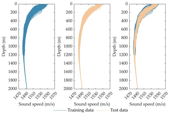
Figure 1. Training and test datasets.

2.2. Remote Sensing Parameter

Remote sensing sea surface parameters consist of SL and SST data. These data are sourced from the Copernicus Marine Environment Monitoring Service (CMEMS). The SL data are processed and disseminated by the DUACS altimeter processing system (https://doi.org/10.48670/moi-00148, accessed on 2 April 2025). By integrating satellite measurements from various altimeter missions, the global SL values are computed using the optimal interpolation method, with a spatial resolution of 0.25°. The SST data are obtained from the OSTIA global sea surface temperature data product (https://doi.org/10.48670/moi-00165, accessed on 2 April 2025). A data product with a spatial resolution of 0.05° is generated by integrating satellite observations and in situ measurement results. The remote sensing data all feature a daily time resolution, and a one-to-one correspondence is established with the SSP samples on the same day based on the principle of the closest distance.

2.3. Background Profile

In the SSP reconstruction, an SSP is generally expressed as the superposition of two components. One is the perturbation component, typically represented as the superposition of several order coefficients multiplied by the SSP basis functions. This reflects the temporal and spatial variations in the SSP. The other is the background profile, which is the constant part of the SSP and represents the stratification characteristics of the water column in the sea area. In the experiment, the data for the background profile are mainly extracted from the WOA23 dataset with a spatial resolution of 0.25° (https://www.ncei.noaa.gov/products/world-ocean-atlas, accessed on 2 April 2025). These data are the climatological mean values of the measured data from 1991 to 2020. In the inversion experiment, all data are interpolated to the standard sampling depths specified by the WOA23 dataset to ensure data depth consistency. For the depth sampling in the profile, the sampling interval was 5 m for the first 100 m, 25 m for the depth of 100–500 m, 50 m for the depth of 500–2000 m and 100 for the depth below 2000 m. In the inversion procedure, the WOA23 data serve as the background profile both for deriving the stratification characteristics of the sea area to compute the basis functions and for use in the SSP decomposition and reconstruction.

3. Method

3.1. SSP Basis Function

The primary challenge in achieving a full-depth SSP inversion lies in the scarcity of deep-depth samples. This scarcity makes it difficult to obtain the SSP basis functions using conventional statistical methods. Subsequently, an SSP basis function, which reflects the physical mechanism and does not require in situ samples, is derived from the perturbation modes of water protons in ocean.

Without taking into account the influence of the background flow, the perturbation of seawater protons can be described by the well-known Fjelsted equation:

$${\displaystyle \frac{d^{2}W}{d{z}^2}}+k^2{\displaystyle \frac{(N^2-{\sigma }^2)}{{\sigma }^2-f^2}}W=0,$$

(1)

where $W$ is the amplitude of the velocity of water protons moving in the vertical direction $z$. $k$ is the wave number in the horizontal direction, $\sigma$ is the frequency, $f$ is the Coriolis force, and $N$ is the buoyancy frequency. When the geostrophic effect is disregarded and the equivalent hydrostatic approximation is introduced, both $f$ and $\sigma$ can be regarded as approaching zero. The movement velocity of water protons is determined by the stratification characteristics $N$ of the seawater in the sea area, Equation (1) can be simplified as:

$${\displaystyle \frac{d^{2}W}{d{z}^2}}+{\displaystyle \frac{N^2}{{\nu }^2}}W=0,$$

(2)

where $\nu$ represents the phase velocity. For the actual continuously stratified ocean, the above equation can incorporate the condition that the sea surface and the sea floor are rigid boundaries. This transforms the problem into a classical Sturm–Liouville problem. Additionally, the variation in the eigenvalue with frequency can be disregarded, and the velocity amplitude $W$ can be expressed as:

$$W\left(z\right)={\sum }_j{\mu }_j{\phi }_j{e}^{i(k_{j}x+l_{j}y-\sigma t)},$$

(3)

where $\phi$ is the perturbation mode of water protons determined by the stratification characteristics of the water column. When $j$ equals zero, it corresponds to the barotropic mode, and when $j$ is greater than zero, it corresponds to the baroclinic mode. $l$ is the horizontal wavenumber, with the $x$-axis pointing east and the $y$-axis pointing north. $\mu$ is the coefficient corresponding to the mode.

The movement of seawater protons is the primary cause of the changes in the state of seawater. The variation in temperature $T$ can be expressed as:

$$∆T=W{\displaystyle \frac{dT}{dz}}.$$

(4)

Similarly to the SSP, the temperature profile can be represented as the superposition of a background profile $T_0$, which reflects the stable stratification characteristics of the representative sea area, and a $∆ T$, which represents the instantaneous perturbation. This can be derived by integrating Equation (4):

$$T\left(z,t\right)=T_0+{\displaystyle \frac{d{T}_0}{dz}}{\sum }_j{\displaystyle \frac{W_j}{i\sigma }}{\phi }_j{e}^{i(k_{j}x+l_{j}y-\sigma t)}.$$

(5)

The factors influencing the perturbation of the sound speed are the variations in the seawater temperature $T$ and salinity $S$. Among these, the change in sound speed induced by salinity is numerically much smaller than that caused by temperature. For a fixed depth, once the temperature rises by 1 °C, the sound speed increases by about 4.5 m/s, while for a 1 PSU increase in salinity, the corresponding increase in sound speed is only 1.5 m/s. Additionally, the salinity does not change significantly in the deep sea region. Thus, it is regarded that the temperature $T$ is the dominate cause of the SSP perturbation. For every 1 °C increase in temperature, the sound speed increases by approximately 4.5 m/s, showing an approximately linear relationship. The SSP $c\left(z\right)$ can be expressed as

$$c\left(z\right)=c_0+{\sum }_j{{\tau }_j\psi }_j,$$

(6)

where $c_0$ represents the background. The perturbation part is composed of the SSP basis function $\psi$ and its coefficient $\tau$. The expression of the physical basis function $\psi$ is presented as follows:

$${\psi }_j={\displaystyle \frac{d{T}_0}{dz}}{\phi }_j.$$

(7)

In the actual SSP inversion process, acquiring the SSP basis functions serves as the foundation of the inversion. Meanwhile, the corresponding coefficients are the inversion results used to reconstruct the SSP. The SSP basis functions proposed in this paper, which reflect the physical mechanism, overcome the reliance on in situ measurement samples. To calculate the SSP basis functions for the full depth of the sea area, only the background profile that describes the stratification characteristics of the sea area provided by data products such as WOA23 is required. Additionally, since these basis functions are based on the stratification characteristics of seawater, the reconstructed SSP must satisfy the physical constraints of the sea area’s stratification characteristics. This improves the rationality of deriving the full-depth profile from surface parameters.

3.2. Inversion Method

SOM is an artificial neural network characterized by a two-layer unsupervised competitive learning mechanism. It has been extensively applied in the domain of wide-area SSP inversion [12,13,14,15,16,17]. The reconstruction process of the full-depth SSP is illustrated in Figure 2. The following provides an introduction to the process in the sequence of implementation.

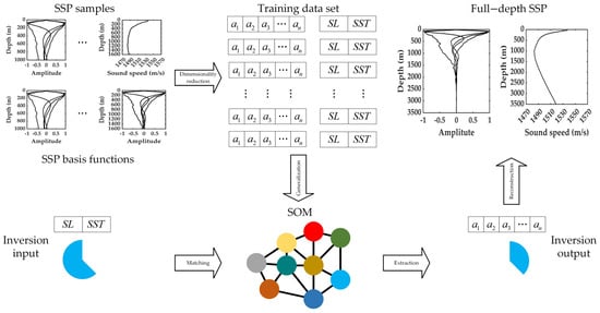
Figure 2. Flowchart of the inversion method.

Step 1: Dimensionality reduction. According to Equation (6), each SSP sample $c\left(z\right)$ is represented as a set of projection coefficients $a_n$. Given the actual perturbation scenario of the South China Sea’s SSPs, choosing five orders basis function for reconstruction can not only ensure an accurate depiction of the perturbation components but also avoid excessive noise introduced by high-order basis functions. To ensure consistency in the inversion process of ocean depth and perturbation modes, both the background profile and the corresponding basis functions are chosen as the values at the positions corresponding to the profile to be inverted. Theoretically, for all samples, regardless of the measurement depth, the projection coefficients of the basis functions can be obtained via regression analysis using the basis functions within the corresponding depth range. However, in actual tests, a large number of shallow-water samples (less than 400 m) from Argo tend to introduce outliers into the inversion process because of the significant perturbation of the upper-layer sound speed. This reduces the generalization ability of the inversion model. Considering that the depth of the sound channel axis in the South China Sea is approximately 1200 m, only profiles with a depth exceeding 1200 m are retained during training. This approach is adopted because the perturbations observed in the upper layer are more pronounced than those below 1200 m, and the depth sampling density is greater at shallower depths. Consequently, the method can not only avoid introducing excessive outliers but also ensure that the training samples contain important information related to the sound channel axis.

Step 2: Generalization. Combine the projection coefficients in the historical SSP samples with the corresponding remote sensing parameters SL and SST at the same time, longitude, and latitude into a 7-element array to construct a training vector. Input the training vector into the SOM algorithm to generate a generalized neural network topological structure, thereby forming a solution space. Through actual tests, it has been found that setting the number of neurons to three times that of the input training samples can ensure the accuracy of the inversion results [14,17]. Each neuron vector generated during training represents the possible SSP perturbation scenarios arising from the implicit relationship between the sea surface parameters and the projection coefficients in the training samples.

Step 3: Matching. The input for inversion consists of the sea surface remote sensing parameters SL and SST corresponding to the time and location of the SSP to be inverted. These two parameters constitute a neuron with incomplete elements. The best matching unit (BMU) is defined as the neuron vector on the neural network that has the minimum Euclidean distance from the incomplete input neuron. Chapman proposed the calculation method of the truncated Euclidean distance $d$ [12]:

$$d\left(x,u^p\right)={\sum }_{i\in avail}(1+{\sum }_{i\in missing}{({cor}_{ij}^c)}^2)\times (x_i-u_i^p),$$

(8)

where $p$ is the index number of neuron $u$ within the topology structure. The set $avail$ consists of available elements, which are the input parameters. The set $missing$ contains the missing elements, namely the coefficients of the SSP basis functions to be solved for. The matrix $cor$ is the covariance matrix among the parameters. Through the above formula, the Euclidean distances between the input parameters and all neurons in the solution space can be computed via the exhaustive method. Among these distances, the neuron with the smallest value is the BMU. This neuron represents the scenario that most closely corresponds to the relationships among the input parameters and the projection coefficients.

Step 4: Extraction. The inversion result is the elements of the corresponding miss set part in the BMU, that is, the projection coefficient elements. It represents a set of projection coefficients of the SSP basis functions that are most matched to the input remote sensing parameters in the space, solved based on the implicit relationships contained in the training sample vectors.

Step 5: Reconstruction. Once the projection coefficients of the SSP basis functions are obtained, the full-depth SSP results can be reconstructed using the full-depth background profile and the SSP basis functions of the sea area. Given that the data above 1200 m were mainly used in the training, the large-amplitude abnormal disturbances in the upper layer (especially above 400 m) and the shallow-layer data account for the vast majority of the variance contribution rate in the training samples, these factors will result in a slightly larger reconstructed value of the sound speed disturbance in the deep seawater. In fact, the sound speed values below 1200 m are essentially constant, and the sound speed gradient is the constant gradient of the deep-sea isothermal layer. Consequently, for depths greater than 1200 m, the reconstruction method primarily integrates the background profile value of the ocean bottom and employs the method of interpolating with a constant deep-sea isothermal layer gradient up to 1200 m. Briefly, the reconstruction results of the wide-area inversion method are utilized for the portion from the sea surface to the sound channel axis. For the part below the sound channel axis, reconstruction is carried out according to the characteristics of the deep-sea isothermal layer, taking into account the depth of the sound channel axis and the features of a constant gradient in the deep sea thermocline.

4. Result

Due to the severely limited number of full-depth SSP samples, the existing methods are unable to extract effective SSP basis functions for full-depth inversion and lack sufficient samples for full-depth inversion training. Consequently, no currently available method is capable of achieving wide-area full-depth inversion under practical application conditions. In applications such as acoustic field calculation where a full-depth profile is required, the most common approach is to utilize the climatological background profile provided by the WOA23 data. Consequently, in the subsequent result analysis, the accuracy of the inversion reconstruction results is mainly compared with that of the WOA23.

Figure 3 presents the reconstruction errors of all 247 profiles. A comparison is made between the inversion errors and those of the WOA23 profiles. It can be observed that the reconstruction errors of the vast majority of the inversion cases are smaller than those of the WOA23 profiles. Specifically, the average reconstruction error of the inversion is 2.85 m/s, while the average error of the WOA23 profiles is 3.26 m/s. In the absence of any in situ measurements, the error is decreased by approximately 13% via inversion processing when compared to directly using the WOA23 data. Typically, a root mean square error exceeding 4.5 m/s is regarded as a relatively large error result. When directly applying WOA23, the proportion of such cases reaches 16%. However, after inversion processing, this proportion decreases to 6%. From the perspective of reconstruction error, the inversion reconstruction method proposed in this paper is effective. By integrating data-driven approaches, the profiles obtained through inversion are closer to the actual sound speed distribution than the climatological mean profiles.

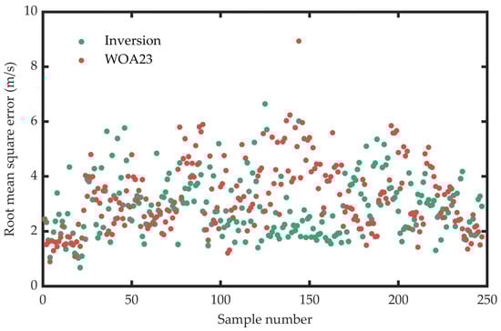
Figure 3. Reconstruction errors of all 247 profiles.

Figure 4 shows the variation in the SSP reconstruction error with depth. Consistent with the results in Figure 3, the inversion and reconstruction error are, at most depths, less than the background profile of WOA23. In the near-surface region, the improvement in the accuracy of the method is most evident. This is primarily because the input parameters are all surface parameters, which are most closely associated with the sound speed structure in the upper ocean. The maximum error of the two profiles occurs at a depth of approximately 100 m. This is attributed to the fact that the intersection of the mixed layer and the thermocline in the South China Sea generally lies within this depth range. The perturbation amplitude at this depth is extremely large within a single day. Even though the error is reduced by inverting the input surface parameters, the daily resolution characteristics of the parameters are insufficient to describe the large-scale temporal variations in the mixed layer. As the depth increases, the root mean square error of the SSP continuously diminishes. Especially at depths exceeding 1200 m, the errors of the two methods approach zero. This indicates that the error is proportional to the sound speed perturbation amplitude. As the depth increases, the sound speed approaches a constant value, resulting in a small inversion error. It should be noted that within the depth range of 1000 to 1500 m, compared with the WOA23 data, the inversion exhibits some small depth-dependent fluctuating errors. This is primarily attributed to the higher-order modes in the SSP basis function. Due to large-scale perturbations in the upper ocean, the higher-order modes introduce noise into the estimated values at greater depths. Nevertheless, this does not imply that directly using the WOA23 data is more accurate at greater depths. However, this does not imply that directly utilizing the WOA23 data is more precise at greater depths. Figure 5 presents the comparison of the estimated values of the sound channel axis depth obtained by the two methods. As WOA23 represents a historical average, the sound channel axis depth of the profile in the South China Sea remains constant. The average error from the actual sound channel axis is 358 m. After the inversion and reconstruction process, it is tantamount to correcting the background profile. Most of the errors of the estimated sound channel axis results are within 100 m. The sound channel axis depth is a critical parameter of the SSP, which directly determines the acoustic refraction structure. Thus, although introducing the SSP reconstruction may introduce some higher-order perturbation errors in the profile at greater depths, it can determine the sound channel axis depth more precisely compared to using the background profile. Consequently, when determining the maximum depth of the inversion sample processing in the inversion, a more advisable approach is to set it slightly greater than the sound channel axis of the sea area to ensure that the results can better represent the important sound channel axis structure.

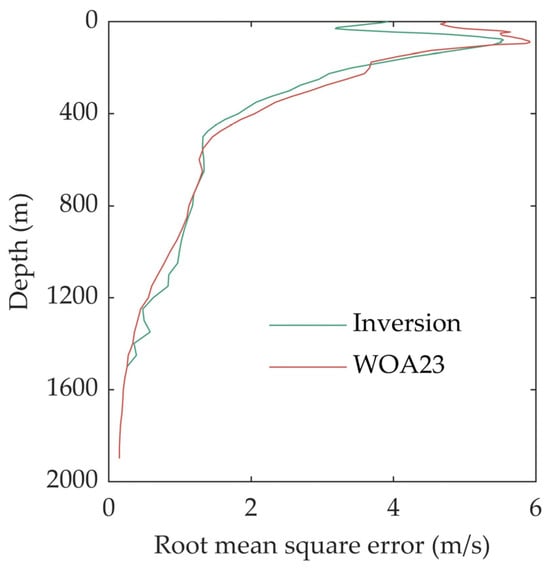
Figure 4. Reconstruction errors of different depths.

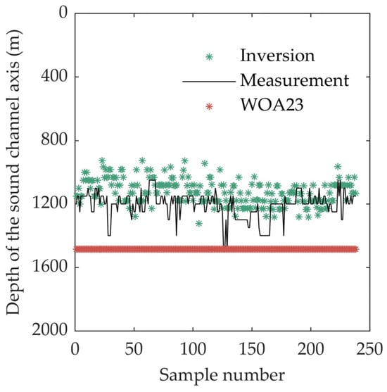
Figure 5. Comparison of the estimated values of the sound channel axis depth.

To obtain a deeper understanding of the effectiveness of SSP reconstruction, Figure 6 shows the reconstruction results of two typical profiles. The left figure shows the reconstruction result of a sample with the largest amplitude of the mixed layer perturbation relative to the background profile. The measurement time of this profile is 8 August 2021. Since the depth of the mixed layer is significantly greater than that of the background profile, the estimated values of both methods show relatively large errors. However, the inversion reconstruction method produces slightly better results compared to those of WOA23. As the depth increases, due to dynamic activities such as fronts, the SSP shows an obvious gradient change at a depth of approximately 500 m. This non-smooth gradient change is also difficult to describe using the current inversion method. As a result, both methods have relatively large errors. The right figure shows the reconstruction result of a sample featuring the most consistent mixed layer depth and background profile. The profile was measured on 7 April 2021. Within the mixed layer range, since the perturbation relative to the background profile is relatively minor, the differences between both methods and the measured profile are extremely small. The inversion reconstruction error within the thermocline is lower than that of the WOA23 profile. Meanwhile, the errors of both methods below the sound channel axis are very small because the perturbation below the sound channel axis is minimal. The measured profile also exhibits non-smooth sudden gradient changes at certain depths. This is a characteristic that is challenging to reconstruct with the current method and serves as a source of error in the reconstruction.

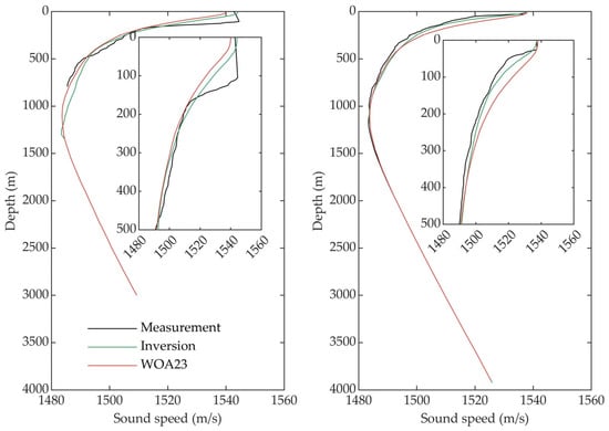
Figure 6. Reconstruction results of two typical profiles.

Since the calculation of the acoustic field is the most direct objective of obtaining the SSP, the accuracy of acoustic field prediction is also an important criterion for evaluating the reconstructed profiles. The profile in April shown in Figure 6 was chosen for acoustic field calculation verification. The sea depth at the measurement location of the SSP is 3900 m. The normal mode calculation model KRAKENC was employed to calculate the acoustic field. The source frequency is 100 Hz, and the depth is set at 60 m, where the estimation error of the SSP is relatively large. Typical South China Sea geoacoustic parameter values were used for the seabed. Specifically, the seabed sound speed is 1541 m/s, the density is 1.73 g/cm³, and the attenuation coefficient is 0.09 dB/λ.

Figure 7 shows the acoustic field prediction results of the two methods, along with their errors when compared to the predicted values of the measured profile. From these results, it is evident that the acoustic field calculation accuracy of the inversion method is significantly higher than that of the WOA23 profile. The average absolute error of the acoustic field predicted by the inversion method is 4.22 dB, while the corresponding error of the WOA23 profile is 5.79 dB. When comparing the interference structure of the measured SSP, both methods can yield a generally consistent interference structure. However, the WOA23 method fails to accurately describe the acoustic field interference structure at a depth of 2000 to 3000 m of a distance of approximately 40 km. Meanwhile, since the error in the SSP estimation mainly occurs at relatively shallow depths, the accuracy advantage of the inversion method is more prominent in the area above 100 m. Figure 8 shows the variation in the transmission loss with distance at a depth of 60 m. Within a distance of 50 km, the average transmission loss prediction error of the inversion SSP is 2.50 dB, whereas the prediction error of the WOA23 profile is 5.96 dB. Although, from the perspective of the SSP reconstruction, the accuracy of the inversion method has been improved by approximately 13%, the effectiveness of its acoustic field calculation has been significantly enhanced due to the correction of key parameters such as the depth of sound channel axis. Within a distance of 20 km, both methods can accurately depict the acoustic field interference structure. As the distance increases and errors accumulate continuously, the acoustic field prediction error of the WOA23 method keeps rising. When the distance reaches 50 km, the result of the WOA23 profile can no longer accurately represent the acoustic field interference structure, and the error from the actual value approaches nearly 30 dB, while the error of the inversion is approximately 4 dB. From the perspective of practical applications, the inversion SSP can meet the requirements of many practical applications within a range of 50 km.

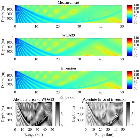
Figure 7. Acoustic field prediction results.

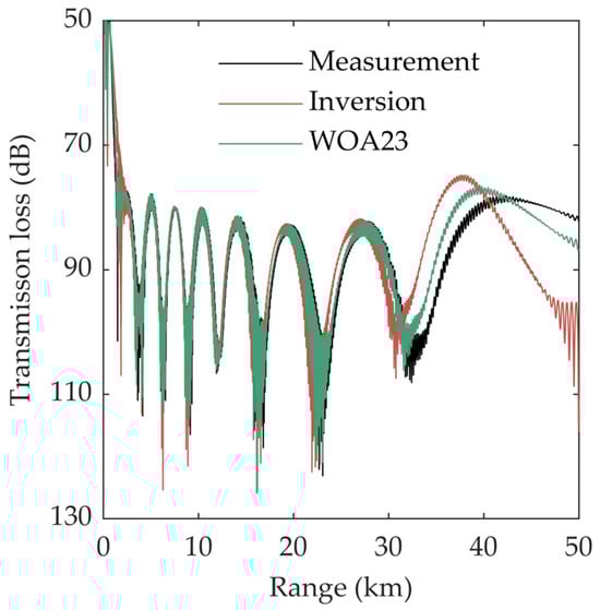
Figure 8. Predicted value of transmission loss at 60 m.

5. Conclusions

Owing to the scarcity of full-depth SSP samples and the high uncertainty of statistical methods in predicting when sample quantities are insufficient, traditional methods face challenges in achieving full-depth SSP estimation. To address this issue, two physical mechanism constraints are integrated based on the classical SOM inversion. Firstly, a physically based SSP basis function is derived from the proton perturbation modes of seawater. By utilizing data products such as WOA23 to obtain the background profile, the full-depth SSP basis function for the inversion area can be obtained, laying a foundation for modeling the full-depth SSP perturbation. Secondly, the inversion of the SSP above the sound channel axis is achieved by combining limited-depth samples with the full-depth SSP basis function. Subsequently, the reconstruction of the SSP in the deep-sea isothermal layer is completed by integrating it with the deep-sea ideal SSP structure model. By incorporating physical mechanism constraints, effective profile extrapolation is achieved based on limited-depth samples. Moreover, wide-area full-depth SSP inversion is accomplished by using remote sensing data as the input.

Through the SSP inversion and reconstruction experiments using Argo profiles and corresponding remote sensing data in the South China Sea from 2007 to 2024, the effectiveness of the proposed method was verified. Based on the inversion method, the full-depth SSP was effectively reconstructed. The average error compared with the measured data is 2.85 m/s, and the estimation accuracy of key parameters such as the depth of the sound channel axis has been improved compared with the climatological mean profile. Since the wide-area inversion method uses sea surface parameters as input parameters, it can estimate the structure of the upper ocean SSP more accurately. However, limited by factors such as the temporal resolution of the data, the main sources of error are the large-scale perturbation of the SSP structure caused by the mixed layer depth and the sudden non-smooth gradient changes at certain depth. The results of the acoustic field prediction based on the reconstructed SSP indicate that the accuracy of the results can meet the requirements of acoustic field calculation applications, and the transmission loss error within 50 km is less than 5 dB. Compared with using the climatological mean profile in the WOA23 data, the inversion method can provide more effective acoustic field calculation results.

Although there is a certain discrepancy in accuracy when compared with methods for estimating the SSP based on in situ measured data such as acoustic tomography, the wide-area SSP inversion method based on sea surface parameters can offer effective SSP information without any in situ measurements, rendering it highly practical. In previous attempts to invert the SSP using remote sensing sea surface parameters, full-depth inversion was not achievable. By relying on data products such as the WOA23, the proposed wide-area technology allows for acquisition of the full-depth SSP. Given that satellite remote sensing platforms offer quasi-real-time global observational data as input, and processing a series of profiles using MATLAB R2024a on a laptop requires only minutes to a few hours, the methodology presented here can, in principle, deliver near-real-time global SSP information, thus supporting applications in acoustic field computation. In subsequent research, the relevant method can be further refined to enhance the accuracy of obtaining the full-depth SSP from aspects such as incorporating measured data and acquiring more precise stratification information of the inversion sea area. When derived from in situ measurements of ocean stratification, the ability of physical basis functions to accurately capture oceanic dynamic processes at short time scales requires further validation.

References

- Li, H.; Huang, J.; Xu, Z.; Yang, K.; Qin, J. Broadband source localization using asynchronous distributed hydrophones based on frequency invariability of acoustic field in shallow water. Remote Sens. 2024, 16, 982. [Google Scholar] [CrossRef]
- Wang, Y.; Zhu, J.; Zhang, M.; Tu, X.; Wei, Y.; Qin, H.; Qu, F. PBiGAMP-based joint channel estimation and data detection under nonuniform doppler shifts. IEEE J. Ocean. Eng. 2025, 50, 3087–3105. [Google Scholar] [CrossRef]
- Peng, Y.; Li, H.; Zhang, W.; Zhu, J.; Liu, L.; Zhai, G. Underwater sonar image classification with image disentanglement reconstruction and zero-shot learning. Remote Sens. 2025, 17, 134. [Google Scholar] [CrossRef]
- Ma, T.; Zhang, T.; Xu, W. Path Identification in passive acoustic tomography via time delay difference comparison and accumulation analysis. J. Mar. Sci. Eng. 2025, 13, 1996. [Google Scholar] [CrossRef]
- Xiao, C.; Zhu, X.; Zhang, C.; Zhu, Z.; Ma, Y.; Zhong, J.; Wei, L. Coastal acoustic tomography system for monitoring transect suspended sediment discharge of Yangtze river. J. Hydrol. 2025, 623, 129832. [Google Scholar] [CrossRef]
- Carnes, M.R.; Mitchell, J.L.; de Witt, P.W. Synthetic temperature profiles derived from geosat altimetry: Comparison with air-dropped expendable bathythermograph profiles. J. Geophys. Res. 1990, 95, 17979–17992. [Google Scholar] [CrossRef]
- Carnes, M.R.; Teague, W.J.; Mitchell, J.L. Inference of Subsurface Thermohaline Structure from Fields Measurable by Satellite. J. Atmos. Ocean. Technol. 1994, 11, 551–566. [Google Scholar] [CrossRef]
- Fox, D.N.; Teague, W.J.; Barron, C.N.; Carnes, M.R.; Lee, C.M. The Modular Ocean Data Assimilation System (MODAS). J. Atmos. Ocean. Technol. 2002, 19, 240–252. [Google Scholar] [CrossRef]
- Peter, C.C.; Wang, G.; Fan, C. Evaluation of the U.S. Navy’s Modular Ocean Data Assimilation System (MODAS) using South China Sea monsoon experiment (SCSMEX) data. J. Oceanogr. 2004, 60, 1007–1021. [Google Scholar] [CrossRef]
- Chen, C.; Ma, Y.; Liu, Y. Reconstructing sound speed profiles worldwide with sea surface data. Appl. Ocean Res. 2018, 77, 26–33. [Google Scholar] [CrossRef]
- Su, H.; Yang, X.; Lu, W.; Yan, X. Estimating subsurface thermohaline structure of the global ocean using surface remote sensing observations. Remote Sens. 2019, 11, 1598. [Google Scholar] [CrossRef]
- Charantonis, A.A.; Testor, P.; Mortier, L.; D’Ortenzio, F.; Thiria, S. Completion of a sparse glider database using multi-iterative self-organizing maps (ITCOMP SOM). Proc. Comput. Sci. 2015, 51, 2198–2206. [Google Scholar] [CrossRef]
- Chapman, C.; Charantonis, A.A. Reconstruction of Subsurface velocities from satellite observations using iterative self-organizing maps. Geosci. Remote Sens. Lett. 2017, 14, 617–620. [Google Scholar] [CrossRef]
- Ou, Z.; Qu, K.; Wang, Y.; Zhou, J. Estimating sound speed profile by combining satellite data with in situ sea surface observations. Electronics 2022, 11, 3271. [Google Scholar] [CrossRef]
- Liu, Y.; Chen, W.; Chen, Y.; Meng, Z. Research progress on methods for constructing underwater sound speed profile. Inf. Countermeas. Technol. 2022, 3, 1–18. [Google Scholar] [CrossRef]
- Cheng, C.; Yan, F.; Gao, Y.; Jin, T.; Zhou, Z. Improving reconstruction of sound speed profiles using a self-organizing map method with multi-source observations. Remote Sens. Lett. 2020, 11, 572–580. [Google Scholar] [CrossRef]
- Xu, G.; Qu, K.; Li, Z.; Zhang, Z.; Xu, P.; Gao, D.; Dai, X. Enhanced inversion of sound speed profile based on a physics-inspired self-organizing map. Remote Sens. 2025, 17, 132. [Google Scholar] [CrossRef]
- Zhang, Z.; Qu, K.; Li, Z. A statistical optimization method for sound speed profiles inversion in the South China Sea based on acoustic stability pre-clustering. Appl. Sci. 2025, 15, 8451. [Google Scholar] [CrossRef]
- Shaikh, S.; Huang, Y.; Alharbi, A.; Bilal, M.; Shaikh, A.S.; Zuberi, H.H.; Dars, M.A. Acoustic propagation and transmission loss analysis in shallow water of northern Arabian Sea. J. Mar. Sci. Eng. 2024, 12, 2256. [Google Scholar] [CrossRef]
- Zhang, W.; Jin, S.; Gang, B.; Yang, C.; Peng, C.; Xia, H. A method for sound speed profile prediction based on CNN-BiLSTM-attention network. J. Mar. Sci. Eng. 2024, 12, 414. [Google Scholar] [CrossRef]
- Huang, W.; Lu, J.; Lu, J.; Wu, Y.; Zhang, H.; Xu, T. STNet: Prediction of underwater sound speed srofiles with an advanced semi-transformer neural network. J. Mar. Sci. Eng. 2025, 13, 1370. [Google Scholar] [CrossRef]
- Bianco, M.; Gerstoft, P. Dictionary learning of sound speed profiles. J. Acoust. Soc. Am. 2017, 141, 1749–1758. [Google Scholar] [CrossRef]
- Cheng, L.; Ji, X.; Zhao, H.; Li, J.; Xu, W. Tensor-based basis function learning for three-dimensional sound speed fields. J. Acoust. Soc. Am. 2022, 151, 269–285. [Google Scholar] [CrossRef]
- Li, Z.; Liu, Z.; Lu, S. Global Argo data fast receiving and post-quality-control system. IOP Conf. Ser. Earth Environ. Sci. 2020, 502, 012012. [Google Scholar] [CrossRef]
- Del Grosso, V.A. New equation for the speed of sound in natural waters (with comparisons to other equations). J. Acoust. Soc. Am. 1974, 56, 1084–1091. [Google Scholar] [CrossRef]
Disclaimer/Publisher’s Note: The statements, opinions and data contained in all publications are solely those of the individual author(s) and contributor(s) and not of MDPI and/or the editor(s). MDPI and/or the editor(s) disclaim responsibility for any injury to people or property resulting from any ideas, methods, instructions or products referred to in the content. |
© 2026 by the authors. Licensee MDPI, Basel, Switzerland. This article is an open access article distributed under the terms and conditions of the Creative Commons Attribution (CC BY) license.