Article

Automated Recognition of Rock Mass Discontinuities on Vegetated High Slopes Using UAV Photogrammetry and an Improved Superpoint Transformer

1
Changjiang River Scientific Research Institute, Wuhan 430010, China
2
Research Center on Water Engineering Safety and Disaster Prevention of MWR, Wuhan 430010, China
3
Research Center on National Dam Safety Engineering Technology, Wuhan 430010, China
*
Author to whom correspondence should be addressed.
Remote Sens. 2026, 18(2), 357; https://doi.org/10.3390/rs18020357
Submission received: 28 November 2025 / Revised: 8 January 2026 / Accepted: 13 January 2026 / Published: 21 January 2026

Highlights

What are the main findings?
  • Integrated close range UAV photogrammetry with an improved Superpoint Transformer to segment rock and vegetation on steep vegetated slopes.
  • VDVI and volumetric density features with hierarchical filtering achieved 89.5 percent overall accuracy, 25 times faster processing, and automatically extracted discontinuity planes with key geometric parameters.
What are the implications of the main findings?
  • Enables rapid, safe discontinuity mapping for hazardous high slopes, reducing field exposure while preserving centimetre scale geometric detail for engineering decisions.
  • Delivers orientation, spacing, persistence, and trace statistics to support slope stability evaluation, rockfall hazard screening, and digital geotechnical inventories in vegetation covered terrains.

Abstract

Automated recognition of rock mass discontinuities in vegetated high-slope terrains remains a challenging task critical to geohazard assessment and slope stability analysis. This study presents an integrated framework combining close-range UAV photogrammetry with an Improved Superpoint Transformer (ISPT) for semantic segmentation and structural characterization. High-resolution UAV imagery was processed using an SfM–MVS photogrammetric workflow to generate dense point clouds, followed by a three-stage filtering workflow comprising cloth simulation filtering, volumetric density analysis, and VDVI-based vegetation discrimination. Feature augmentation using volumetric density and the Visible-Band Difference Vegetation Index (VDVI), together with connected-component segmentation, enhanced robustness under vegetation occlusion. Validation on four vegetated slopes in Buyun Mountain, China, achieved an overall classification accuracy of 89.5%, exceeding CANUPO (78.2%) and the baseline SPT (85.8%), with a 25-fold improvement in computational efficiency. In total, 4918 structural planes were extracted, and their orientations, dip angles, and trace lengths were automatically derived. The proposed ISPT-based framework provides an efficient and reliable approach for high-precision geotechnical characterization in complex, vegetation-covered rock mass environments.

1. Introduction

High-slope rock masses often contain discontinuities such as joints, fractures, and bedding planes, which govern mechanical stability and play a crucial role in geotechnical hazard assessment [1]. Accurate identification and parameterization of these discontinuities are essential for slope stability evaluation and rockfall hazard mitigation [2]. Conventional field-based measurements are labor-intensive, pose safety risks, and fail to capture the full spatial complexity of inaccessible cliffs [3]. Alternative ground-based remote sensing methods, such as TLS (Terrestrial Laser Scanning), provide high precision but remain limited in coverage, cost efficiency, and occlusion handling [4]. Recent advances in UAV-based photogrammetry—via Structure-from-Motion (SfM) combined with Multi-View Stereo (MVS)—enable centimeter-level 3D mapping of challenging terrains, reconstructing large-area dense point clouds with minimal ground control [5]. Terrestrial LiDAR can precisely map rock geometry by active ranging, and these two methods are complementary: UAV photogrammetry is cost-effective and high-resolution but does not directly measure ranges and may be sensitive to lighting, whereas TLS provides direct ranging but is limited by occlusion, logistics, and cost [6,7].
Data processing serves as the core of non-contact rock mass geometric structure feature extraction for both ground-based and UAV platforms. The 3D point cloud—derived from LiDAR scanning or photogrammetry—is the preferred data modality for extracting geometric structure features of rock masses. Extracting planes from 3D point clouds represents a key algorithm [8], while geometric structure parameter extraction forms the foundation for rock mass stability analysis. For rock mass discontinuity plane extraction from 3D point clouds, geometry-driven segmentation pipelines remain the mainstream; however, their performance is sensitive to noise, roughness, and uneven sampling on steep outcrops. Additionally, vegetation occlusion increases the difficulty of rock mass plane extraction, and the classification of vegetation and rock point clouds remains a major challenge [9,10,11]. The following subsections review the main algorithms involved in rock mass geometric structure feature extraction.

1.1. Point-Cloud-Based Structural Plane Extraction

Using 3D models or dense point clouds extracted via unmanned aerial vehicle (UAV) photogrammetry for slope monitoring has seen numerous studies and applications to date [12], enabled by widespread open-source and commercial software solutions [13]. Outputs from these studies enabled basic extraction of discontinuity orientations via manual interpretation or semi-automated plane fitting [14]. Techniques evolved from manual fitting to normal-based clustering and segmentation, often relying on local PCA and RANSAC, later enhanced by density-based segmentation algorithms like DBSCAN [15]. Concurrently, integration of multi-sensor data, including LiDAR and SfM point clouds from UAV-borne or ground-based devices, enhanced completeness and accuracy in complex geometries [16]. However, the semantic interpretation of point clouds in vegetated environments remains hindered by occlusion and pronounced inter-class similarity [17].
Commercial tools like Agisoft Metashape and CloudCompare are widely used to process UAV survey data (direct LiDAR point clouds or SfM-reconstructed clouds) and generate accurate Digital Terrain Models (DTMs) and outcrop meshes [18]. After isolating pure rock point clouds, structural planes and geometric parameters are derived via a standard pipeline: first, point normals are estimated (e.g., local PCA, Hough voting); second, points are clustered by normal direction to group coplanar patches [19]; finally, plane equations are fitted via RANSAC. For example, Pola et al. (2024) [20] optimized this pipeline by applying k-means clustering on point normals, refining clusters using a k-nearest-neighbor filter, and separating distant clusters via DBSCAN before RANSAC fitting. A multi-scale regional Mask R-CNN also achieved superior accuracy for automatic cavity instance segmentation on digital outcrop images of the Dengying Formation [21]. Other strategies use cumulative distributions of normal or elevation histograms to find dominant dip/dip-direction sets [22]. Overall, recent reviews note that these geometric methods, when applied to high-quality UAV or LiDAR clouds, can reliably recover the main joint sets and structural parameters [23].

1.2. Vegetation Separation and Classification in Point Clouds

Vegetation occlusion remains a critical bottleneck for high-slope rock mass analysis: it obscures rock surfaces, complicates structural extraction, and requires dedicated filtering or point-cloud classification to isolate rock points [24]. Traditional approaches to vegetation removal use intensity/color thresholds, radiometric indices, or morphological filters [25], while more sophisticated methods frame vegetation classification as a machine learning problem [26]. Representative workflows include 2D UAV image segmentation via U-Net (classifying “vegetation” or “ground” pixels) followed by 3D point cloud projection—effectively stripping seasonal foliage [27]—and 3D deep learning methods that learn features directly from point clouds. 3D learning techniques (e.g., PointNet, PointNet++, 3D CNNs) have become standard for end-to-end semantic segmentation (trees, soil, rock) with accuracies exceeding 90% in forested terrain [28]. For example, Pinto et al. (2020) [29] applied a multichannel Convolutional Neural Network (using FPFH and color histograms on small 3D patches) to classify points into categories like bush, grass, and bare earth, while Fan et al. (2023) [30] used PointNet++ for high-accuracy (≈92%) vegetation classification from LiDAR. Han et al. (2024) [31] further introduced WHU-Urban3D—a large-scale urban LiDAR point-cloud dataset integrating airborne (ALS) and mobile (MLS) scanning with per-point annotations—establishing a standardized benchmark for 3D urban-scene understanding.
Recent advances have introduced transformer-based architectures and hybrid UAV survey systems that integrate multi-modal data, such as thermal and RGB imagery, for long-term landslide monitoring [32]. In parallel, weakly supervised LiDAR models have been developed to predict vegetation stratum occupancy, showing strong potential for application in rock–vegetation segmentation tasks [33]. Collectively, these 3D learning techniques are enabling more automated and robust vegetation filtering, gradually replacing traditional machine learning methods such as support vector machines and random forests that rely on hand-crafted features. Nevertheless, deep learning approaches require large volumes of high-quality labeled “rock versus vegetation” data, which are costly and time-consuming to obtain, and they continue to face challenges related to overfitting, limited generalizability, and domain shifts arising from heterogeneous terrain and sensor conditions [34].
As summarized in Table 1, representative studies indicate that UAV photogrammetry and point cloud learning methods can enable remote discontinuity mapping and vegetation handling, but their performance remains constrained by point cloud quality, vegetation occlusion, and data or parameter requirements.

1.3. Objective of This Study

Building upon these developments, this study introduces an Improved Superpoint Transformer (ISPT) framework tailored for discontinuity recognition in vegetated high-slope terrains. The proposed approach incorporates three major innovations: (i) feature augmentation with volumetric density and Visible-band Difference Vegetation Index (VDVI) for vegetation discrimination, (ii) hierarchical filtering using Cloth Simulation Filter and vegetation thresholding to mitigate occlusion, and (iii) connected component segmentation to accelerate superpoint generation. Experimental validation on four vegetated slopes demonstrates significant improvements in classification accuracy and computational efficiency compared to traditional geometric methods and existing deep learning baselines.

2. Methodology

2.1. Data Acquisition

Four hazardous rock slopes located in Buyun Mountain, China, were surveyed using a DJI Mini 4 Pro (SZ DJI Technology Co., Ltd., Shenzhen, China) UAVequipped with a 48 MP RGB camera. The UAV flew close to the high-slope surface. Flight planning targeted >90% overlap in both elevation direction and cross-slope direction. Given the close-range imaging distance of ~3–6 m and the camera specifications (48 MP, 8064 × 6048), the effective GSD is on the order of sub-millimeter to ~1 mm per pixel (approximately 0.5–1.1 mm/px), depending on the site and camera-to-slope distance.
Ground control points (GCPs) were deployed not only for georeferencing the photogrammetric products, but also to verify the relative geometric accuracy of the reconstructed 3D model and derived point cloud. The GCP targets were created directly on the rock surface by applying a stencil template and spray paint to produce clear, high-contrast markers suitable for image identification and measurement. At each site, a total of three ground control points (GCPs) were deployed for bundle adjustment and absolute georeferencing, and two independent checkpoints (CPs) were reserved for accuracy assessment. All control and checkpoints were surveyed using a real-time kinematic (RTK) GNSS approach, with a nominal measurement accuracy of approximately 1.5 cm. The photogrammetric models were referenced to the China Geodetic Coordinate System 2000 (CGCS2000), and all reported positions and residual statistics for georeferencing/validation were evaluated in this coordinate framework.
In total, 1412 images were captured, producing 13.4 GB of raw imagery. The photos were processed using an SfM–MVS photogrammetric workflow technique to generate 3D models and dense point clouds. The four study areas are designated as Study Area 1 to Study Area 4. Figure 1 shows the close-up images of the high-slope rock mass in Study Area 4. It can be observed from the figure that the study area is covered with relatively abundant vegetation. The vegetation coverage in the other three study areas is similar to that in Study Area 4.

2.2. Data Preprocessing

2.2.1. The Overall Workflow

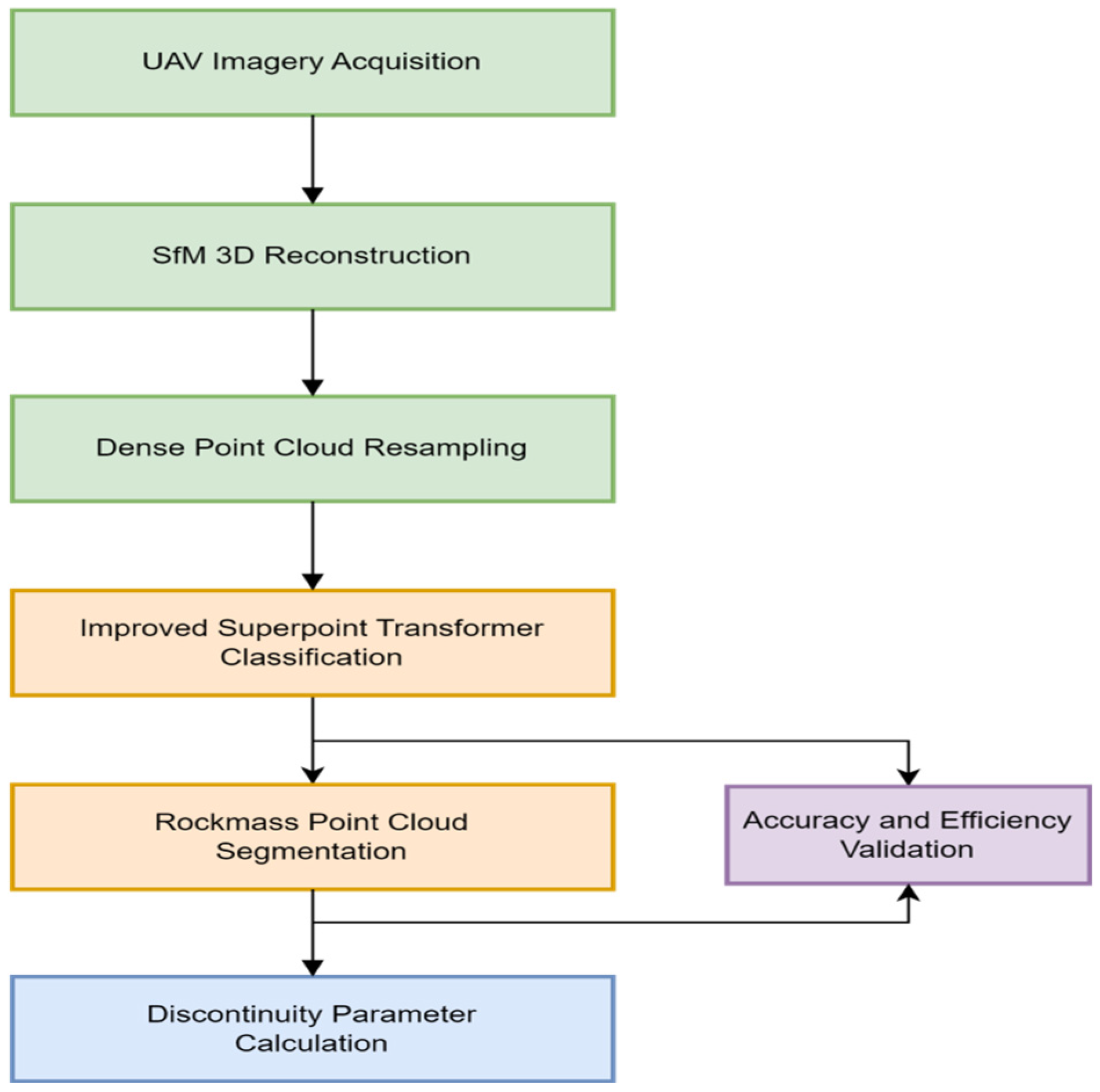
This study proposes a novel framework for automated rock mass discontinuity recognition on vegetated high slopes using UAV photogrammetry. The proposed workflow integrates UAV-based photogrammetry, advanced semantic segmentation, and geometric analysis for automated rock mass discontinuity recognition. It consists of five major components: (1) high-resolution data acquisition using UAVs, (2) 3D model reconstruction via SfM, (3) connected-component-based superpoint generation, (4) feature-augmented semantic segmentation using the ISPT model, and (5) structural parameter extraction. Finally, validation is performed through comparison with manual field measurements and statistical evaluation of classification accuracy metrics. This pipeline addresses the challenges of dense vegetation and complex slope geometry by combining advanced photogrammetric techniques with state-of-the-art deep learning models. Figure 2 illustrates the overall workflow of this study.

2.2.2. SfM–MVS 3D Reconstruction

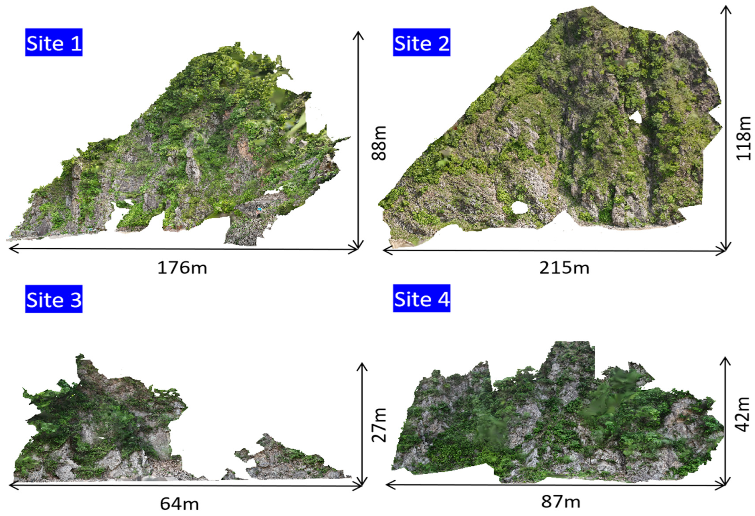
A Structure-from-Motion pipeline was employed to compute camera poses and reconstruct sparse point clouds, followed by Multi-View Stereo densification to generate high-fidelity 3D point clouds. Drone-based SfM workflows are particularly advantageous for surveying large or inaccessible areas, offering high-resolution, georeferenced 3D reconstructions with minimal ground-based intervention. Figure 3 shows the schematic diagram of the three-dimensional reconstruction results of the four rock masses in this study.
In this study, we follow a conventional SfM–MVS photogrammetric pipeline. The SfM stage is used to estimate camera orientations and reconstruct a sparse point cloud (tie points), while the subsequent MVS stage performs dense image matching to generate the dense point cloud used for geometric analysis. A surface mesh can then be reconstructed from the dense cloud for visualization and surface regularization. For downstream ISPT processing, we optionally resample the reconstructed mesh into a uniformly sampled surface point cloud (with inherited color/normal attributes) to control redundancy and improve computational efficiency; importantly, this mesh-to-point conversion is performed after dense reconstruction and does not imply that a 3D model is generated directly from the sparse SfM output.
The photogrammetric 3D reconstruction stage is computationally intensive. We commissioned this step to a professional photogrammetry service provider equipped with dedicated high-performance computing resources.

2.2.3. Dense Point-Cloud Export and Mesh-to-Point Resampling

Converting a 3D model into a point cloud provides a flexible and efficient data format suitable for a wide range of applications. By eliminating redundant topology, point clouds offer a lightweight representation that simplifies data storage and processing. Their unstructured nature allows greater adaptability for segmentation, filtering, and transformation operations, while enabling efficient execution of feature extraction, clustering, and geometric analysis. In addition, point clouds are highly compatible with modern machine learning workflows, facilitating advanced tasks such as object detection and semantic segmentation.
The conversion of an oblique photogrammetric 3D model into a point cloud follows a systematic procedure designed to preserve both geometric fidelity and visual detail. The process begins with mesh decimation to reduce model complexity, followed by uniform surface sampling to generate discrete spatial points. Color and normal attributes are then mapped to maintain texture and surface orientation information, while noise reduction filters are applied to remove photogrammetric artifacts. Optional densification steps can further enhance spatial resolution. Finally, the point cloud is aligned and scaled to ensure consistency with geospatial references. This workflow yields a geometrically accurate and radiometrically consistent point cloud, suitable for downstream applications such as structural characterization and quantitative feature extraction.

2.2.4. Outlier and Noise Removal

After converting the oblique photogrammetric 3D model into a surface point cloud, the converted point cloud can still contain abnormal points and noisy fragments. These artifacts are mainly introduced by image-matching ambiguities during SfM–MVS reconstruction and are often concentrated near sharp edges, occlusion boundaries, low-texture regions, and vegetation-covered areas; they may be further emphasized by mesh-to-point sampling. Therefore, we applied a dedicated denoising procedure to the converted point cloud prior to ISPT-based rock–vegetation classification.
First, we removed invalid points and performed a neighborhood-statistics-based Statistical Outlier Removal (SOR) to suppress sparse “floating” points. For each point, the mean distance to its k nearest neighbors was computed, and points whose mean neighbor distance exceeded a global threshold were rejected. Following the commonly used default settings in CloudCompare (v2.13.2), the SOR parameters were set to k = 20 and a standard-deviation multiplier of 2.0, which effectively removed isolated outliers while preserving the geometric continuity of rock surfaces.
Second, a complementary Radius Outlier Removal (ROR) was applied to eliminate residual isolated points by requiring at least N neighbors within a sphere of radius r. Based on the typical sampling density of the converted cloud and common practice for close-range photogrammetric point clouds, r was set to 0.05 m, and N was set to 6 to balance noise suppression and detail preservation.
Third, to reduce local high-frequency surface noise while retaining planar rock faces, we performed a local plane-consistency check: for each point, a best-fitting plane was estimated from its neighborhood, and points whose orthogonal distance to the fitted plane exceeded 0.02 m were removed.
Finally, small disconnected fragments were suppressed using a connected-component cleanup. Euclidean connected components were identified with a connectivity tolerance of 0.05 m, and components smaller than 200 points were discarded, as these fragments are typically associated with residual mismatches or vegetation-induced artifacts rather than continuous rock surfaces. After these steps, the denoised point cloud was used as the input for subsequent hierarchical filtering and ISPT semantic segmentation.

2.3. Rock and Vegetation Point Cloud Classification

2.3.1. The SPT Algorithm

In this study, we employed an improved Superpoint Transformer (SPT) algorithm for the classification of vegetation and rock point clouds.
The Superpoint Transformer (SPT) algorithm was introduced in 2023 by Damien Robert, Hugo Raguet, and Loic Landrieu [39]. It is a cutting-edge method designed for efficient semantic segmentation of large-scale 3D point clouds. The algorithm combines a hierarchical superpoint structure with transformer-based self-attention mechanisms to process 3D data effectively.
The SPT algorithm begins by partitioning a 3D point cloud into geometrically homogeneous regions, termed superpoints, using an innovative and fast hierarchical partitioning algorithm. This preprocessing step can be up to seven times faster than previous superpoint-based methods. The hierarchical partition organizes superpoints across multiple scales, adapting to local geometric and radiometric complexity. In the SPT algorithm, the features used for segmenting point clouds into superpoints include RGB, curvature, planarity, scattering, verticality, and elevation derived from PCA of local neighborhoods and radiometric properties. A k-nearest neighbor graph is constructed to model spatial adjacency, and a parallelized graph-cut algorithm is applied to generate multi-scale partitions by aggregating points into coarser superpoints through mean pooling. For ground point filtering, the method uses RANSAC to robustly estimate a ground plane from coarsely subsampled points.
After partitioning the point cloud into hierarchical superpoints, the paper processes these superpoints through a transformer-based architecture. The transformer architecture in the SPT algorithm employs a sparse self-attention mechanism to learn relationships between superpoints at these scales, enabling efficient modeling of long-range interactions. This approach processes millions of points simultaneously by classifying a reduced set of superpoints, eliminating the need for computationally intensive sliding windows or voxel grids.

2.3.2. Improvements of the SPT Algorithm (ISPT)

The ISPT model improves upon the baseline SPT by incorporating VDVI and volumetric density features into the input representation. Preprocessing includes hierarchical filtering with the Cloth Simulation Filter (CSF) for ground removal and VDVI-based vegetation filtering. Connected component analysis is applied to partition the point cloud into spatially coherent clusters prior to hierarchical superpoint segmentation. These superpoints are processed by a transformer encoder–decoder architecture employing sparse attention for efficient global context modeling. The semantic segmentation output distinguishes rock and vegetation points, achieving robust performance under dense foliage.
(i)
Feature Augmentation
The original SPT algorithm relies on geometric features such as planar curvature and normal vectors. To enhance discriminative power in vegetated slopes, we introduce two new features: volumetric density and the Visible-Band Difference Vegetation Index (VDVI) [40]. Volumetric density is defined as the number of points per unit volume within a moving window, capturing the spatial clustering of rock mass and vegetation. Mathematically, it is expressed as follows:
ρ v = N Δ V
where N is the number of points in a voxel of volume Δ V . High volumetric density indicates compact rock mass, while low density corresponds to sparse vegetation or voids.
The Visible-Band Difference Vegetation Index (VDVI), computed from UAV-derived RGB imagery, enhances vegetation discrimination by accentuating the green channel relative to red and blue components:
V D V I = 2 G R B 2 G + R + B
where R, G, and B are the red, green, and blue channel values. Points with high VDVI values are classified as vegetation, enabling vegetation-rock discrimination.
Vegetation detection via the VDVI capitalizes on distinct spectral signatures to differentiate vegetation from other objects. Vegetation demonstrates unique reflectance patterns across different wavelengths: it typically exhibits higher reflectance in the green region and lower reflectance in the red and blue spectral bands. By leveraging these spectral disparities, VDVI enhances the separability between vegetative and non-vegetative targets. Comparative studies have shown that VDVI outperforms traditional vegetation indices by reducing spectral overlap between vegetation and non-vegetation classes.
(ii)
Hierarchical Filtering
Prior to superpoint segmentation, we implement a two-stage filtering pipeline to reduce noise and vegetation interference. This combination effectively separates vegetated overhangs and rocky outcrops from the underlying terrain. First, a Cloth Simulation Filter (CSF) for ground removal. CSF refers to the Cloth Simulation Filter algorithm for ground filtering based on cloth simulation [41]. Its fundamental principle involves the process of gradually conforming a computer-simulated cloth to ground points.
CSF filtering is followed by a VDVI-based vegetation filter that thresholds and removes dense vegetation points, reducing vegetation density by up to 60%. Points with a VDVI greater than 0.05 are regarded as vegetation points and filtered out at this step.
(iii)
Connected Component Segmentation
To improve superpoint segmentation efficiency, we incorporate connected component analysis (CCA) as a preprocessing step. CCA groups points into clusters based on Euclidean distance connectivity, creating preliminary segments that align with physical objects (e.g., rock blocks, vegetation clumps). This reduces the computational complexity of subsequent superpoint generation by breaking the point cloud into manageable subregions. For point clouds, connected components represent collections of spatially adjacent points, and the proximity of points is inherently related to point cloud density. Therefore, connected component segmentation of point clouds can, to some extent, be classified as a density-based segmentation method.

2.3.3. The Overall Workflow of the ISPT Algorithm

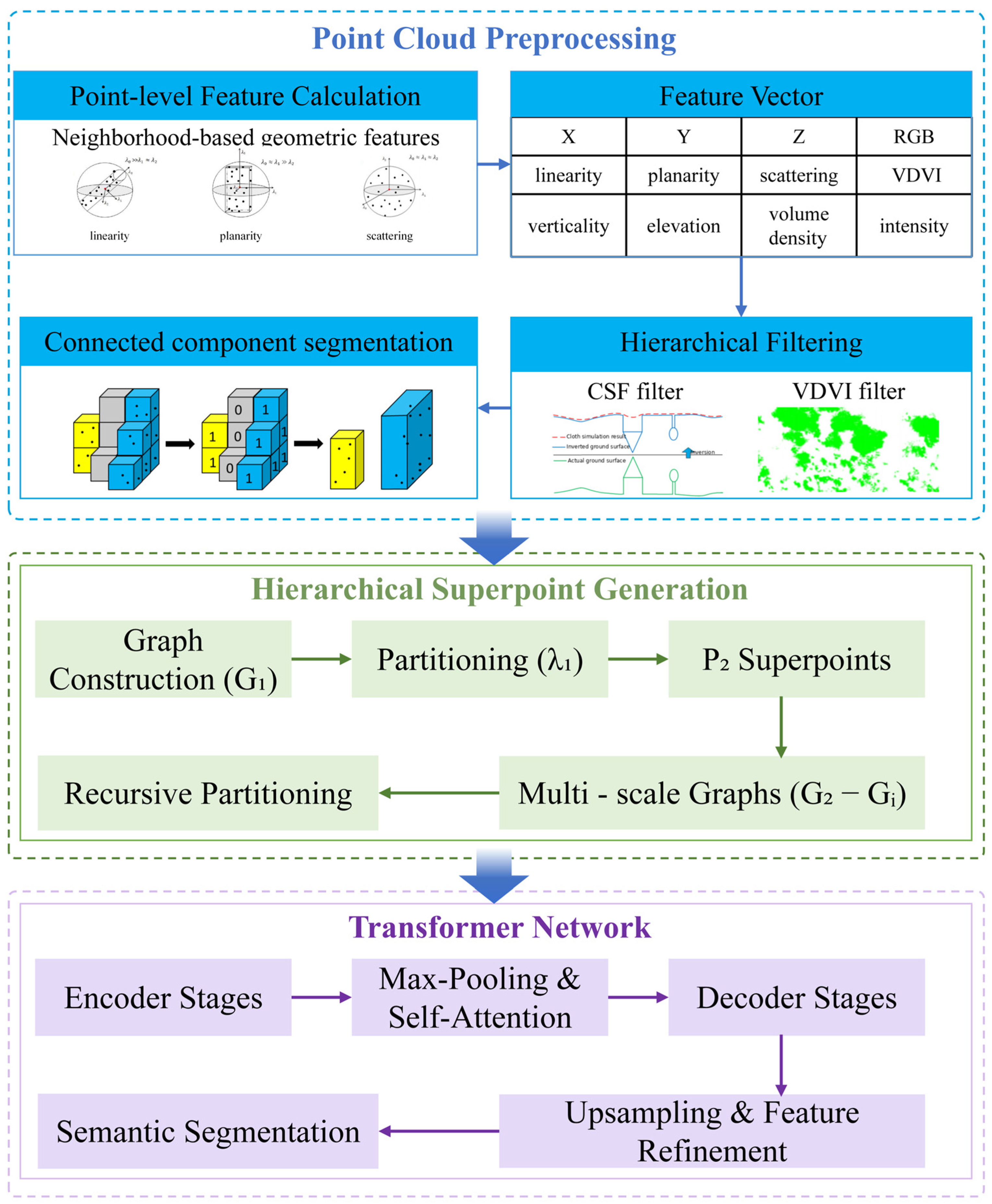
The ISPT algorithm integrates three key enhancements into the original SPT framework while preserving its hierarchical superpoint structure and transformer-based architecture (Figure 4). The workflow begins with point-level feature calculation, including geometric and radiometric features such as linearity, planarity, scattering, verticality, elevation, volumetric density, RGB, VDVI, and intensity.
Then, the hierarchical filtering first applies the Cloth Simulation Filter (CSF) to separate ground points from overhangs, followed by vegetation removal using VDVI thresholds (VDVI > 0.05). Next, connected component segmentation generates preliminary superpoints (P1) via voxel-based clustering. These P1 superpoints serve as the foundation for hierarchical superpoints generation, where iterative graph-based partitioning (J(e;f,G,λ)) recursively produces coarser partitions (P2, …, Pi) by balancing feature fidelity and geometric simplicity.
The superpoint graph construction builds adjacency graphs (G1, …, Gi) encoding centroid proximity and interface statistics. The transformer network processes these graphs with encoder–decoder stages: encoders aggregate features via max-pooling and self-attention, while decoders refine features by propagating contextual information from coarser levels. Self-attention mechanisms incorporate handcrafted adjacency features (e.g., centroid offset, pose) and learned keys/queries/values.
Finally, semantic segmentation outputs labels for P1 using a dual loss: cross-entropy for dominant labels at P1 and label distribution supervision for coarser levels to enforce hierarchical context learning. This integration of feature augmentation, hierarchical filtering, and connected component segmentation enhances discriminability and computational efficiency, enabling robust semantic analysis of complex vegetated terrains while retaining the original SPT’s compactness and scalability.

2.4. Recognition and Parameter Extraction of Rock Mass Discontinuity

Classified rock points are subjected to region-growing segmentation and least-squares plane fitting [42]. Structural attributes such as dip, dip direction, and trace length are computed for each planar surface. These parameters provide quantitative inputs for geotechnical stability analysis and hazard prediction.
The region-growing segmentation algorithm operates by iteratively expanding seed points based on normal vector consistency and curvature variations. Specifically, a KNN (K-Nearest Neighbors) neighborhood with 30 points is established to calculate normal vectors, and a threshold of 10° is applied to ensure planar continuity.
For each segmented plane, a local coordinate system is constructed by aligning the Z-axis with the plane’s normal vector derived from the least squares plane fitting equation:
a 0 x + a 1 y + a 2 z + a 3 = 0
where a0, a1, a2, and a3 are plane parameters, and a0, a1, and a2 cannot be zero at the same time. The plane normal vector n is (a0, a1, a2).
The calculation formula for the occurrence parameters of structural planes is as follows:
D d i r e c t i o n = arctan a 1 a 0
D a n g l e = arctan ( a 0 2 + a 1 2 a 2 )
where D d i r e c t i o n is the dip direction of the structural plane, and D a n g l e is the dip angle of the structural plane.
Points within the plane are then projected onto this local coordinate system to generate a grayscale intensity image, where pixel values correspond to point density and geometric features. The CannyLines operator is subsequently applied to detect 2D edge segments in the image, which are then back-projected into 3D space to identify discontinuity traces.

2.5. Accuracy Validation

2.5.1. Reconstruction Accuracy and Model Quality Validation

In addition to semantic segmentation accuracy, the geometric accuracy and quality of the photogrammetric 3D reconstruction were evaluated to ensure the reliability of the derived point cloud for subsequent vegetation filtering and discontinuity extraction. Following common practice in close-range UAV photogrammetry, the assessment focused on (i) georeferencing (absolute) accuracy using control/checkpoints, (ii) relative geometric accuracy using distance-consistency checks, and (iii) intrinsic point-cloud quality in terms of surface noise, completeness, and point density.
(i)
Georeferencing accuracy
Ground control points (GCPs) were used to georeference the reconstruction, while independent checkpoints were reserved for external validation. For each point i , coordinate residuals were computed as Δ X i = X i e s t X i r e f , Δ Y i = Y i e s t Y i r e f , and Δ Z i = Z i e s t Z i r e f . The root-mean-square error (RMSE) in each direction was then calculated as R M S E X = 1 n i = 1 n ( Δ X i ) 2 , R M S E Y = 1 n i = 1 n ( Δ Y i ) 2 , and R M S E Z = 1 n i = 1 n ( Δ Z i ) 2 , where n is the number of evaluated points. A planimetric RMSE was reported as R M S E X Y = R M S E X 2 + R M S E Y 2 , and the overall 3D RMSE was reported as follows:
R M S E 3 D = R M S E X 2 + R M S E Y 2 + R M S E Z 2
(ii)
Relative geometric accuracy
To quantify relative geometric fidelity after georeferencing, a set of m reference distances was established using selected point pairs with known separation. For each pair k, the distance measured in the reconstructed point cloud was computed as d k m o d e l = ( X a X b ) 2 + ( Y a Y b ) 2 + ( Z a Z b ) 2 and compared with the corresponding reference value d k r e f . Distance errors were defined as Δ d k = d k m o d e l d k r e f . The distance RMSE was then computed as follows:
R M S E d = 1 m k = 1 m ( Δ d k ) 2
The mean relative error was reported as
M R E = 1 m k = 1 m | Δ d k | d k r e f × 100 %
The selected distance pairs were distributed across the study area and spanned multiple orientations and scales to reduce potential bias.
(iii)
Point-cloud quality
Intrinsic quality of the reconstructed point cloud was evaluated by characterizing surface noise (local roughness), spatial completeness, and point density. Local roughness was quantified by fitting a plane to each point’s neighborhood and computing orthogonal point-to-plane distances r i ; the neighborhood roughness was summarized by an RMS statistic σ = 1 k i = 1 k r i 2 , where k is the neighborhood size. Completeness was evaluated by projecting the point cloud onto a local reference plane within the region of interest (ROI), discretizing it into a regular grid, and computing the proportion of grid cells whose point density exceeded a minimum threshold τ :
C = N c e l l s ( ρ τ ) N c e l l s , t o t a l × 100 %
where ρ denotes point density per grid cell. Overall point density was reported as ρ = N A , where N is the number of points within the ROI, and A is the corresponding projected area. Together, these measures provide complementary evidence that the photogrammetric reconstruction is geometrically reliable and sufficiently complete for downstream analysis.

2.5.2. Classification Accuracy Validation

In this paper, the accuracy evaluation method employs standard metrics including IoU (Intersection over Union), mACC (mean Accuracy), mIoU (mean Intersection over Union), and OA (Overall Accuracy).
For IoU, the calculation formula is as follows:
I o U = A B A B
where A represents the predicted result, and B denotes the actual result, measuring the overlap degree between predictions and actual outcomes for each category.
mACC (mean Accuracy) is derived by averaging the per-class accuracy values. For each class i, the accuracy is calculated as follows:
A C C i = T P i T P i + F N i
where TPi and FNi are the true positives and false negatives for class i. The mACC is then the arithmetic mean of these values across all classes.
OA (Overall Accuracy) is computed as the ratio of correctly predicted samples to the total number of samples:
O A = i = 1 C T P i T o t a l S a m p l e s
where C is the number of classes. This metric directly quantifies the model’s overall prediction correctness.
mIoU (mean Intersection over Union) aggregates the IoU values for all categories, providing an average measure of overlap consistency. Collectively, these metrics offer a multi-dimensional assessment of the model’s performance, ensuring comprehensive accuracy validation.

3. Results

3.1. The SPT Model Training

The SPT model was trained using a dataset consisting of labeled point clouds from the UAV survey. An NVIDIA GeForce RTX 4080 GPU was utilized for data training. The information on the training datasets is shown in Table 2, and the training parameters are presented in Table 3.

3.2. Reconstruction Accuracy and Model Quality Results

The reconstructed models’ accuracy and quality were assessed using three key indicators: (i) absolute georeferencing accuracy, (ii) relative geometric accuracy, and (iii) point-cloud quality metrics. This evaluation was conducted at each of the four test sites using ground control points. Overall, the results demonstrate centimeter-level accuracy in georeferencing and excellent model quality across all sites.
(i)
Georeferencing Accuracy
The absolute accuracy of each 3D model was quantified by the RMSE of ground control point (GCP) and check point residuals in horizontal (XY) and vertical (Z) dimensions. All four site models achieved horizontal RMSE on the order of only a few centimeters (≈2–5 cm), while vertical RMSE ranged from ~3 cm up to ~8 cm. The combined three-dimensional RMSE (spatial error) varied between approximately 4 cm for the most accurate reconstruction and ~9 cm for the least. For instance, Site3 exhibited the highest georeferencing accuracy, with RMSE_XY ≈ 2.3 cm and RMSE_Z ≈ 3.4 cm (yielding a 3D RMSE ~4.1 cm). In contrast, Site4 showed the largest residual errors (RMSE_XY ≈ 4.8 cm, RMSE_Z ≈ 7.5 cm, 3D RMSE ~8.9 cm). These differences can be attributed to factors such as the number and spatial distribution of GCPs and the complexity of the terrain at each site. Overall, the absolute positioning errors of ~2–5 cm horizontally and ~3–8 cm vertically are consistent with literature values for close-range UAV photogrammetry using GCPs.
(ii)
Relative Geometric Accuracy
The relative (internal) geometric accuracy of the models was evaluated by comparing known reference distances on the slope faces (e.g., between independent checkpoints or other surveyed features) to the corresponding distances measured in the 3D point clouds. All sites yielded very small discrepancies, indicating excellent preservation of scale and shape in the reconstructions. The distance measurement errors (distance residuals) were on the order of only 1–3 cm. In quantitative terms, the relative distance RMSE ranged from about 1.3 cm (Site3) to 2.8 cm (Site4), with the other sites falling in between (~1.7–2.3 cm). These low relative errors (well below 3 cm) demonstrate that the models’ internal geometry is highly accurate. In other words, distances and dimensions in the photogrammetric models closely match real-world values, with only a few centimeters of uncertainty over scales of several meters. This level of internal consistency gives confidence that no significant deformations or scale errors were introduced during the reconstruction.
(iii)
Point-Cloud Quality
Detailed point-cloud metrics further confirm the high fidelity of the UAV reconstructions. Surface roughness (local model noise) was low for all sites, on the order of ~1–2 cm. Here, roughness is quantified as the average deviation of points from local best-fit surfaces (indicating noise in flat areas). The smoothest model was produced at Site3, which had an average roughness of only ~1.0 cm, reflecting minimal noise on planar surfaces. The highest roughness was observed at Site4 (~1.9 cm), likely due to more complex surface geometry or minor vegetation on the slope face introducing noise. Even this worst-case noise level (~2 cm) is quite low given the high resolution of the data. The coverage ratio (model completeness) was also very high. Each site’s point cloud covered over 90% of the target slope surface area, despite the steep oblique imaging geometry. Site3 achieved the highest coverage at ~98%, indicating nearly the entire slope face was reconstructed, whereas Site4 had the lowest coverage at about 90% (suggesting only small portions of the surface were missed, likely due to occlusions or insufficient overlap).
Finally, the point clouds were extremely dense thanks to the close-range, high-overlap imaging strategy. The average point density ranged from roughly 820 to 1100 points/m2 across the sites. Site3 again had the densest cloud (~1100 pts/m2), benefitting from the short camera-to-target distance (3–4 m) and multiple flight passes that greatly increased overlap. Even the lowest density, at Site4 (~820 pts/m2), far exceeds the typical densities from standard nadir UAV surveys (often tens of pts/m2) and provides detailed coverage of the slope geometry. Such high point densities, combined with the high coverage and low noise, indicate that the oblique close-range UAV photogrammetry approach captured a nearly complete and very detailed 3D representation of each site. Table 4 summarizes the quantitative accuracy and quality results for all four sites, highlighting the consistency and differences in the metrics discussed above.

3.3. Vegetation and Rock Mass Classification Results

The proposed ISPT framework was evaluated on UAV-derived point clouds collected from four vegetated high-slope sites.
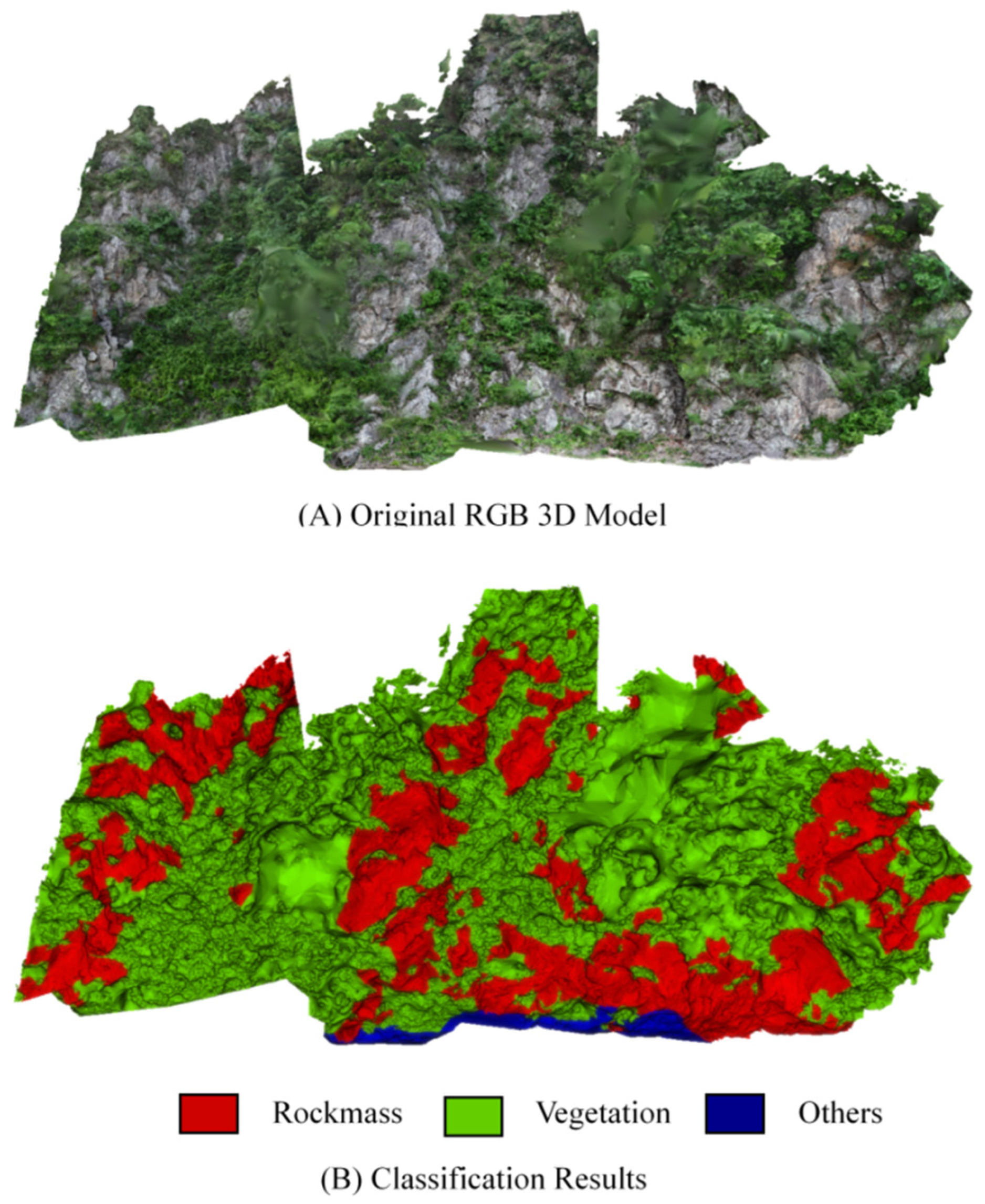
Figure 5 depicts a schematic illustration of the classification results for rock mass and vegetation point clouds of the test set. As shown in Figure 5B, the classification scheme partitions the scene into three distinct categories: rock mass (red), vegetation (green), and others (blue). Within the classified model, vegetation dominates, manifesting as extensive and contiguous green regions that signify its widespread distribution across the slope under investigation. Rock mass is delineated as discrete red patches, closely coinciding with the exposed rocky outcrops evident in the original RGB 3D model (Figure 5A). Visual inspection confirmed that the proposed approach generated clean segmentation boundaries and accurately delineated structural planes, even in areas partially covered by dense vegetation. Figures illustrate classification maps, segmentation outputs, and histograms of extracted parameters.
Table 5 presents the updated classification accuracy evaluation results of the test set. For the Intersection over Union (IoU) metric, the “Vegetation” class exhibits an IoU score of 63.8, indicating moderate overlap between predicted and actual vegetation regions. This may be attributed to the complex morphological variability and occlusions inherent in natural vegetation canopies, which challenge the algorithm’s boundary discrimination. The “Rock” class achieves a notably higher IoU of 88.4, reflecting robust classification performance likely due to the more stable geometric characteristics and less dynamic spatial distribution of rock mass compared to vegetation.
The mean accuracy (mACC) stands at 72.5, quantifying the average proportion of correctly classified points across all classes, while the mean IoU (mIoU) is 76.1, providing a class-balanced measure of overlap quality. These metrics collectively indicate consistent cross-class performance, with the model demonstrating stronger discriminative ability for rock mass than vegetation. The overall accuracy (OA) is 89.5, which confirms the robustness of ISPT in distinguishing rock surfaces from vegetation under challenging occlusion conditions.
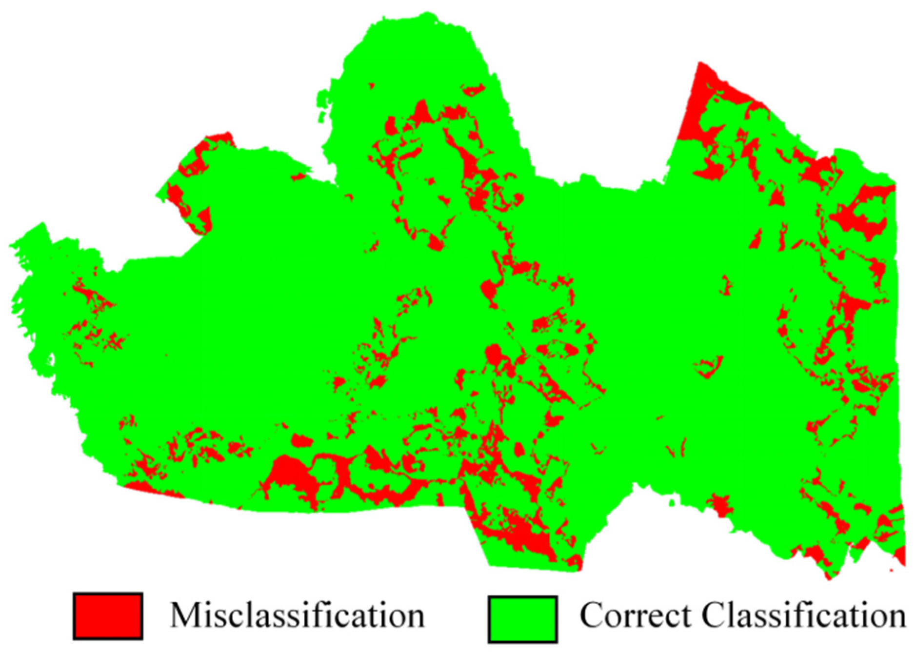
Figure 6 shows the classification errors in the classification results of the test set. By analyzing these errors, we can further understand the limitations of the algorithm. Misclassifications may occur due to various factors. For example, the similarity in appearance between some rocks and vegetation under certain lighting conditions or the presence of small-scale geological features that are difficult to distinguish can lead to misclassifications. In addition, the resolution of the UAV-captured images and the complexity of the natural terrain also play important roles.

3.4. Recognition Results of Planar Surfaces in Rock Mass

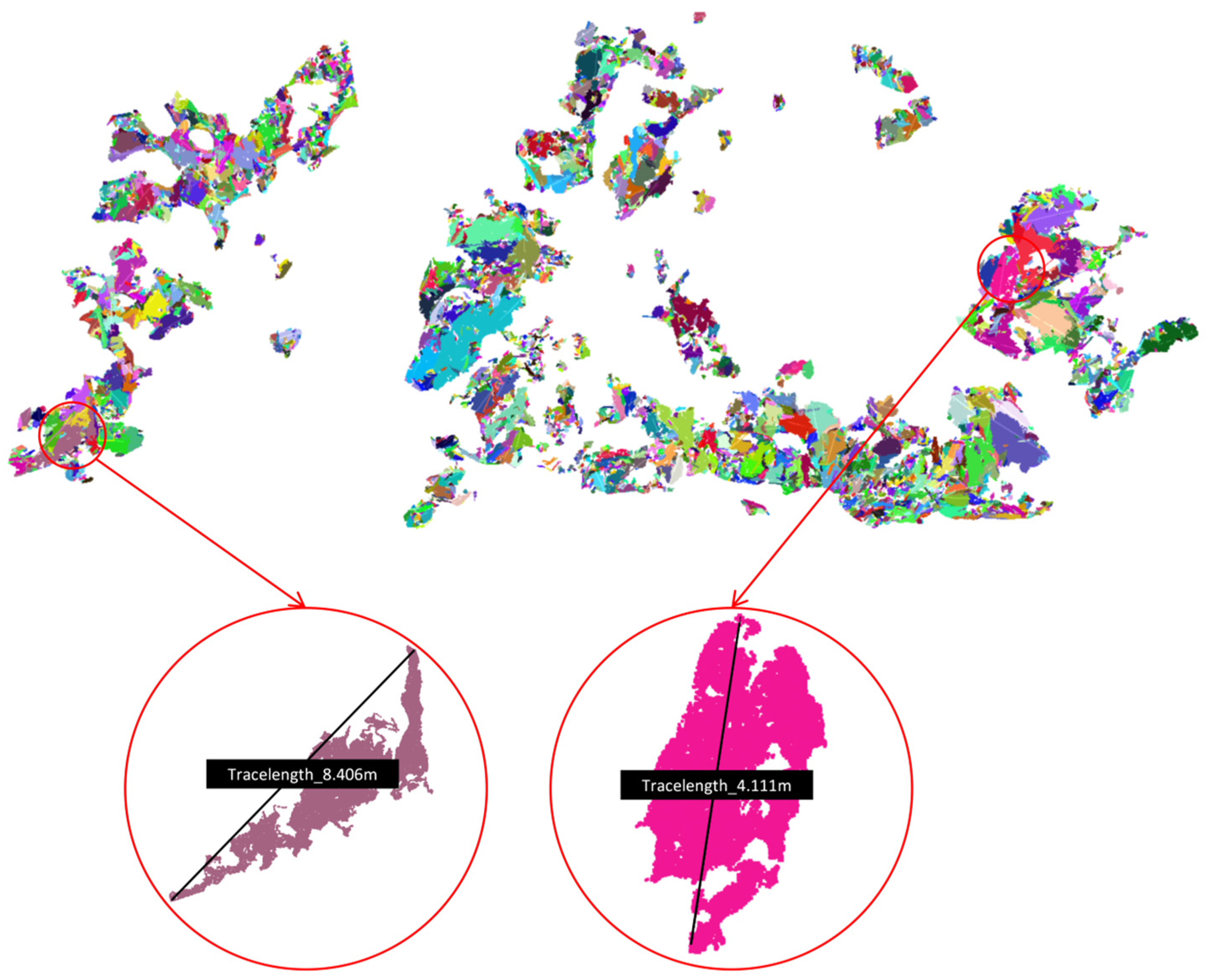
According to the method described in Section 2.4, the classified rock mass point clouds were used for the identification of planar surfaces in the rock mass. In the test set, a total of 4918 planar surfaces were extracted. Figure 7 shows the plane segmentation results of the rock mass surface. Each planar point cloud is randomly colored for distinction. The local enlarged image in the red frame demonstrates two rock mass planar point clouds and their trace lengths.

3.5. Rock Mass Structural Parameters Extraction Results

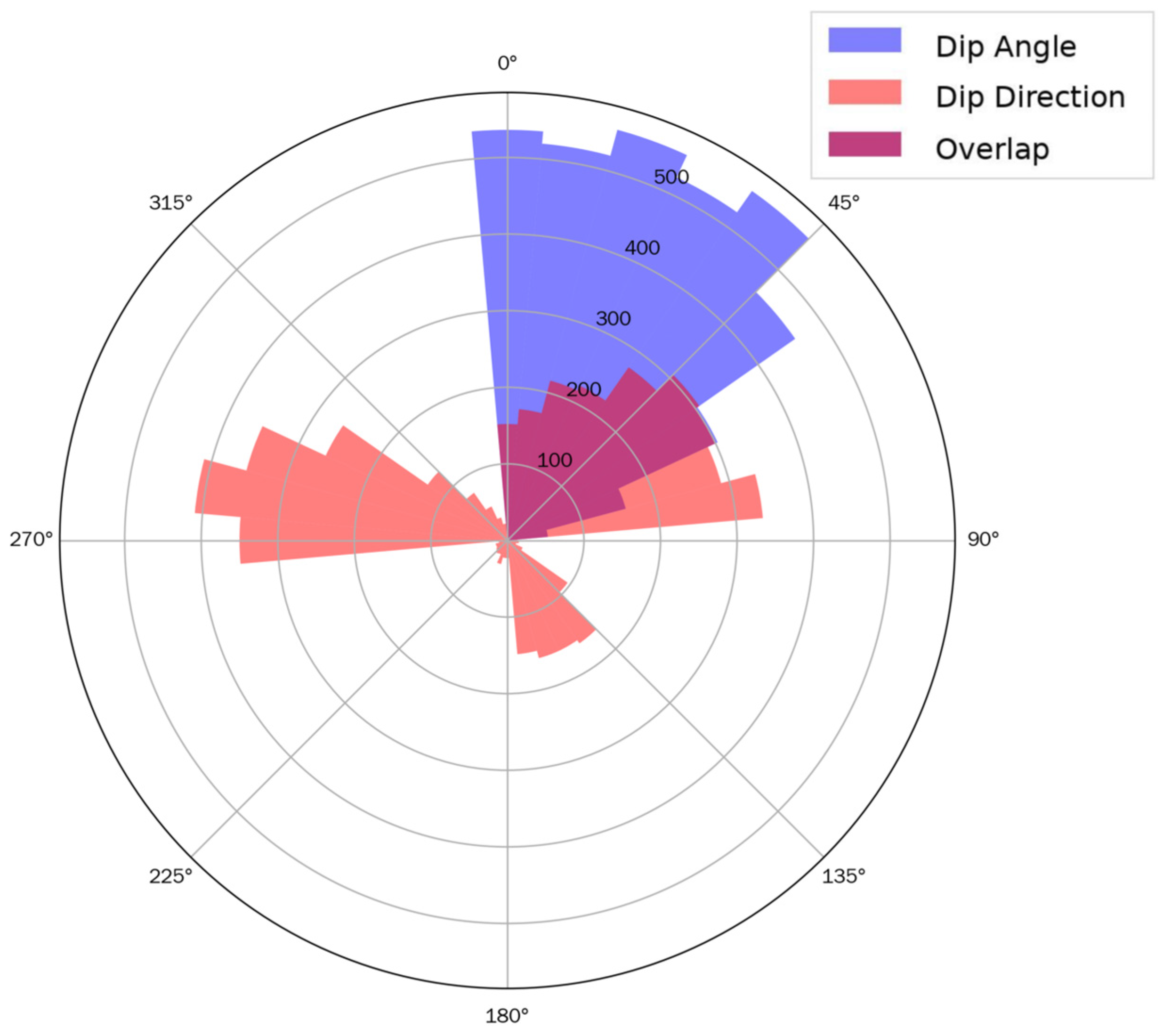
The datasets contain 4918 data points characterizing rock mass planes with three parameters: dip angle (in degrees), azimuth orientation (in degrees), and trace length (in meters). Figure 8 presents histograms of these parameters, illustrating their distribution patterns:
Dip angle ranges from −46.00° to 88.00°, with a prominent peak around 22.00° (the median), indicating a preferred inclination. The distribution spreads symmetrically from this peak toward both extremes, with fewer data points at the boundaries, reflecting significant variability in dip angles likely caused by tectonic forces and erosion.
Azimuth orientation spans 0.00° to 359.00° and exhibits a multimodal distribution, featuring main peaks at 141.00° (median) and 282.00° (75th percentile). This suggests multiple dominant azimuthal directions of rock mass planes, possibly resulting from distinct phases of geological stress during rock mass formation and deformation.
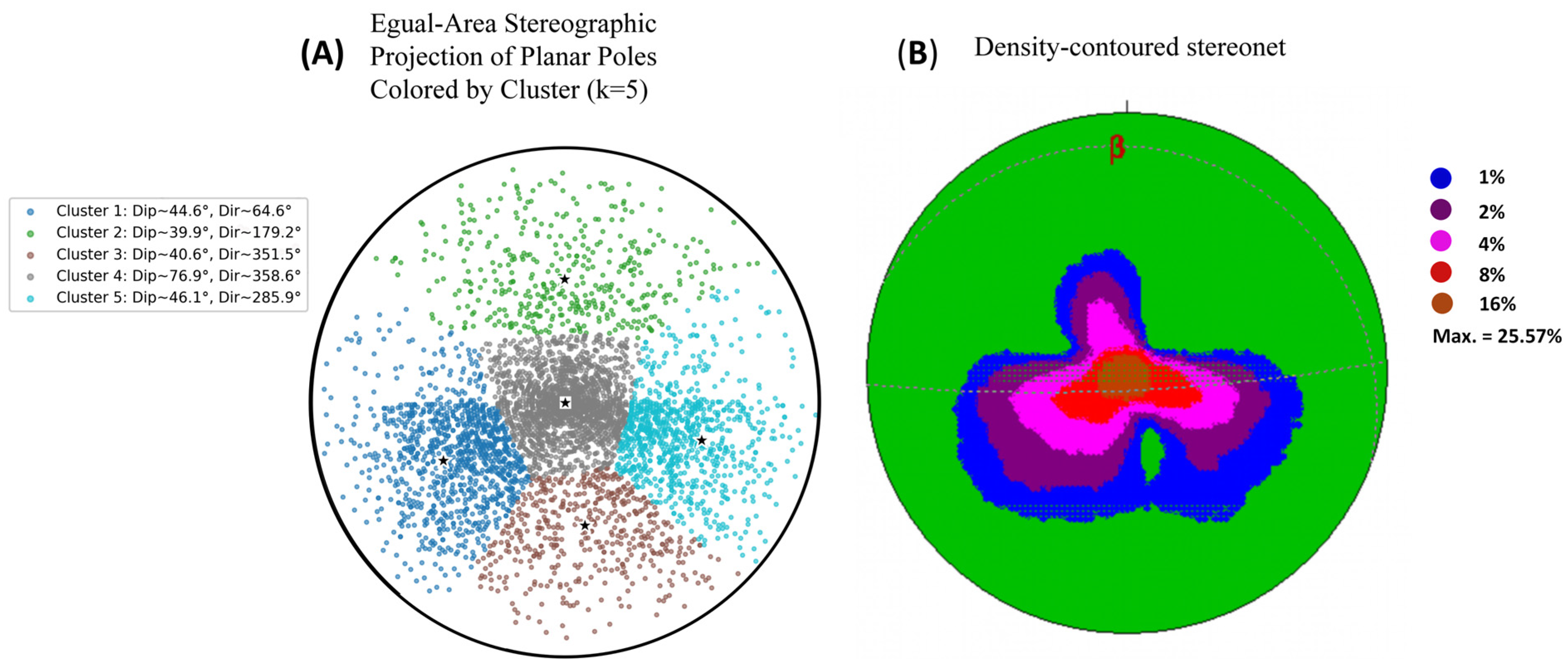
To perform clustering on the spherical domain, the 3D orientation of each discontinuity plane was converted to its pole (normal vector). By representing the pole orientations as three-dimensional direction cosine vectors, the K-means clustering algorithm was applied, and the optimal number of clusters (k) was determined using the silhouette coefficient within the range of 2–6. The results indicated that the silhouette coefficient reached its maximum at k = 5, which was therefore adopted to define five joint sets (Table 6).
An equal-area stereographic projection was employed to map each pole onto the unit circle, with the projection radius r defined as a function of the complementary angle of the dip d as follows:
r = 2 sin ( d 2 )
Figure 9 illustrates the stereographic projection of the five clusters. Different colors represent distinct discontinuity sets, and the stars denote the centroid of each cluster, corresponding to the mean geometric parameters. A contoured gridded density plot was generated to visually represent the distribution of geological orientation data via grids and contour lines, aiming to highlight the concentration of such data and facilitate the identification of dominant orientations, distribution patterns, and key features. The contoured grid density plot in panel (B) exhibits a maximum density of 25.57%, with contour gradients depicting the spatial variability of pole concentrations. Quantitative orientation analysis reveals a mean principal orientation of 8°/20°, a mean resultant direction of 8–017°, and a mean resultant length of 0.82 (variance = 0.18), indicating a moderately concentrated distribution of planar data. Additionally, the calculated girdle (82°/177°) and beta axis (8–357°) imply the presence of cylindrical folding, where the beta axis approximates the fold hinge orientation.
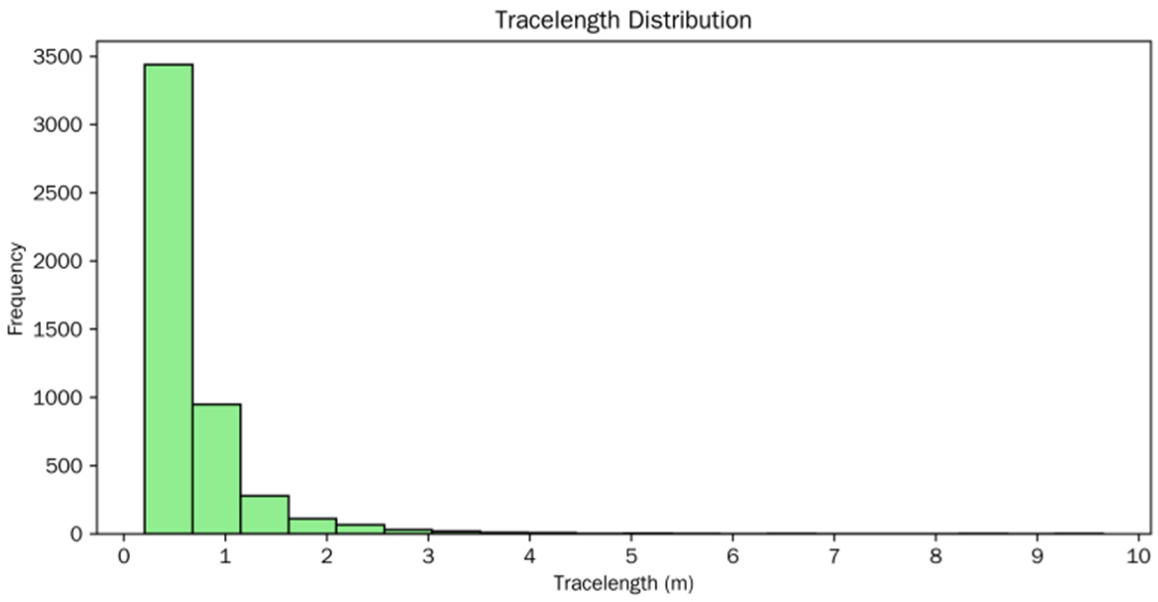
This study extracted the trace length of individual geological planes. Trace length varies from 0.20 m to 9.65 m, with data concentrated at the lower end. The distribution peaks at 0.51 m (median) and tapers off with increasing trace length, where the majority of values fall below 0.75 m (75th percentile). The long-tailed distribution toward higher values indicates occasional occurrences of significantly longer trace lengths, potentially associated with specific geological events or rock properties promoting extensive fracturing (Figure 10).

4. Discussion

The experimental results underscore the effectiveness of ISPT in overcoming two major limitations of UAV-based rock mass analysis: vegetation occlusion and computational inefficiency. By integrating VDVI-based filtering and volumetric density features, ISPT significantly improved vegetation removal compared to purely geometric or radiometric methods. Furthermore, the hierarchical partitioning strategy and connected-component pre-segmentation enabled efficient processing of large-scale point clouds without compromising accuracy.

4.1. Comparisons

To compare the differences in accuracy and efficiency between the method proposed in this study and traditional machine learning algorithms, and to verify the improvement effect on the SPT algorithm, we conducted a comparative analysis with the natural scene point cloud classification algorithm based on multi-scale geometric features (CANUPO) proposed by Brodu et al. and the original SPT algorithm [43]. CANUPO, which employs multi-scale geometric features based on Principal Component Analysis (PCA), is representative among algorithms using neighborhood geometric features for point cloud classification. Compared with other algorithms that only use single-scale or dual-scale features, it is expected to yield higher and more stable classification results. Additionally, this algorithm is based on machine learning supervised classification, making it representative among many such branch-leaf separation algorithms. Furthermore, it provides a free and open-source application, facilitating comparative analysis.
The CANUPO algorithm consists of three main steps: (1) extraction of multi-scale neighborhood geometric features, where the size and number of neighborhoods can be freely set according to requirements. A larger number of neighborhoods increases the computational load but can improve classification accuracy to a certain extent; (2) sample selection and training; (3) point-by-point classification based on multi-scale Support Vector Machine (SVM). Currently, this algorithm provides a free, open-source program suite. Additionally, the algorithm is integrated as a plugin into CloudCompare for greater usability. In this study, the CANUPO plugin in CloudCompare was used for algorithm comparison: http://www.cloudcompare.org/doc/wiki/index.php?title=CANUPO_(plugin) (accessed on 2 August 2025).
In the experiments, to achieve the optimal classification performance of CANUPO and ensure the objectivity and reliability of the results, we selected the required training samples for CANUPO from the manually classified training set. When extracting multi-neighborhood geometric features, the neighborhood sizes were set to ten scales ranging from 0.02 m to 0.32 m. Based on the geometric features of these ten scales, the Balance Accuracy (BAcc) of the training samples were 91.5%, 98.2%, and 90.6%, respectively, and the Fisher Discriminant Ratios (FDRs) were 5.38, 6.94, and 5.24, respectively, indicating that the selection of neighborhood sizes and quantities can achieve optimal classification results.
The results show that the algorithm (ISPT) proposed in this study significantly outperforms the CANUPO algorithm in accuracy and slightly surpasses the original SPT algorithm. The overall classification accuracy of the proposed algorithm is 89.5%, while that of the CANUPO algorithm is 78.2%, and the original SPT algorithm is 85.8%, as shown in Table 7. Compared to the CANUPO algorithm, ISPT achieved higher accuracy and reduced execution time by an order of magnitude. While traditional methods rely heavily on handcrafted geometric descriptors, ISPT leverages feature-rich representations and self-attention mechanisms to capture both local and global context. These findings align with emerging trends in point cloud analysis, where transformer-based models increasingly replace conventional approaches for semantic segmentation tasks.
In this study, the reported desktop configuration was used for the deep learning-based point-cloud processing of the proposed workflow. The primary hardware specifications were: Intel Core i7-8700 CPU (3.20 GHz), 32 GB RAM, and NVIDIA GeForce RTX 4080 GPU. The total execution times for the three algorithms are presented in Table 8. It should be noted that the reported times exclude data I/O operations, parameter tuning, sample selection, and model training durations. Efficiency analysis demonstrated that ISPT reduced computational time to 6.52 min compared to 164.28 min for CANUPO, representing a 25× improvement in processing speed (Table 8). The extraction stage successfully identified 4918 planar surfaces with calculated geometric parameters: dip angles ranged from −46° to 88°, azimuth orientations exhibited multimodal distributions, and trace lengths varied from 0.2 m to 9.65 m. These quantitative metrics are critical for downstream geotechnical stability assessment.

4.2. Advantages

UAV photogrammetry enables high-resolution topographic data acquisition from inaccessible or hazardous slopes (e.g., high-steep cliffs). By capturing multi-angle imagery at centimeter-scale resolution, it generates dense 3D point clouds and digital surface models (DSMs) that facilitate millimeter- to centimeter-scale fracture mapping. The limitations of UAVs include their relatively weak endurance (limited battery life), which restricts the duration of field data acquisition. Although professional UAV platforms and mission-planning software can support pre-programmed flights, close-range oblique imaging of hazardous, near-vertical slopes often requires manual adjustments to maintain safe stand-off distances and avoid occlusions, making the achieved overlap less controllable than in standard nadir surveys. This necessitates manual control of the UAV during shooting, making quantitative control of the image overlap ratio difficult to achieve.
The advantages of deep learning algorithms lie in their good adaptability to complex environments and complex rock mass structures [44]. In this study, deep learning algorithms achieved higher accuracy than traditional machine learning algorithms. Through hierarchical feature extraction capabilities, deep learning models can effectively capture the nonlinear relationships in rock mass structures (such as the spatial topology of fracture networks and the local variations in lithological textures) [45], thereby achieving more accurate identification in complex geological environments.
Furthermore, due to the adoption of the Super Point Segmentation (SPS) strategy, the deep learning model used in this study can achieve fast segmentation of large-volume point clouds, with a multiple-fold speed improvement compared to traditional machine learning algorithms. The SPS strategy replaces point-by-point calculations with semantic clustering, addressing the computational bottleneck of traditional algorithms in processing large-volume point clouds.

5. Conclusions

This study presents an automated and efficient framework for rock mass discontinuity recognition on vegetated high slopes by combining UAV photogrammetry and an Improved Superpoint Transformer. The proposed ISPT model integrates VDVI-based vegetation filtering, volumetric density features, hierarchical segmentation, and transformer-based self-attention, resulting in superior classification accuracy (89.5%) and computational efficiency (25× faster than traditional methods). The ability to extract thousands of structural planes with quantified parameters underscores its practical value for geotechnical hazard assessment and slope stability analysis.

Author Contributions

Conceptualization, P.W.; Methodology, P.W.; Software, P.W. and R.Z.; Validation, X.H.; Formal analysis, P.W. and X.H.; Data curation, P.W.; Writing—original draft, P.W.; Writing—review & editing, X.H., R.Z. and X.G.; Supervision, X.G.; Project administration, X.G.; Funding acquisition, X.H. All authors have read and agreed to the published version of the manuscript.

Funding

This work was supported by the National Natural Science Foundation of China (Grant Nos. 42271447 and 42001374) and, in part, by the Fundamental Research Funds for Central Public Welfare Research Institutes (Grant Nos. CKSF2021449/GC and CKSF2025705/GC).

Data Availability Statement

The original contributions presented in this study are included in the article. Further inquiries can be directed to the corresponding author.

Conflicts of Interest

The authors declare no conflict of interest.

References

  1. Hudson, J.A.; Priest, S.D. Discontinuities and Rock Mass Geometry. Int. J. Rock Mech. Min. Sci. Geomech. Abstr. 1979, 16, 339–362. [Google Scholar] [CrossRef]
  2. Zhang, W.; Zhao, Q.; Huang, R.; Chen, J.; Xue, Y.; Xu, P. Identification of Structural Domains Considering the Size Effect of Rock Mass Discontinuities: A Case Study of an Underground Excavation in Baihetan Dam, China. Tunn. Undergr. Space Technol. 2016, 51, 75–83. [Google Scholar] [CrossRef]
  3. Sharma, V.M.; Saxena, K.R. (Eds.) In-Situ Characterization of Rocks; A. A. Balkema Publishers: Leiden, The Netherlands, 2001. [Google Scholar]
  4. Li, H.; Li, X.; Li, W.; Zhang, S.; Zhou, J. Quantitative Assessment for the Rockfall Hazard in a Post-Earthquake High Rock Slope Using Terrestrial Laser Scanning. Eng. Geol. 2019, 248, 1–13. [Google Scholar] [CrossRef]
  5. Cirillo, D.; Zappa, M.; Tangari, A.C.; Brozzetti, F.; Ietto, F. Rockfall Analysis from UAV-Based Photogrammetry and 3D Models of a Cliff Area. Drones 2024, 8, 31. [Google Scholar] [CrossRef]
  6. Lovitt, J.; Rahman, M.; McDermid, G. Assessing the Value of UAV Photogrammetry for Characterizing Terrain in Complex Peatlands. Remote Sens. 2017, 9, 715. [Google Scholar] [CrossRef]
  7. Mao, Z.; Hu, S.; Wang, N.; Long, Y. Precision Evaluation and Fusion of Topographic Data Based on UAVs and TLS Surveys of a Loess Landslide. Front. Earth Sci. 2021, 9, 801293. [Google Scholar] [CrossRef]
  8. Han, X.; Yang, S.; Zhou, F.; Wang, J.; Zhou, D. An Effective Approach for Rock Mass Discontinuity Extraction Based on Terrestrial LiDAR Scanning 3D Point Clouds. IEEE Access 2017, 5, 26734–26742. [Google Scholar] [CrossRef]
  9. Liang, H.; Xiao, J.; Ying, W. A Vegetation Filtering Method for Rock Mass Point Clouds Based on Multi-Dimensionality Features and MLP. J. Univ. Chin. Acad. Sci. 2020, 37, 345–351. [Google Scholar]
  10. Kong, X.; Xia, Y.; Wu, X.; Wang, Z.; Yang, K.; Yan, M.; Li, C.; Tai, H. Discontinuity Recognition and Information Extraction of High and Steep Cliff Rock Mass Based on Multi-Source Data Fusion. Appl. Sci. 2022, 12, 11258. [Google Scholar] [CrossRef]
  11. Wang, Y.; Xu, S.; Xiao, J.; Wang, F.; Wang, Y.; Liu, L. Accurate Rock-Mass Extraction From Terrestrial Laser Point Clouds via Multiscale and Multiview Convolutional Feature Representation. IEEE Trans. Geosci. Remote Sens. 2021, 59, 4430–4443. [Google Scholar] [CrossRef]
  12. Hussain, Y.; Schlögel, R.; Innocenti, A.; Hamza, O.; Iannucci, R.; Martino, S.; Havenith, H.-B. Review on the Geophysical and UAV-Based Methods Applied to Landslides. Remote Sens. 2022, 14, 4564. [Google Scholar] [CrossRef]
  13. Westoby, M.J.; Brasington, J.; Glasser, N.F.; Hambrey, M.J.; Reynolds, J.M. ‘Structure-from-Motion’ Photogrammetry: A Low-Cost, Effective Tool for Geoscience Applications. Geomorphology 2012, 179, 300–314. [Google Scholar] [CrossRef]
  14. Hao, J.; Zhang, X.; Wang, C.; Wang, H.; Wang, H. Application of UAV Digital Photogrammetry in Geological Investigation and Stability Evaluation of High-Steep Mine Rock Slope. Drones 2023, 7, 198. [Google Scholar] [CrossRef]
  15. Drews, T.; Miernik, G.; Anders, K.; Höfle, B.; Profe, J.; Emmerich, A.; Bechstädt, T. Validation of Fracture Data Recognition in Rock Masses by Automated Plane Detection in 3D Point Clouds. Int. J. Rock Mech. Min. Sci. 2018, 109, 19–31. [Google Scholar] [CrossRef]
  16. Chen, B.; Maurer, J.; Gong, W. Applications of UAV in Landslide Research: A Review. Landslides 2025, 22, 3029–3048. [Google Scholar] [CrossRef]
  17. Yang Bisheng, D.Z. Progress and Perspective of Point Cloud Intelligence. Acta Geod. Sin. 2019, 48, 1575–1585. [Google Scholar]
  18. Hartwig, M.E.; Santos, G.G.D.S.D. Enhanced Discontinuity Mapping of Rock Slopes Exhibiting Distinct Structural Frameworks Using Digital Photogrammetry and UAV Imagery. Environ. Earth Sci. 2024, 83, 624. [Google Scholar] [CrossRef]
  19. Yang, L.; Li, Y.; Li, X.; Meng, Z.; Luo, H. Efficient Plane Extraction Using Normal Estimation and RANSAC from 3D Point Cloud. Comput. Stand. Interfaces 2022, 82, 103608. [Google Scholar] [CrossRef]
  20. Pola, A.; Herrera-Díaz, A.; Tinoco-Martínez, S.R.; Macias, J.L.; Soto-Rodríguez, A.N.; Soto-Herrera, A.M.; Sereno, H.; Ramón Avellán, D. Rock Characterization, UAV Photogrammetry and Use of Algorithms of Machine Learning as Tools in Mapping Discontinuities and Characterizing Rock Masses in Acoculco Caldera Complex. Bull. Eng. Geol. Environ. 2024, 83, 260. [Google Scholar] [CrossRef]
  21. Wu, S.; Wang, Q.; Zeng, Q.; Zhang, Y.; Shao, Y.; Deng, F.; Liu, Y.; Wei, W. Automatic Extraction of Outcrop Cavity Based on a Multiscale Regional Convolution Neural Network. Comput. Geosci. 2022, 160, 105038. [Google Scholar] [CrossRef]
  22. Oppikofer, T.; Jaboyedoff, M.; Pedrazzini, A.; Derron, M.; Blikra, L.H. Detailed DEM Analysis of a Rockslide Scar to Characterize the Basal Sliding Surface of Active Rockslides. J. Geophys. Res. Earth Surf. 2011, 116, F02016. [Google Scholar] [CrossRef]
  23. Xu, Q.; Ye, Z.; Liu, Q.; Dong, X.; Li, W.; Fang, S.; Guo, C. 3D Rock Structure Digital Characterization Using Airborne LiDAR and Unmanned Aerial Vehicle Techniques for Stability Analysis of a Blocky Rock Mass Slope. Remote Sens. 2022, 14, 3044. [Google Scholar] [CrossRef]
  24. Štroner, M.; Urban, R.; Suk, T. Filtering Green Vegetation Out from Colored Point Clouds of Rocky Terrains Based on Various Vegetation Indices: Comparison of Simple Statistical Methods, Support Vector Machine, and Neural Network. Remote Sens. 2023, 15, 3254. [Google Scholar] [CrossRef]
  25. Anders, N.; Valente, J.; Masselink, R.; Keesstra, S. Comparing Filtering Techniques for Removing Vegetation from UAV-Based Photogrammetric Point Clouds. Drones 2019, 3, 61. [Google Scholar] [CrossRef]
  26. Wernette, P.A. Machine Learning Vegetation Filtering of Coastal Cliff and Bluff Point Clouds. Remote Sens. 2024, 16, 2169. [Google Scholar] [CrossRef]
  27. Wang, Y.; Koo, K.-Y. Vegetation Removal on 3D Point Cloud Reconstruction of Cut-Slopes Using U-Net. Appl. Sci. 2021, 12, 395. [Google Scholar] [CrossRef]
  28. Blanco, L.; García-Sellés, D.; Guinau, M.; Zoumpekas, T.; Puig, A.; Salamó, M.; Gratacós, O.; Muñoz, J.A.; Janeras, M.; Pedraza, O. Machine Learning-Based Rockfalls Detection with 3D Point Clouds, Example in the Montserrat Massif (Spain). Remote Sensing 2022, 14, 4306. [Google Scholar] [CrossRef]
  29. Pinto, M.F.; Melo, A.G.; Honório, L.M.; Marcato, A.L.M.; Conceição, A.G.S.; Timotheo, A.O. Deep Learning Applied to Vegetation Identification and Removal Using Multidimensional Aerial Data. Sensors 2020, 20, 6187. [Google Scholar] [CrossRef]
  30. Fan, Z.; Wei, J.; Zhang, R.; Zhang, W. Tree Species Classification Based on PointNet++ and Airborne Laser Survey Point Cloud Data Enhancement. Forests 2023, 14, 1246. [Google Scholar] [CrossRef]
  31. Han, X.; Liu, C.; Zhou, Y.; Tan, K.; Dong, Z.; Yang, B. WHU-Urban3D: An Urban Scene LiDAR Point Cloud Dataset for Semantic Instance Segmentation. ISPRS J. Photogramm. Remote Sens. 2024, 209, 500–513. [Google Scholar] [CrossRef]
  32. Vivaldi, V.; Bordoni, M.; Mineo, S.; Crozi, M.; Pappalardo, G.; Meisina, C. Airborne Combined Photogrammetry—Infrared Thermography Applied to Landslide Remote Monitoring. Landslides 2023, 20, 297–313. [Google Scholar] [CrossRef]
  33. Kalinicheva, E.; Landrieu, L.; Mallet, C.; Chehata, N. Predicting Vegetation Stratum Occupancy from Airborne LiDAR Data with Deep Learning 2022. Int. J. Appl. Earth Obs. Geoinf. 2022, 112, 102863. [Google Scholar] [CrossRef]
  34. Diab, A.; Kashef, R.; Shaker, A. Deep Learning for LiDAR Point Cloud Classification in Remote Sensing. Sensors 2022, 22, 7868. [Google Scholar] [CrossRef] [PubMed]
  35. Šašak, J.; Gallay, M.; Kaňuk, J.; Hofierka, J.; Minár, J. Combined Use of Terrestrial Laser Scanning and UAV Photogrammetry in Mapping Alpine Terrain. Remote Sens. 2019, 11, 2154. [Google Scholar] [CrossRef]
  36. Salvini, R.; Vanneschi, C.; Coggan, J.S.; Mastrorocco, G. Evaluation of the Use of UAV Photogrammetry for Rock Discontinuity Roughness Characterization. Rock Mech. Rock Eng. 2020, 53, 3699–3720. [Google Scholar] [CrossRef]
  37. Chen, K.; Jiang, Q. Discontinuity Surface Orientation Extraction and Cluster Analysis Based on Point Cloud Data. Can. Geotech. J. 2025, 62, 1–9. [Google Scholar] [CrossRef]
  38. Zhu, J.; Xia, Y.; Wang, B.; Yang, Z.; Yang, K. Research on the Identification of Rock Mass Structural Planes and Extraction of Dominant Orientations Based on 3D Point Cloud. Appl. Sci. 2024, 14, 9985. [Google Scholar] [CrossRef]
  39. Robert, D.; Raguet, H.; Landrieu, L. Efficient 3D Semantic Segmentation with Superpoint Transformer. In Proceedings of the 2023 IEEE/CVF International Conference on Computer Vision (ICCV), Paris, France, 1–6 October 2023; IEEE: New York, NY, USA, 2023; pp. 17149–17158. [Google Scholar]
  40. Wang, X.; Wang, M.; Wang, S.; Wu, Y. Extraction of Vegetation Information from Visible Unmanned Aerial Vehicle Images. Trans. Chin. Soc. Agric. Eng. (Trans. CSAE) 2015, 31, 152–159. [Google Scholar] [CrossRef]
  41. Zhang, W.; Qi, J.; Wan, P.; Wang, H.; Xie, D.; Wang, X.; Yan, G. An Easy-to-Use Airborne LiDAR Data Filtering Method Based on Cloth Simulation. Remote Sens. 2016, 8, 501. [Google Scholar] [CrossRef]
  42. Wang, X.; Zou, L.; Shen, X.; Ren, Y.; Qin, Y. A Region-Growing Approach for Automatic Outcrop Fracture Extraction from a Three-Dimensional Point Cloud. Comput. Geosci. 2017, 99, 100–106. [Google Scholar] [CrossRef]
  43. Brodu, N.; Lague, D. 3D Terrestrial Lidar Data Classification of Complex Natural Scenes Using a Multi-Scale Dimensionality Criterion: Applications in Geomorphology. ISPRS J. Photogramm. Remote Sens. 2012, 68, 121–134. [Google Scholar] [CrossRef]
  44. Yu, H.; Taleghani, A.D.; Al Balushi, F.; Wang, H. Machine Learning for Rock Mechanics Problems; an Insight. Front. Mech. Eng. 2022, 8, 1003170. [Google Scholar] [CrossRef]
  45. Han, X.; Chen, X.; Deng, H.; Wan, P.; Li, J. Point Cloud Deep Learning Network Based on Local Domain Multi-Level Feature. Appl. Sci. 2023, 13, 10804. [Google Scholar] [CrossRef]
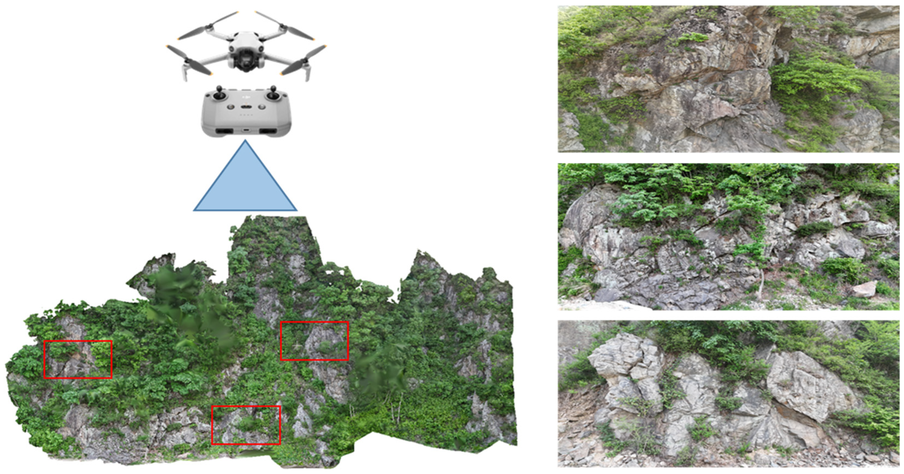
Figure 1. Close-up images of the high-slope rock mass in Study Area 4. The red rectangles in the reconstructed model delineate the regions of interest, whose spatial extents correspond to the close-up views shown in the right-hand panels.
Remotesensing 18 00357 g001
Figure 2. The overall workflow of this study.
Remotesensing 18 00357 g002
Figure 3. The three-dimensional reconstruction results of the four study areas in this study.
Remotesensing 18 00357 g003
Figure 4. The overall workflow of the improved SPT algorithm.
Remotesensing 18 00357 g004
Figure 5. Schematic diagram of the classification results of rock mass and vegetation point clouds.
Remotesensing 18 00357 g005
Figure 6. Classification errors in the classification results.
Remotesensing 18 00357 g006
Figure 7. Plane segmentation results of the rock mass surface and their trace lengths. The point-cloud colors are randomly assigned, and each distinct color denotes the points belonging to an individual planar segment.
Remotesensing 18 00357 g007
Figure 8. Rose diagram of dip angle and dip direction. “Overlap” denotes the angular range where the dip-angle and dip-direction distributions overlap.
Remotesensing 18 00357 g008
Figure 9. An equal-area stereographic projection (A) and the contoured grid density plot (B). In plot (A), the black five-pointed stars indicate the cluster centroids. In plot (B), β denotes the dip direction (azimuth) of the reference plane.
Remotesensing 18 00357 g009
Figure 10. Histogram distributions of trace length.
Remotesensing 18 00357 g010
Table 1. Summary of representative studies.
Authors
(Year)
TechniquesAdvantagesDisadvantagesApplication
Scenarios
Pola et al. (2024) [20]UAV photogrammetry + k-means on normals + RANSACMaps multiple discontinuity sets remotely; uses free 3D toolsRelies on quality of point cloud; requires manual ROI removal pre- stepLarge inaccessible caldera outcrops
Šašak et al. (2019) [35]SfM photogrammetry, TLS/ALS comparisonHigh-res DTMs/DOMs; easy deployment; low cost for steep cliffsNo direct dense cloud; vegetation occlusion; lower absolute accuracy than TLSCoastal cliff rockfall assessment; geomorphology
Salvini et al. (2020) [36]UAV-SfM point cloud vs. field/TLS validationUAV point clouds can reliably capture joint roughness (>60 cm scales)Less accurate for very short profiles (<60 cm); requires multiple flight heightsQuantitative joint roughness analysis
Chen et al. (2025) [37]PCA normals + Hough + region-growing + DBSCANRobust normal estimation (Hough); clusters planes automatically; widely citedSensitive to point density and noise; complex parameter tuningAlgorithmic plane extraction from TLS/photogrammetry clouds
Zhu et al. (2024) [38]Hough transform + CFSFDP clusteringAutomates the number of planes; robust normal at edges; handles large slopesComputationally intensive; accuracy depends on voting parameters; memory heavyHighway slope joint mapping; engineering geology
Wang et al. (2021) [27]2D image segmentation (U-Net) + 3D reprojection (point cloud)Effectively removes vegetation for change detection; uses proven CNN models Requires labeled training data; 2D segmentation errors project to 3DTime-series monitoring of vegetated cut slopes
Fan et al. (2023) [30]PointNet++ deep networkEnd-to-end learning of point features; high accuracy (~92%)Data-hungry; requires downsampling or augmentation; slow to trainTree species and vegetation classification from LiDAR
Table 2. Training datasets of the SPT.
Dataset ClassificationData SamplesPoint Cloud Quantity
Training SetSite1-117,428,162
Site1-217,143,557
Site2-15,498,532
Site2-212,190,668
Validation SetSite3-11,187,707
Site3-210,889,558
Test SetSite4-19,178,136
Site4-27,863,002
Table 3. Training parameters of SPT.
ParametersValue
Batch size1
Epoch500
Parameters of Superpoint SegmentationVoxel Size: 0.03
KNN: 30
Number of Point Feature Samples within Superpoints:
[Sample_point_min: 32; Sample_point_max: 128]
Point features used for trainingRGB, VDVI, Linearity, Curvature, Planarity, Scattering, Verticality, Elevation, Volumetric density.
Horizontal edge features used for training(1) ‘mean_off’; (2) ‘std_off’; (3) ‘mean_dist’; (4) ‘angle_source’; (5) ‘angle_target’; (6) ‘centroid_dir’; (7) ‘centroid_dist’; (8) ‘normal_angle’; (9) ‘log_length’; (10) ‘log_surface’; (11) ‘log_volume’; (12) ‘log_size’
Table 4. Reconstruction accuracy and point-cloud quality metrics for the four test sites.
MetricSite1Site2Site3Site4
Horizontal RMSE (XY) [cm]2.93.72.34.8
Vertical RMSE (Z) [cm]4.563.47.5
3D RMSE [cm]5.474.18.9
Relative distance RMSE [cm]1.72.31.32.8
Surface roughness [cm]1.31.611.9
Coverage ratio [%]95939890
Point density [pts/m2]9508701100820
Table 5. Evaluation results of classification accuracy.
Accuracy MetricsClassAccuracy Score
IoUVegetation63.8
Rock88.4
mACC 72.5
mIoU 76.1
OA 89.5
Table 6. Summary of clustered discontinuity sets.
Cluster IDMean Dip Angle (°)Mean Dip Direction (°)Sample Count (n)
144.664.6 (ENE)1045
239.9179.2 (S)407
340.6351.5 (NNW)480
476.9358.6 (N)2103
546.1285.9 (WNW)883
Note: Mean dip angle and mean dip direction represent the average orientation of the discontinuity planes in each cluster. Sample count (n) indicates the number of planes assigned to each cluster.
Table 7. Comparison of classification accuracies among the proposed ISPT algorithm, CANUPO, and original SPT algorithm.
MethodsAccuracy MetricsAccuracy Score
ISPT (proposed method)mACC72.5
mIoU76.1
OA89.5
CANUPOmACC63.3
mIoU66.5
OA78.2
Original SPTmACC69.5
mIoU73
OA85.8
Table 8. Runtime comparison of ISPT, CANUPO, and baseline SPT.
MethodsTime-Consuming (min)
ISPT (proposed method)6.52
CANUPO164.28
Original SPT5.21
Disclaimer/Publisher’s Note: The statements, opinions and data contained in all publications are solely those of the individual author(s) and contributor(s) and not of MDPI and/or the editor(s). MDPI and/or the editor(s) disclaim responsibility for any injury to people or property resulting from any ideas, methods, instructions or products referred to in the content.