Highlights
What are the main findings?
- A residual U-Net convolutional neural network trained on PlanetScope imagery (~4.77 m) accurately mapped canopy openings across 1761 km2, achieving 92.2% overall accuracy and an F1-score of 95.1%, with independent LiDAR validation confirming operational performance (85.9% accuracy, F1-score 0.77) across diverse terrain.
- Alaska Peak fuel reduction treatments (2020–2024) created 564 acres of new openings, increasing structural heterogeneity, with 56% of open area within 12 m of residual canopy. However, the large openings (>5 acres) slightly exceeded historical reference conditions for the region.
What are the implications of the main findings?
- This validated deep learning workflow provides forest managers with a scalable, cost-effective monitoring framework to rapidly evaluate restoration treatment effectiveness using commercially available satellite imagery, bridging the gap between expensive LiDAR and coarse-resolution products.
- The framework enables adaptive management by revealing treatment outcomes in actionable metrics; while Alaska Peak treatments successfully fragmented dense canopy and created beneficial edge habitat, refinements to thinning prescriptions could better align opening size distributions with historical reference conditions.
Abstract
Forest management interventions in fire-prone western U.S. forests aim to restore structural heterogeneity, yet tracking treatment efficacy at landscape scales remains a persistent challenge. Traditional monitoring tools often lack the spatial resolution or temporal frequency needed to assess fine-scale structural outcomes. While deep learning approaches for mapping canopy structure from high-resolution satellite imagery have advanced rapidly, their application to operational monitoring of restoration outcomes with independent validation remains limited. This study demonstrates and validates a scalable monitoring workflow that integrates high-resolution PlanetScope multispectral imagery (~4.77 m) with a residual U-Net convolutional neural network (CNN) to quantify canopy structure dynamics in support of forest restoration programs. Trained using 3 m canopy cover data from the California Forest Observatory (CFO) as a reference, the model accurately segmented forest canopy from openings across a large, independent test area of ~1761 km2, with an overall accuracy of 92.2%, and an F1-score of 95.1%. Independent validation against airborne LiDAR across 140 km2 of heterogeneous terrain confirmed operational performance (overall accuracy 85.9%, F1-score 0.77 for canopy gaps). We applied this framework to quantify structural changes within the North Yuba Collaborative Forest Landscape Restoration Program from 2020 to 2024, providing managers with actionable metrics to evaluate treatment effectiveness against historical reference conditions. The treatments created 564 acres of new openings, significantly increasing structural heterogeneity, with 56% of new open area located within 12 m of residual canopy. While treatment outcomes aligned with the goal of fragmenting dense canopy, the resulting large openings (>5 acres) slightly exceeded historical reference conditions for the area. This validated workflow translates high-resolution satellite imagery into timely, actionable metrics of forest structure, enabling managers to rapidly evaluate treatment impacts and refine restoration strategies in fire-prone ecosystems.
1. Introduction
The increasing severity and scale of disturbances, particularly wildfires, are reshaping western United States dry forests. Extended droughts, rising temperatures, and a legacy of fire suppression have left these ecosystems densely overgrown and highly vulnerable to stand-replacing fires [1,2]. In response, proactive forest management now emphasizes fuels reduction treatments, including mechanical thinning and prescribed burning, to reduce fuel loads and improve forest resilience [3,4]. One goal of these treatments is to restore structural heterogeneity by creating fine-grained mosaics of tree clumps, canopy openings, and individual trees characteristic of historical, frequent-fire regimes [1,5,6,7]. Assessing whether these efforts achieve their intended spatial patterns requires reliable monitoring methods capable of measuring changes in forest structure at high resolution across vast and often remote landscapes.
Meeting this monitoring need is complicated by the difficulty of capturing fine-scale canopy structures at landscape scales, which directly influence fire behavior and restoration success [5,8,9]. Traditional field surveys are spatially limited, while moderate resolution satellites like Landsat (30 m) cannot resolve the individual tree crowns or small canopy openings (50.1 ha) that are ecologically significant [10,11]. Even medium-resolution satellites, such as Sentinel-2 (~10 m), lack the fine resolution required to detect small-scale canopy openings relevant to ecological processes. While airborne LiDAR can delineate these features with sub-meter precision [6,12,13], its high cost remains a barrier for more frequent, landscape-scale monitoring required by adaptive management frameworks. Additionally, curated datasets of canopy cover metrics are often delayed by months or years, limiting the ability of forest managers to act quickly [9,11]. Given these challenges, there is a growing need for moderate-to-high resolution, adaptable monitoring tools that can capture changes in forest structure with both precision and frequency across large landscapes [8,11].
Commercial satellite constellations such as PlanetScope (~3–5 m resolution, daily revisit) bridge this spatiotemporal gap. The <5 m resolution of PlanetScope imagery provides an optimal scale for forest monitoring, as individual pixels begin to approximate the dimensions of single tree crowns (~6 m; [14]), while maintaining the landscape-wide coverage necessary for regional analysis [8,9]. Deep learning methods, particularly convolutional neural networks (CNNs), have proven effective for mapping forest structure from such imagery. Recent studies have successfully applied CNNs with PlanetScope and similar high-resolution platforms to detect individual trees, map forest cover, and monitor deforestation [15,16,17,18,19], yet targeted applications to restoration monitoring remain limited. Translating this wealth of high-resolution imagery into validated and actionable ecological metrics for forest managers presents a significant analytical challenge. Operational use requires robust validation against independent datasets, classification schemes aligned with management frameworks, and scalable processing workflows [8,9,20].
We address that operational gap by developing and independently validating a workflow that enables land managers to evaluate fine-scale restoration outcomes using commercially available satellite imagery. Our objectives were to: (1) develop and train a CNN-based model to accurately detect canopy openings from PlanetScope imagery; (2) independently validate model performance across extensive spatial scales (~1760 km2) using high-resolution airborne LiDAR (~140 km2) to ensure reliability across heterogeneous landscapes; (3) demonstrate operational utility by quantifying how thinning treatments change canopy structure compared to management objectives based on historical reference conditions. This workflow provides forest managers with a validated, scalable pathway to monitor canopy structural changes and support adaptive management in fire-prone ecosystems [8].
2. Methods
2.1. Study Region
The study was conducted within the 978,381-hectare Tahoe-Central Sierra Initiative (TCSI) partnership landscape in the Central Sierra Nevada of California, USA (approx. 39°22′54.8”N 120°32′58.7”W). The region spans an elevation gradient from approximately 1500 to 8000 feet (450 to 2440 m). The landscape is dominated by Sierra mixed-conifer forest, comprised primarily of ponderosa pine (Pinus ponderosa), white fir (Abies concolor), incense cedar (Calocedrus decurrens), Douglas-fir (Pseudotsuga menziesii), and sugar pine (Pinus lambertiana), with oak woodlands at lower elevations and red fir (Abies magnifica), whitebark pine (Pinus albicaulis), and Western white pine (Pinus monticola) at higher elevations [21]. The TCSI landscape was selected due to the partnership’s focus on large-landscape forest restoration aimed at improving forest ecosystem and community resilience to severe wildfires, drought, beetle-related mortality, and climate change [22].
Our analysis follows a multi-scale hierarchy (Figure 1). The deep learning model was developed and validated for the entire TCSI landscape. We then applied the validated model to conduct a detailed case study within the ~275,000 ha North Yuba Landscape Resilience Project [23], a Collaborative Forest Landscape Restoration Program (CFLRP) project and designated Wildfire Crisis Strategy landscape located within the TCSI. The case study focuses specifically on quantifying treatment outcomes within the 504 ha Alaska Peak Project, where mechanical thinning occurred between 2020 and 2024 (see Text S1, Alaska Peak Project and treatment context).
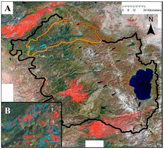
Figure 1.
Map of detected canopy changes (2020–2024) based on multispectral PlanetScope imagery and a CNN model across the TCSI (Tahoe-Central Sierra Initiative) landscape. Both panels show Planetscope RGB imagery from the third quarter of 2023. Pixel-level changes in canopy cover between 2020–2024 are denoted in red (canopy loss) and bright green (canopy gain). In Panel (A), the black outline denotes the TSCI landscape boundary, the orange outline represents the North Yuba CFLRP, and the cyan polygons show the Alaska Peak project area. Major areas of canopy loss (in red), moving north to south, occur along the southern edge of the North Complex Fire (2020), the Mosquito Fire (2022), and the Caldor Fire (2021). Panel (B) provides an inset showing the Alaska Peak Project. Canopy loss and gain predictions applied within a 20-mile buffer of the TCSI landscape. RGB imagery shown is from 2023 as this processed visual product was only available for that year, while the 8-band multispectral imagery was used for all quantitative analyses (2020–2024). The resolution of pixels is 4.77 m.
2.2. Satellite Imagery and Reference Data
2.2.1. PlanetScope Imagery
We used PlanetScope 8-band quarterly analysis-ready mosaics (Planet Basemaps, Surface Reflectance) with a spatial resolution of 4.77 m. This spatial resolution provides a useful scale to measure canopy cover changes, as 1 pixels is approximately equivalent to the 6 m threshold distance used to identify clumps of conifer trees with interlocking crowns, or within one crown width of each other [13,14]. This resolution bridges the gap between coarse-resolution satellites that miss fine-scale features and expensive and processing heavy LiDAR acquisitions. It provides sufficient detail to detect management-induced structural changes while maintaining the temporal frequency and spatial coverage needed for adaptive management.
We specifically accessed the Level 3B products that are orthorectified (<10 m RMSE) and include radiometric corrections [24]. We used the third quarter (July–September) mosaics for training the model, because they are spectrally normalized to Sentinel-2 observations to minimize sensor-to-sensor variation. The eight spectral bands included were: coastal blue (431–452 nm), blue (465–515 nm), green I (513–549 nm), green (547–583 nm), yellow (600–620 nm), red (650–680 nm), red-edge (697–713 nm), and near-infrared (NIR; 845–885 nm). The year 2020 was chosen because it is the only year where freely available California Forest Observatory (CFO) canopy cover metrics, which served as the reference dataset for model training, overlap with the Planet 8-band surface reflectance imagery (see Text S2, data processing).
Planet Basemap imagery was accessed and downloaded using the Planet Basemaps API via Python. Briefly, we used the API to download the ‘quads’ associated with the TCSI region (including a 10-mile buffer). In total, this buffered TCSI region was split across 105 quads. Each of the 105 quads is 4096 × 4096 pixels (16,777,216 pixels per quad), for a total of 80.04 km2 (19,779.4 acres) per quad.
2.2.2. Reference Data for Model Training
Training a deep learning model for robust, landscape-scale application requires a spatially extensive and consistent training dataset that traditional field plots cannot provide. We leveraged the California Forest Observatory’s (CFO) 3 m canopy cover product as a high-quality proxy for ground truth. The CFO’s metrics are derived from high-precision airborne LiDAR data and then scaled statewide using deep learning and satellite imagery. The underlying CFO models were validated against an independent LiDAR dataset (>15,000 km2), explaining 91% of the variance in canopy cover (r2 = 0.91) with a mean absolute error of 7.0% [25]. This ‘wall-to-wall’ reference dataset allows the model to learn from a vast and diverse range of forest conditions, a prerequisite for reaching the generalization necessary for regional monitoring. The high, validated accuracy of the CFO canopy cover product provides a strong foundation for training our classification model and has been used in several recent studies [26,27,28,29,30]. The 2020 CFO data for 2020 were accessed using the CFO-public Google Cloud Bucket (LINK).
Before transforming the canopy cover data, we used bilinear interpolation in ArcGIS Pro (v3.2) to match the resolution of the 3 m CFO canopy cover product to the resolution of the ~4.77 m PlanetScope imagery. Because our focus is not on the percentage of canopy cover per pixel, but instead on identifying pixels that shift from canopy to non-canopy class (i.e., newly formed openings), we next transformed the CFO canopy cover percentages into two categories. Pixels with >50% canopy cover were classified as “Forest”, whereas pixels with <50% canopy cover were classified as “non-forest.” This 50% threshold was selected to represent closed canopy forest conditions for several reasons. First, it aligns with commonly used definitions of “closed-canopy” forest in remote sensing (e.g., [31]), wherein areas above roughly half-coverage of canopy are considered tree-dominated. Second, it provides a clear, interpretable cutoff for distinguishing “forest” from more open conditions, ensuring that any appreciable drop in canopy closure (i.e., below 50%) would be detected as newly formed openings. Third, this binary split helps isolate meaningful changes in structure rather than small variations in canopy density that might not constitute functionally different conditions on the ground. Since the target class was forest openings, we labeled canopy cover pixels as zero and canopy opening pixels as one. The appropriateness of this binary classification approach was subsequently assessed through independent validation against airborne LiDAR (Section 2.5)
2.3. CNN Input Data Preparation
In total, 46 PlanetScope quads, covering 3681.84 km2 were used as input for model training and testing. The input for the CNN consisted of 15 data channels (Figure 2). In addition to the eight PlanetScope spectral bands, we calculated four spectral indices known to be sensitive to vegetation structure and health [32,33]. Normalized Difference Vegetation Index (NDVI), Normalized Difference Red Edge Index (NDRE), Green Normalized Difference Vegetation Index (GNDVI), and Visible Atmospherically Resistant Index (VARI) (equations in Text S2). Topographic features can influence vegetation patterns and help models account for terrain effects on canopy structure [34]. Therefore, we incorporated three topographic variables: elevation, slope, and aspect from NASA Shuttle Radar Topography Mission (SRTM) V3 digital elevation model (DEM) product (SRTMGL1_003) [35]. See Text S2: Extended data preparation & acquisition detail for additional information on processing of DEM data.
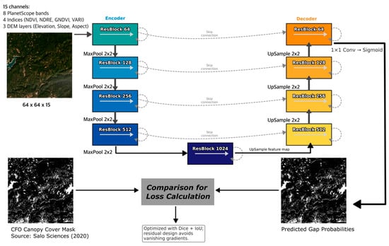
Figure 2.
Schematic of the U-Net-style convolutional neural network with residual blocks used for semantic segmentation of canopy openings. The input to the network is a 64 × 64 pixel tile with 15 channels (8 PlanetScope spectral bands, 4 derived spectral indices [NDVI, NDRE, GNDVI, VARI], and 3 DEM-derived topographic variables [elevation, slope, aspect]). In the encoder (left), successive Residual Blocks with 64, 128, 256, and 512 filters are each followed by 2 × 2 max-pooling to reduce spatial resolution. A bottleneck Residual Block with 1024 filters captures high-level features at the deepest layer. In the decoder (right), 2 × 2 upsampling layers precede Residual Blocks with 512, 256, 128, and 64 filters; at each decoder level, feature maps are concatenated with the corresponding encoder outputs via skip connections to recover fine-scale spatial context. A final 1 × 1 convolution and sigmoid activation produce the per-pixel probability of canopy opening.
Both the 15-channel input data and the binary CFO reference raster were tiled into 64 × 64 pixel patches for model training and validation. This relatively small tile size was chosen to allow the model to focus on localized features while also capturing enough context to distinguish between canopy openings and forested canopy [36]. Further, smaller tile sizes can reduce computational complexity and memory requirements while also making training and inference more efficient [37]. See Text S2: Extended data preparation & acquisition detail for additional preprocessing steps. We excluded 136 tiles and masks with no corresponding CFO canopy cover data. The image tiles and corresponding masks were divided into training and validation datasets using an 80/20 split.
2.4. CNN Architecture, Training, and Validation
2.4.1. Model Architecture
We implemented a U-Net style convolutional neural network with residual blocks to perform semantic segmentation of canopy openings [38]. The U-Net architecture excels at image segmentation tasks as it captures both local and global contextual information by combining features from different levels of the network. It does this by combining a downsampling encoder path to capture contextual features with an upsampling decoder path to recover precise spatial detail via skip connections.
In our model, the encoder part of the network consists of four convolutional layers, each containing two residual blocks followed by a max-pooling layer. The residual blocks facilitate training deeper networks by allowing gradients to flow directly through shortcut connections [39]. The decoder mirrors the encoder structure, using upsampling layers to recover spatial resolution and concatenating the corresponding encoder feature maps to improve localization accuracy [38].
We chose this architecture because U-Net models with residual connections have shown improved performance compared to standard U-Net architectures without residual connections, particularly in segmentation tasks where the amount of training data is limited [40]. The combination of U-Net’s strong localization capability, which allows for precise boundary detection, and the increased depth provided by residual blocks allows the model to effectively capture both fine-grained spatial details and high-level contextual abstractions [38,41] (see Text S3: Detailed CNN architecture & hyper-parameters for additional information on CNN model structure and parameter choices).
2.4.2. Model Training
We trained the model by developing a custom data generator that loads the tiles and masks on-the-fly, applies normalization, and performs data augmentation. The model was trained using the Adam optimizer [42], with an initial learning rate of 2 × 10⁻⁴. The Adam optimizer is effective for training deep neural networks due to its adaptive learning rate and momentum [43]. The binary cross-entropy loss function was used to optimize the model during training by comparing the predicted probabilities of each pixel being a canopy opening to the ground-truth labels from CFO canopy cover masks [44]. We also monitored accuracy, precision, recall, the Dice coefficient, and the Intersection over Union (IoU) to evaluate the model’s performance.
Training was performed using a batch size of 64 for a maximum of 100 epochs [43]. The U-Net CNN model was developed using the TensorFlow (v 2.12.0) and Keras (v 2.12.0) frameworks in Python [45,46]. See Text S3: Training hyper-parameters & software environment for information on model callbacks and additional software used in the modelling pipeline.
2.4.3. Model Performance and Validation
We evaluated the performance of the trained U-Net CNN model using an independent test set consisting of 22 quads covering 435,146.8 acres (~1761 km2) in the TCSI study region. A custom data generator was again used to manage the test dataset during evaluation. This generator loaded test tiles and masks on-the-fly, then normalized them using global means and standard deviations calculated across the entire data set during training. The test dataset generator did not include data augmentation or shuffling.
The model’s performance on the independent test set was quantified using the binary cross-entropy loss, accuracy, precision, recall, intersection over union (IoU), Dice coefficient, F1-score, and ROC-AUC (One-vs-Rest). A confusion matrix was calculated for the test set to quantify the model’s true positive, true negative, false positive, and false negative rates [38].
2.5. Independent Validation with Airborne LiDAR
To independently assess model accuracy beyond the CFO-based training data, we conducted validation using high-resolution airborne LiDAR from the U.S. Geological Survey 3D Elevation Program [47]. We used data from the CA_SierraNevada_B22 project meeting Quality Level 1 specifications (≥8 pts/m2, vertical accuracy 9.74 cm) collected November-December 2021. Specifically, we compared the 2021 third quarter PlanetScope predictions against the LiDAR data collected in late 2021. This comparison was particularly valuable as it also allowed us to assess the model’s temporal generalizability on imagery from a year outside of the 2020 training period.
The validation workflow used the lidR package [48] in R. Specifically, raw LiDAR point clouds were processed to create canopy height models. Ground points were classified using the Cloth Simulation Filter algorithm [49], which is effective in complex terrain. Point clouds were then normalized to height above ground using Triangular Irregular Network interpolation [50]. Finally, we generated 2 m resolution Canopy Height Models and classified pixels < 3 m as gaps, a threshold commonly applied for distinguishing canopy from low vegetation in conifer forests [51,52].
We used a window-based validation approach to address spatial misalignments observed between the PlanetScope-based predictions and the LiDAR reference data, a known challenge with multi-source remote sensing data (e.g., [16]). Specifically, we applied a 3 × 3 pixel spatial tolerance, where a classified pixel is considered correct if its label matches any of the corresponding pixels in the 8-pixel neighborhood [53]. This approach accounts for inherent positional uncertainties between datasets [54], without requiring manual re-registration. Finally, fire-affected tiles were excluded by identifying tiles that visually overlapped with burn area perimeters from the Monitoring Trends in Burn Severity (MTBS) dataset [55], as LiDAR measures dead standing trees as “canopy,” whereas our spectral model classifies them as gaps.
2.6. Case Study: Quantifying Canopy Change in Alaska Peak
The third goal of this study was to use the trained and validated model to evaluate the effectiveness of fuels reduction treatments on restoring forest canopy structure to reference conditions in the Alaska Peak area. To do this, we first created a mosaic of canopy and opening predictions across the TCSI landscape to the boundaries of the Alaska Peak treatment units. We excluded the surrounding landscape from downstream analyses to avoid quantifying changes that fall outside of treatment units. The resulting raster of canopy openings and canopy clumps were converted to polygons. Each polygon was then assigned a unique ID, and its area and perimeter were calculated in square meters.
We next classified the refined temporal maps of canopy openings and forest patches into size classes reflecting the Historical Range of Variability (HRV; hereafter referring to the pre-suppression reference conditions of forest structure), thereby aligning our analysis with management objectives aimed at restoring forest conditions within the Natural Range of Variability (NRV) [23,56]. These HRV bins-specifically 0–0.25 acres, 0.25–0.5 acres, 0.5–1.0 acres, 1–3 acres, 3–5 acres, and 5+ acres-have increasingly been adopted by the USDA Forest Service to characterize forest structure under resilient, historically fire-active regimes [23]. They provide a benchmark forest structure characteristic of resilient forests that include a complex mosaic of individual trees, clumps, and openings. For this size-class analysis, we used polygon-level statistics to calculate the total acreage and number of individual patches within each size class for both openings and forest patches, tracking changes through time. This approach yields insights into how effectively treatments shifted the distribution towards size classes characteristic of fire-resilient forests and created or maintained the desired mosaic of smaller openings and clumps indicative of enhanced forest resilience.
Previous studies have applied morphological opening operations, or have delineated canopy openings using tools such as PatchMorph, we chose to exclude this approach. See Text S4: Alaska Peak GIS & HRV-bin processing details for justification. Further, other LiDAR-based studies [5,6] have used slightly different minimum canopy opening sizes (e.g., 0.03 ac) and bin definitions. However, we chose to match the size classes used in treatment planning to match the local planning context, simplify communication about forest conditions, and facilitate adaptive management decisions within this landscape.
To compare the distribution of forest patch area and open canopy area, we obtained HRV data from the Northern Sierra Historical Range of Variability and Current Landscape Departure [56], a General Technical Report prepared for the USDA Forest Service. In the report, historical forest and opening patch sizes were reconstructed for subbasin-scale landscapes within the Upper Yuba watershed, which covers the CFLR project area (Figure 1), to estimate the range and distribution of conditions prior to modern management [56]. We extracted HRV records for forest patch area and open canopy area by size class across all subbasins within the Upper Yuba Watershed and used them as a baseline to compare current conditions.
When comparing our results to HRV, an important caveat to note is that the CNN canopy opening-detection model identifies openings purely from spectral evidence of absent canopy at ~5 m resolution, whereas the HRV data set classifies “open” conditions from developmental-stage attributes such as tree-height and cover thresholds applied at a coarser grain. Specifically, HRV defines openings using tree height < 4.5 ft and applies tree cover thresholds within 40 m radius neighborhoods, integrating both vertical structure and horizontal coverage at a much broader spatial scale than our pixel-level detection. Because the two approaches define and map openings differently, the comparison is best interpreted as a relative, rather than one-to-one, indication of departure from historical conditions. Nonetheless, the HRV comparison still provides a useful relative benchmark for historical departure.
2.7. Openings by Size Class
Forest clumps and openings were identified and analyzed using ArcGIS Pro (v3.2). The initial data consisted of raster predictions indicating forest canopy (pixel value = 0) and canopy openings (pixel value = 1) in each year. Openings were defined as areas at least one crown radius (~3 m) away from forest canopy pixel in all directions. Each opening polygon was classified by its area (m2).
A distance analysis was then conducted to characterize how far each open canopy pixel lay from canopy. The masked distance raster was reclassified into discrete distance bins ranging from 6–72 m, adapting from the approach in [13], thereby allowing for the categorization of openings by their distance from canopy. For each year, the total area and proportion of openings within each distance bin were summarized (see Text S4: Detailed GIS and R processing steps for opening-distance analysis).
2.8. Computing Environment
All models were trained on a 2023 MacBook Pro with Apple M2 Pro chip (12 cores: 8 performance, 4 efficiency) and 32 GB memory, demonstrating that the framework can be developed without specialized GPU infrastructure. Training time averaged 85 s per epoch with batch size of 64, totaling approximately 2 h for the full 100-epoch training cycle. Inference time for a single 768 × 768 m scene averaged 0.2 s, enabling rapid landscape-scale deployment.
3. Results
3.1. CNN Model Performance
The CNN model performance was evaluated using an independent test set comprising 22 PlanetScope imagery quads (~435,000 acres) within the TCSI region. The model distinguished forest canopy openings from closed canopy conditions with an overall accuracy of 92.2% (precision = 94.2%, recall = 95.9%, F1 = 95.1%, Dice = 89.7%, IoU = 83.1%; Table S1). Detailed classification results, including a confusion matrix, are provided in Text S5: Extended Results.
3.2. Independent LiDAR Validation
Validation against 34,800 acres (140 km2) of independent airborne LiDAR data demonstrated strong model performance across heterogeneous forest conditions. The model had an overall accuracy of 85.9% (Cohen’s Kappa = 0.67) in distinguishing canopy gaps from forest cover across the 125 LiDAR validation tiles. For the primary class of interest, canopy gaps, the model’s F1-score of 0.77 reflects balanced performance between precision (79.0%) and recall (75.7%).
Spatial analysis of prediction errors revealed that misclassifications were not randomly distributed but concentrated at canopy-gap boundaries (SI Figures S1–S4). False positives occurred predominantly within 15 m of true gap edges, with frequency declining sharply with distance (SI Figure S1). Similarly, false negatives clustered immediately adjacent to forest edges, typically within 0–6 m (SI Figure S2). Error clump analysis showed that 78% of misclassified areas consisted of isolated patches of 1–3 pixels, indicating the model produces small, localized errors at complex edges rather than systematic misclassifications of large areas (SI Figures S3–S4). These patterns suggest the model reliably identifies gap and canopy core areas while showing expected uncertainty at heterogeneous forest edges.
3.3. Canopy Structural Changes in Alaska Peak Treatment Units
Analysis of forest structure changes within the Alaska Peak treatment units between 2020 and 2024 revealed substantial alterations consistent with management objectives aimed at reducing fuel loads and enhancing structural heterogeneity (Figure 3, SI Figure S5). Total forest canopy cover declined from 1194 acres in 2020 to 682 acres in 2024 (−43%). Simultaneously, total area classified as open canopy increased from 52 acres to 564 acres, an approximately ten-fold expansion (SI Figure S6). Average forest patch size decreased from 12.7 acres in 2020 to 0.29 acres in 2024.
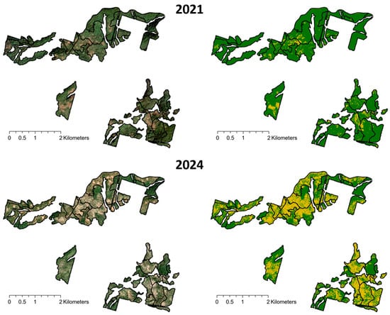
Figure 3.
Comparison of PlanetScope RGB imagery and U-Net CNN model predictions of forest canopy versus openings in the Alaska Peak project (2021 vs. 2024). Each row of panels corresponds to a single year of analysis, with 2021 (top) and 2024 (bottom), showing Alaska Peak treatment units at left in true-color Planet Basemap imagery (Bands 4–3–2) and their corresponding predicted canopy/opening masks at right. In the model-prediction panels, each pixel has been classified by a U-Net CNN (with residual blocks) trained on 2020 CFO canopy cover data and Planet Basemap 8-band surface reflectance imagery (see Section 2). Forest-covered pixels are shown in solid dark green, and canopy-opening pixels (predicted “non-forest,” <50% canopy cover) in yellow.
Further assessment of canopy patch size distributions (Figure 4; SI Figures S6–S7; detailed metrics in Table S2) indicated a marked increase in smaller forest patches (<0.25 acres), reflecting rapid proliferation and the breakup of previously continuous canopy cover. Conversely, areas covered by large (>5 acres) forest patches substantially declined as the project area shifted towards a finer-grained canopy mosaic. Correspondingly, the average size of canopy openings increased by more than fivefold, increasing from an average of 0.044 acres in 2020 to 0.418 acres in 2024.
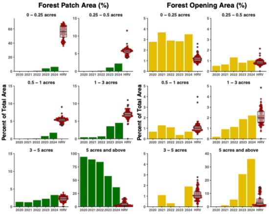
Figure 4.
Comparison of Alaska Peak canopy structure to HRV benchmarks, by size class (2020–2024). Each row of panels corresponds to one of six Historical Range of Variability (HRV) size-class bins: 0–0.25 acres, 0.25–0.5 acres, 0.5–1 acre, 1–3 acres, 3–5 acres, and ≥ 5 acres [56]. HRV values (red circles) represent the distribution of patch-area percentages across all subbasins in the Upper Yuba watershed [56], with overlaid boxplots depicting the median, interquartile range, and full range of HRV percentages. In the left column (green bars), the vertical axis shows the percentage of the total Alaska Peak treatment-unit area occupied by forest patches of the indicated size class in each year (2020–2024). In the right column (gold bars), the same size-class bins are used to display the percentage of total area comprising open-canopy polygons. For both forest patches and openings, polygons were generated by converting classified canopy-and-opening rasters (within treatment-unit boundaries) into vector features, assigning unique IDs, and computing area and perimeter in square meters (Section 2). Bars for 2020–2024 reflect annual totals.
The spatial analysis of distance-to-canopy edges (Figure 5; Table S3) provided additional insights into changing canopy spatial patterns. By 2024, approximately 56% of open canopy areas were situated within relatively short distances (6–12 m) from the nearest canopy edge, highlighting substantial edge proliferation. Simultaneously, more isolated openings, situated ≥24 m from the nearest canopy, expanded from negligible levels in 2020 to nearly 5% of the landscape by 2024.
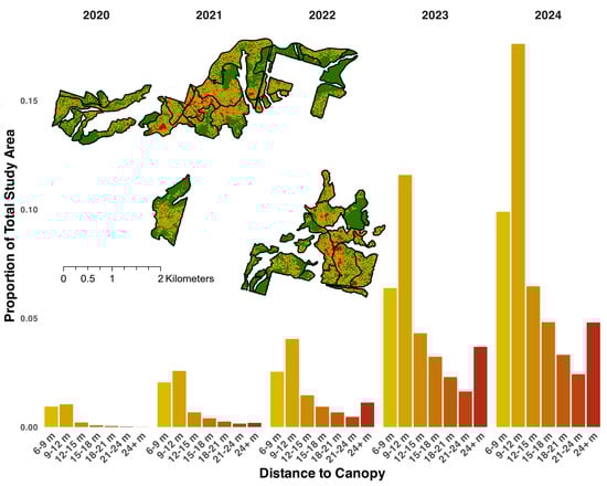
Figure 5.
Temporal distribution of open-canopy area by distance-to-canopy class (2020–2024). Bars show the proportion of the total study area occupied by open-canopy pixels in seven reclassified distance bins from the nearest forest canopy: 6–9 m, 9–12 m, 12–15 m, 15–18 m, 18–21 m, 21–24 m, and ≥24 m. Distances were calculated on a masked distance raster (following [13]) and binned in discrete intervals (see Methods). For each year, bar height represents the fraction of the study area within that distance class; bars are colored from pale yellow (6–9 m) through deep red (≥24 m) to emphasize increasing distance. Over the five-year period, total open-canopy area grows-most notably within the 6–12 m classes-indicating that new openings are predominantly occurring adjacent to existing canopy. Inset (upper left): Example map of opening-to-canopy distance classification in several Alaska Peak project units, with pixel colors corresponding yellow to red pixel colors corresponding to distance-to-canopy classes shown in histogram. Green pixels represent forest canopy, as predicted by CNN model.
4. Discussion
Land management agencies like the USDA Forest Service face the immense challenge of monitoring forest restoration outcomes across millions of acres with limited resources. The framework developed in this study directly addresses this operational bottleneck. By automating the analysis of high-resolution PlanetScope imagery using a CNN, our approach provides a scalable and resource-efficient method for tracking the fine-scale structural changes that define restoration treatment success. It further translates complex datasets into simple, actionable forest intelligence: annual (or sub-annual) maps of canopy openings and residual forest patches. This capability bridges the gap between expensive, infrequent LiDAR acquisitions and coarse-resolution satellite products, providing managers with timely data needed to inform adaptive management.
4.1. Model Performance and Validation Against Independent LiDAR Data
Independent validation against airborne LiDAR across 34,800 acres (140 km2) of diverse and varied terrain confirmed the model’s operational capability for land managers (SI Figures S1–S4). This performance occurred despite several challenges, including a spatial misalignment between 4.77 m PlanetScope pixels and LiDAR point clouds (e.g., [16]), a 2–3-month temporal offset between image and LiDAR acquisition, and fundamental definitional differences between training data (spectral-based < 50% canopy cover from CFO) and validation data (structural < 3 m height from LiDAR).
Analysis of prediction errors reveals that disagreements between model outputs and LiDAR reference data are concentrated overwhelmingly at forest-opening boundaries, occurring primarily in small, isolated patches of 1–3 pixels rather than large, systematic errors (SI Figures S1–S4). This pattern indicates the model successfully identifies the core areas of both gaps and canopy but shows uncertainty in the precise delineation of complex edges. Several factors may contribute to these edge disagreements: (1) the 50% canopy cover threshold used in training creates an inherently uncertain boundary zone where pixels near 50% coverage may be classified differently depending on slight variations in spectral signal; (2) the 3 m height threshold applied to LiDAR defines gaps differently than the spectral-based model, particularly in areas with tall shrubs or regeneration; and (3) areas of partial canopy cover, shadows, and understory vegetation create ambiguous spectral signatures. For management applications, such as assessing whether treatments successfully created openings of target sizes or reduced canopy continuity, this level of accuracy exceeds operational requirements.
4.2. Case Study: North Yuba Landscape Resilience Project
Applying this framework to the Alaska Peak Project revealed that fuel reduction treatments between 2020 and 2024 substantially altered the forest, shifting it from a dense, continuous canopy to a mosaic of patches and openings (Figure 3, Figure 4 and Figure 5; SI Figures S6–S7). The treatments successfully broke up large, continuous stands into numerous smaller patches, while creating nearly ten times more open area. However, a simple quantification of change does not fully capture the ecological outcomes. When compared to the HRV for the region, the 2024 post-treatment conditions show a departure from historical norms, with a higher-than-expected prevalence of large openings (>5 acres) and a deficit of small-to-medium forest patch classes. Thus, while treatments increased heterogeneity, the forest structure remains more homogenous than HRV conditions.
Even with the formation of these large openings, the distance-to-canopy analysis (Figure 5, sensu [6]) shows that a substantial proportion of the open area is within relatively short distances to canopy edges (e.g., 6–9 m, 9–12 m, 12–15 m), indicating that even the larger, connected openings often retain some degree of internal complexity. Rather than single, uniform open patches, many of these large openings include peninsulas of forest cover and irregular shapes that break up the continuity of non-forested areas.
Further, the observed surplus of openings larger than five acres is concentrated in the project’s even-aged pine plantations, which were established following the 1959 Mountain House fire [57]. These stands were at extreme risk of mortality, with stocking densities near 100% of their maximum capacity and containing pre-existing beetle-kill mortality pockets up to six acres in size. Consequently, prescriptions for these plantation units called for intensive rehabilitation, including the salvage of dead trees, the creation of large gaps to reset conditions for pine regeneration, and thinning to a low target density of 80 sq ft of basal area per acre to reduce crown-fire continuity. In contrast, prescriptions for the surrounding, naturally regenerated stands involved a lighter, variable density restoration treatment designed to leave an average of 160 sq ft of basal area per acre while creating a finer patchwork of smaller gaps and retained clumps. This contrast in prescriptions- intensive rehabilitation versus fine-grained restoration- explains why large new openings are largely confined to the plantations, while treatments in the naturally regenerated stands resulted in a structural complexity more aligned with HRV.
The treated units are also embedded within a complex matric of surrounding lands that are receiving different, less intensive management, including densely forested private inholdings, commercial timberlands on steep terrain, and California Spotted Owl and Northern Goshawk breeding habitat. Therefore, the creation of larger openings in these specific units should not be viewed in isolation, but as a deliberate contribution to a landscape-scale mosaic. These treatments introduce significant heterogeneity into an otherwise contiguous and high-risk forested area, thereby creating the varied structure that is ultimately more characteristic of a resilient, fire-adapted landscape than pre-treatment conditions.
From an ecological perspective, the results highlight both success and a need for more refined treatment but offer up the necessary monitoring feedback to close an adaptive management loop. The significant increase in structural complexity and edge habitat aligns with broad restoration objectives and can benefit wildlife that use these ecotones between forest and open areas. For example, California Spotted Owls have been observed to hunt along the edges of newly formed openings post-wildfire [30] and varied opening sizes can benefit multiple species [58,59]. However, the higher prevalence of large openings (>5 ac) can lead to unintended outcomes for tree seedling survival and regeneration due to limited seed availability, increased competition from shrubs, and harsher moisture and temperature regimes [60,61]. Adjusting thinning prescriptions or group selection approaches, for example, by distributing openings more evenly across historically common sizes (0.1–3 ac), limiting contiguous openings, aligning openings with areas characterized by low tree densities (e.g., south facing slopes) or retaining canopy clumps, could help preserve the ecological functions of smaller, interspersed openings while still meeting fuel reduction goals [4].
Beyond this project-level analysis, the CNN-based framework offers a valuable way to monitor forest structure across the broader TCSI region. While programs like Monitoring Trends in Burn Severity (MTBS) provide important large-scale burn severity data [55], their coarser resolution can miss fine-scale heterogeneity, such as small refugia or subtle mortality patterns and do not track changes following mechanical treatments [62]. This PlanetScope-based approach enables the identification of smaller patches and openings, improving our ability to identify and track fire refugia, habitat edges, and residual canopy structures that are important for wildlife [63,64].
4.3. Limitations
Several limitations of this study present opportunities to improve its application to monitoring. First, the model was trained using single-season (summer) imagery; its performance on data from other seasons, which may contain different sun angles or phenological states, is unknown. Future work could explore the use of multi-temporal inputs to improve model robustness to time of year. Second, the binary classification of ‘opening’ does not differentiate between bare ground, shrub cover, herbaceous understory, or varying degrees of canopy cover, all of which of distinct implications for fire dynamics. Integrating additional data sources, such as spectral unmixing or LiDAR, could help resolve this ambiguity. Third, comparisons to HRV benchmarks are approximate because our CNN detects openings spectrally at 4.77 m resolution, while HRV define openings using tree height thresholds and neighborhood-based canopy cover at coarser scales. Finally, while the framework is designed to be adaptable, the current model has only been validated in Sierra Nevada mixed-conifer forests and would require retraining for application in other forest types.
5. Conclusions
This study demonstrates how high spatiotemporal resolution multispectral imagery and CNNs can reveal fine-scale transformations in forest canopy structure driven by active management. At Alaska Peak, our approach highlights opportunities to monitor treatment effectiveness and adapt prescriptions to maintain ecological complexity. Across broader landscapes, agencies can apply this framework to more accurately track forest change, pinpoint management priorities, and refine strategies to help improve resilience in fire-adapted forests.
The workflow developed here has direct applicability beyond the North Yuba CFLRP. CFLRP projects across the western United States face similar monitoring challenges of tracking fine-scale structural outcomes across large, remote landscapes with limited resources. Because the approach relies on commercially available PlanetScope imagery and widely used deep learning frameworks, it can be adapted to other fire-prone forest systems where canopy structure is a key management objective, though retraining would be required for forest types with different structural characteristics.
This framework also offers potential for integration with existing forest monitoring programs. Federal agencies currently rely on field plots, Landsat-based products like the Landscape Change Monitoring System (LCMS), and periodic LiDAR acquisitions to assess forest conditions. Our approach addresses a scale gap in this toolkit, capturing fine-scale structural changes that Landsat-based products cannot resolve while offering greater temporal frequency and lower cost than LiDAR. This complements existing monitoring programs by providing detailed canopy structure information within landscapes or fire perimeters identified through coarser-resolution change detection. By translating satellite imagery into validated, actionable metrics of forest structure, this workflow provides a scalable foundation for monitoring restoration outcomes across fire-prone western forests.
Supplementary Materials
The following supporting information can be downloaded at: https://www.mdpi.com/article/10.3390/rs18020346/s1, Figure S1: Spatial Distribution of False Positive Errors. Histogram showing the total number of false positive (FP) pixels (pixels incorrectly classified as ‘gap’) as a function of their distance to the nearest true gap edge, aggregated across all 125 validation tiles. The distribution is strongly skewed toward zero, indicating that the vast majority of false positive errors occur immediately adjacent to or within a few meters of a true canopy gap boundary. Figure S2: Spatial Distribution of False Negative Errors. Histogram showing the total number of false negative (FN) pixels (pixels where a true ‘gap’ was missed) as a function of their distance to the nearest true forest edge, aggregated across all validation tiles. The analysis shows that errors of omission are almost exclusively located directly at the forest-gap interface, with a sharp drop-off in frequency beyond the first few meters. Figure S3: Size Distribution of False Positive Error Patches. Density histogram of contiguous false positive (FP) patch sizes, measured in number of pixels (~4.77 m resolution). The distribution shows that most erroneous FP predictions occur in very small, isolated patches, with the highest density corresponding to single-pixel errors. This pattern suggests that errors are localized and do not form large, contiguous areas of misclassification. The y-axis represents frequency of patches that fall within each patch size (number of pixels). Figure S4: Size Distribution of False Negative Error Patches. Density histogram of contiguous false negative (FN) patch sizes, measured in number of pixels. Similar to false positives, the majority of false negative errors occur in small clumps of just a few pixels. This reinforces that model disagreements with the LiDAR reference are concentrated in fine-scale, localized areas, typically along complex canopy edges, rather than large, systemic errors. The y-axis represents frequency of patches that fall within each patch size (number of pixels). Figure S5. Annual spatial predictions of forest canopy and open-canopy cover in the Alaska Peak restoration and fuels-reduction project, 2020–2024. Each year’s map shows the Alaska Peak treatment-unit polygons overlaid on predicted canopy-cover masks generated by our U-Net CNN. Within each unit, green pixels denote model-predicted “forest” (≥50% canopy cover), and yellow pixels denote “opening” (<50% canopy cover). Predictions were produced by applying the trained U-Net (with residual blocks) to Planet Basemap multispectral imagery (≈4.77 m resolution) for the third quarter (July–September) in 2020–2023 and September imagery only in 2024. For each input tile (64 × 64 pixels), the model ingested 15 channels (8 Planet Basemap bands, 4 spectral indices [NDVI, NDRE, GNDVI, VARI], and 3 DEM-derived layers [elevation, slope, aspect]) and output a per-pixel open-canopy probability map (threshold at 0.5). By visualizing the annual masks side by side, this figure illustrates how canopy openings emerged and expanded across treatment units following fuels-reduction activities and natural disturbances over the five-year period. Figure S6. Annual area in acres of forest patches (left) and canopy openings (right) by HRV size-class bins in the Alaska Peak treatment units, 2020 to 2024. Each panel corresponds to one of six Historical Range of Variability size classes (0 to 0.25 acres, 0.25 to 0.5 acres, 0.5 to 1 acre, 1 to 3 acres, 3 to 5 acres, and 5 acres or more) and shows the total area of all polygons derived from the U-Net CNN canopy and opening predictions within that class for each year. Forest patches are shown as green bars on the left side of each pair, and canopy openings are shown as yellow bars on the right. From 2020 to 2024, large forest patches (5 acres or more) declined steadily from 1170.7 acres to 456.7 acres, while smaller patches (under 3 acres) increased as treatments fragmented the canopy. In contrast, canopy openings of 5 acres or more appeared after 2021 and reached 448.2 acres in 2024, and openings in the 1 to 3-acre class grew from 2.5 acres to 27.6 acres, indicating that fuels-reduction activities and natural disturbances produced more and larger canopy gaps over time. Figure S7. Annual counts of forest patches (left) and canopy openings (right) by size-class bins in the Alaska Peak treatment units, 2020 to 2024. Each panel corresponds to one of six Historical Range of Variability size classes (0 to 0.25 acres, 0.25 to 0.5 acres, 0.5 to 1 acre, 1 to 3 acres, 3 to 5 acres, and 5 acres or more) and shows the total number of individual polygons derived from U-Net CNN predictions within that class each year. Forest patch counts are shown as green bars, and opening counts are shown as yellow bars. Between 2020 and 2024, the number of very small forest patches (0 to 0.25 acres) increased from 74 to 2169, while patches in the 1 to 3-acre and 5-acre-or-more classes also rose steadily. In contrast, the count of very small openings (0 to 0.25 acres) remained above 1100 each year, and openings in the 1 to 3-acre class grew from 2 to 18, indicating that treatments and disturbances created more small canopy gaps over time. Table S1. Performance of the best-performing U-Net CNN on the independent test set of California Forest Observatory (Salo Sciences, 2020) canopy cover data (batch size 64). The table reports accuracy, precision, recall, F1-score, Dice coefficient, and ROC-AUC. Table S2. Annual statistics of forest patch area and canopy opening area by size class within the Alaska Peak treatment units from 2020 to 2024. For each habitat type (forest or opening), year, and size class (0 to 0.25 acres, 0.25 to 0.5 acres, 0.5 to 1 acre, 1 to 3 acres, 3 to 5 acres, and 5 acres or more), the table lists the total area (in acres), mean patch area, median patch area, standard deviation of patch area (all in acres), and the total number of patches. Table S3. Annual area in acres and proportion of the study area occupied by forest openings in each distance-to-canopy class, 2020 to 2024. For each year and each 3-meter distance bin (6 to 9 m, 9 to 12 m, 12 to 15 m, 15 to 18 m, 18 to 21 m, 21 to 24 m, and 24 m or more from the nearest canopy), the table shows the total opening area in acres and the fraction of the total study area covered by those openings. Distances were calculated on a masked distance raster measuring the distance from each opening pixel to the nearest canopy clump. Text S1: Extended study-area and treatment context. Text S2: Extended data preparation & acquisition details. Text S3: Detailed CNN architecture & hyper-parameters. Text S4: Alaska Peak GIS & HRV-bin processing details. Text S5: Extended Results.
Author Contributions
J.N.H. conceived the study, developed the methodology, performed all analyses, and wrote the original manuscript. B.L.E. provided key input on the manuscript’s focus and interpretation, and consulted on the Historic Range of Variability (HRV) analyses and method applicability. K.N.W. contributed to manuscript writing and application of method. All authors have read and agreed to the published version of the manuscript.
Funding
This project was supported by the North Yuba Forest Partnership (CFLR029) under the Collaborative Forest Land-scape Restoration Program (CFLRP).
Data Availability Statement
Upon publication of this manuscript, the data products and code generated during this study will be deposited in a permanent public repository. This includes: (1) the trained residual U-Net model and the Python scripts used for model training and analysis; (2) the final geospatial outputs, including annual (2020–2024) raster and vector maps of canopy cover and openings within the Alaska Peak Project area; and (3) all derived tabular data, such as the patch size and distance-to-canopy metrics. The geospatial boundary files for the study region will also be provided. The proprietary PlanetScope imagery used for the analysis cannot be shared due to licensing restrictions. The California Forest Observatory (CFO) data used to create reference masks for model training is publicly available.
Acknowledgments
We extend our gratitude to Michèle Slaton for her invaluable feedback on the analytical approach and the manuscript, which greatly improved the quality of this work. We are also grateful to Francesco Tonini for his assistance in acquiring the geospatial imagery through Planet, and to Kyle Taylor for providing background on the Alaska Peak Project area and silvicultural approaches.
Conflicts of Interest
The authors declare no conflicts of interest.
References
- Larson, A.J.; Churchill, D. Tree Spatial Patterns in Fire-Frequent Forests of Western North America, Including Mechanisms of Pattern Formation and Implications for Designing Fuel Reduction and Restoration Treatments. For. Ecol. Manag. 2012, 267, 74–92. [Google Scholar] [CrossRef]
- Stephens, S.L.; Collins, B.M.; Biber, E.; Fulé, P.Z. U.S. Federal Fire and Forest Policy: Emphasizing Resilience in Dry Forests. Ecosphere 2016, 7, e01584. [Google Scholar] [CrossRef]
- Churchill, D.J.; Larson, A.J.; Dahlgreen, M.C.; Franklin, J.F.; Hessburg, P.F.; Lutz, J.A. Restoring Forest Resilience: From Reference Spatial Patterns to Silvicultural Prescriptions and Monitoring. For. Ecol. Manag. 2013, 291, 442–457. [Google Scholar] [CrossRef]
- Hessburg, P.F.; Churchill, D.J.; Larson, A.J.; Haugo, R.D.; Miller, C.; Spies, T.A.; North, M.P.; Povak, N.A.; Belote, R.T.; Singleton, P.H.; et al. Restoring Fire-Prone Inland Pacific Landscapes: Seven Core Principles. Landsc. Ecol. 2015, 30, 1805–1835. [Google Scholar] [CrossRef]
- Lydersen, J.M.; North, M.P.; Knapp, E.E.; Collins, B.M. Quantifying Spatial Patterns of Tree Groups and Gaps in Mixed-Conifer Forests: Reference Conditions and Long-Term Changes Following Fire Suppression and Logging. For. Ecol. Manag. 2013, 304, 370–382. [Google Scholar] [CrossRef]
- Jeronimo, S.M.A.; Kane, V.R.; Churchill, D.J.; Lutz, J.A.; North, M.P.; Asner, G.P.; Franklin, J.F. Forest Structure and Pattern Vary by Climate and Landform across Active-Fire Landscapes in the Montane Sierra Nevada. For. Ecol. Manag. 2019, 437, 70–86. [Google Scholar] [CrossRef]
- Fertel, H.M.; North, M.P.; Latimer, A.M.; Ng, J. Growth and Spatial Patterns of Natural Regeneration in Sierra Nevada Mixed-Conifer Forests with a Restored Fire Regime. For. Ecol Manag. 2022, 519, 120270. [Google Scholar] [CrossRef]
- Camarretta, N.; Harrison, P.A.; Bailey, T.; Potts, B.; Lucieer, A.; Davidson, N.; Hunt, M. Monitoring Forest Structure to Guide Adaptive Management of Forest Restoration: A Review of Remote Sensing Approaches. New For. 2020, 51, 573–596. [Google Scholar] [CrossRef]
- Massey, R.; Berner, L.T.; Foster, A.C.; Goetz, S.J.; Vepakomma, U. Remote Sensing Tools for Monitoring Forests and Tracking Their Dynamics. In Boreal Forests in the Face of Climate Change; Springer: Cham, Switzerland, 2023; pp. 637–655. [Google Scholar]
- Pause, M.; Schweitzer, C.; Rosenthal, M.; Keuck, V.; Bumberger, J.; Dietrich, P.; Heurich, M.; Jung, A.; Lausch, A. In Situ/Remote Sensing Integration to Assess Forest Health—A Review. Remote Sens. 2016, 8, 471. [Google Scholar] [CrossRef]
- Fassnacht, F.E.; White, J.C.; Wulder, M.A.; Næsset, E. Remote Sensing in Forestry: Current Challenges, Considerations and Directions. Forestry 2024, 97, 11–37. [Google Scholar] [CrossRef]
- Kane, V.R.; Bartl-Geller, B.N.; North, M.P.; Kane, J.T.; Lydersen, J.M.; Jeronimo, S.M.A.; Collins, B.M.; Monika Moskal, L. First-Entry Wildfires Can Create Opening and Tree Clump Patterns Characteristic of Resilient Forests. For. Ecol. Manag. 2019, 454, 117659. [Google Scholar] [CrossRef]
- Olszewski, J.; Bienz, C.; Markus, A. Using Airborne LiDAR to Monitor Spatial Patterns in South Central Oregon Dry Mixed-Conifer Forest. J. For. 2022, 120, 714–727. [Google Scholar] [CrossRef]
- Churchill, D.J.; Carnwath, G.C.; Larson, A.J.; Jeronimo, S.A. Historical Forest Structure, Composition, and Spatial Pattern in Dry Conifer Forests of the Western Blue Mountains, Oregon; USDA: Portland, OR, USA, 2017.
- Liu, S.; Brandt, M.; Nord-Larsen, T.; Chave, J.; Reiner, F.; Lang, N.; Tong, X.; Ciais, P.; Igel, C.; Pascual, A.; et al. The Overlooked Contribution of Trees Outside Forests to Tree Cover and Woody Biomass across Europe. Sci. Adv. 2023, 9, eadh4097. [Google Scholar] [CrossRef]
- Dixon, D.J.; Zhu, Y.; Jin, Y. Canopy Height Estimation from PlanetScope Time Series with Spatio-Temporal Deep Learning. Remote Sens. Environ. 2024, 318, 114518. [Google Scholar] [CrossRef]
- Francini, S.; McRoberts, R.E.; Giannetti, F.; Mencucci, M.; Marchetti, M.; Scarascia Mugnozza, G.; Chirici, G. Near-Real Time Forest Change Detection Using PlanetScope Imagery. Eur. J. Remote Sens. 2020, 53, 233–244. [Google Scholar] [CrossRef]
- Reiner, F.; Gominski, D.; Fensholt, R.; Brandt, M. An Operational Framework to Track Individual Farmland Trees over Time at National Scales Using PlanetScope. IEEE J. Sel. Top. Appl. Earth Obs. Remote Sens. 2025, 18, 1109–1121. [Google Scholar] [CrossRef]
- Wagner, F.H.; Dalagnol, R.; Silva-Junior, C.H.L.; Carter, G.; Ritz, A.L.; Hirye, M.C.M.; Ometto, J.P.H.B.; Saatchi, S. Mapping Tropical Forest Cover and Deforestation with Planet NICFI Satellite Images and Deep Learning in Mato Grosso State (Brazil) from 2015 to 2021. Remote Sens. 2023, 15, 521. [Google Scholar] [CrossRef]
- Hobi, M.L.; Ginzler, C.; Commarmot, B.; Bugmann, H. Gap Pattern of the Largest Primeval Beech Forest of Europe Revealed by Remote Sensing. Ecosphere 2015, 6, 1–15. [Google Scholar] [CrossRef]
- Maxwell, C.J.; Scheller, R.M.; Wilson, K.N.; Manley, P.N. Assessing the Effectiveness of Landscape-Scale Forest Adaptation Actions to Improve Resilience under Projected Climate Change. Front. For. Glob. Change 2022, 5, 740869. [Google Scholar] [CrossRef]
- Avery, A.; Vasques, J.; Ilano, E.; Walker, E.; Stout, J.; Barhydt, R.; Porter, D.; Brink, S.; Millar, M. TAHOE-CENTRAL SIERRA INITIATIVE 10-YEAR REGIONAL PLAN Advancing State and Federal Commitments to Restore Resilience. 2023. Available online: https://www.tahoecentralsierra.org/wp-content/uploads/2023/09/1.-TCSI-10-Year-Regional-Plan.pdf (accessed on 1 January 2025).
- U.S. Forest Service. North Yuba Landscape Resilience Project; Final Environmental Impact Statement; U.S. Forest Service: Nevada city, CA, USA, 2023.
- Planet Labs BBC. PlanetScope Product Specifications; Planet Labs BBC: San Francisco, CA, USA, 2023. [Google Scholar]
- Salo Sciences. California Forest Observatory Data Description: Vegetation Structure & Fuels; Salo Sciences, Inc.: San Francisco, CA, USA, 2020. [Google Scholar]
- Wilkinson, Z.A.; Kramer, H.A.; Jones, G.M.; Zulla, C.J.; McGinn, K.; Barry, J.M.; Sawyer, S.C.; Tanner, R.; Gutiérrez, R.J.; Keane, J.J.; et al. Tall, Heterogeneous Forests Improve Prey Capture, Delivery to Nestlings, and Reproductive Success for Spotted Owls in Southern California. Ornithol. Appl. 2023, 125, duac048. [Google Scholar] [CrossRef]
- Chamberlain, C.P.; Cova, G.R.; Kane, V.R.; Cansler, C.A.; Kane, J.T.; Bartl-Geller, B.N.; van Wagtendonk, L.; Jeronimo, S.M.A.; Stine, P.; North, M.P. Sierra Nevada Reference Conditions: A Dataset of Contemporary Reference Sites and Corresponding Remote Sensing-Derived Forest Structure Metrics for Yellow Pine and Mixed-Conifer Forests. Data Brief 2023, 51, 109807. [Google Scholar] [CrossRef] [PubMed]
- Kramer, H.A.; Kelly, K.G.; Whitmore, S.A.; Berigan, W.J.; Reid, D.S.; Wood, C.M.; Klinck, H.; Kahl, S.; Manley, P.N.; Sawyer, S.C.; et al. Using Bioacoustics to Enhance the Efficiency of Spotted Owl Surveys and Facilitate Forest Restoration. J. Wildl. Manag. 2024, 88, e22533. [Google Scholar] [CrossRef]
- Zulla, C.J.; Jones, G.M.; Kramer, H.A.; Keane, J.J.; Roberts, K.N.; Dotters, B.P.; Sawyer, S.C.; Whitmore, S.A.; Berigan, W.J.; Kelly, K.G.; et al. Forest Heterogeneity Outweighs Movement Costs by Enhancing Hunting Success and Reproductive Output in California Spotted Owls. Landsc. Ecol. 2023, 38, 2655–2673. [Google Scholar] [CrossRef]
- Wright, M.E.; Zachariah Peery, M.; Ayars, J.; Dotters, B.P.; Roberts, K.N.; Jones, G.M. Fuels Reduction Can Directly Improve Spotted Owl Foraging Habitat in the Sierra Nevada. For. Ecol Manag. 2023, 549, 121430. [Google Scholar] [CrossRef]
- Hansen, M.C.; Potapov, P.V.; Moore, R.; Hancher, M.; Turubanova, S.A.; Tyukavina, A.; Thau, D.; Stehman, S.V.; Goetz, S.J.; Loveland, T.R.; et al. High-Resolution Global Maps of 21st-Century Forest Cover Change. Science 2013, 342, 850–853. [Google Scholar] [CrossRef]
- Huete, A.; Didan, K.; Miura, T.; Rodriguez, E.P.; Gao, X.; Ferreira, L.G. Overview of the Radiometric and Biophysical Performance of the MODIS Vegetation Indices. Remote Sens. Environ. 2002, 83, 195–213. [Google Scholar] [CrossRef]
- Gitelson, A.A.; Kaufman, Y.J.; Merzlyak, M.N. Use of a Green Channel in Remote Sensing of Global Vegetation from EOS-MODIS. Remote Sens. Environ. 1996, 58, 289–298. [Google Scholar] [CrossRef]
- Franklin, J. Predictive Vegetation Mapping: Geographic Modelling of Biospatial Patterns in Relation to Environmental Gradients. Prog. Phys. Geogr. Earth Environ. 1995, 19, 474–499. [Google Scholar] [CrossRef]
- Farr, T.G.; Rosen, P.A.; Caro, E.; Crippen, R.; Duren, R.; Hensley, S.; Kobrick, M.; Paller, M.; Rodriguez, E.; Roth, L.; et al. The Shuttle Radar Topography Mission. Rev. Geophys. 2007, 45, RG2004. [Google Scholar] [CrossRef]
- Zeiler, M.D.; Fergus, R. Visualizing and Understanding Convolutional Networks. In Computer Vision—ECCV 2014. Proceeding of 13th European Conference, Zurich, Switzerland, 12 September 2014; Springer: Cham, Switzerland, 2014; pp. 818–833. [Google Scholar]
- Simonyan, K.; Zisserman, A. Very Deep Convolutional Networks for Large-Scale Image Recognition. arXiv 2014, arXiv:1409.1556. [Google Scholar]
- Ronneberger, O.; Fischer, P.; Brox, T. U-Net: Convolutional Networks for Biomedical Image Segmentation. In Medical Image Computing and Computer-Assisted Intervention—MICCAI 2015. Proceeding of 18th International Conference, Munich, Germany, 5–9 October 2015; Springer: Cham: Switzerland, 2015; pp. 234–241. [Google Scholar]
- He, K.; Zhang, X.; Ren, S.; Sun, J. Deep Residual Learning for Image Recognition. In Proceedings of the 2016 IEEE Conference on Computer Vision and Pattern Recognition (CVPR), Las Vegas, NV, USA, 27–30 June 2016; IEEE: New York, NY, USA, 2015. [Google Scholar]
- Drozdzal, M.; Vorontsov, E.; Chartrand, G.; Kadoury, S.; Pal, C. The Importance of Skip Connections in Biomedical Image Segmentation. In Deep Learning and Data Labeling for Medical Applications. Proceeding of First International Workshop, LABELS 2016, and Second International Workshop, DLMIA 2016, Held in Conjunction with MICCAI 2016, Athens, Greece, 21 October 2016; Springer: Cham, Switzerland, 2016. [Google Scholar]
- Siddique, N.; Paheding, S.; Elkin, C.P.; Devabhaktuni, V. U-Net and Its Variants for Medical Image Segmentation: A Review of Theory and Applications. IEEE Access 2021, 9, 82031–82057. [Google Scholar] [CrossRef]
- Kingma, D.P.; Ba, J. Adam: A Method for Stochastic Optimization. arXiv 2014, arXiv:1412.6980. [Google Scholar]
- Goodfellow, I.; Bengio, Y.; Courville, A. Deep Learning; The MIT Press: Cambridge, MA, USA, 2016; ISBN 0262035618. [Google Scholar]
- de Boer, P.-T.; Kroese, D.P.; Mannor, S.; Rubinstein, R.Y. A Tutorial on the Cross-Entropy Method. Ann. Oper. Res. 2005, 134, 19–67. [Google Scholar] [CrossRef]
- Abadi, M.; Barham, P.; Chen, J.; Chen, Z.; Davis, A.; Dean, J.; Devin, M.; Ghemawat, S.; Irving, G.; Isard, M.; et al. TensorFlow: A System for Large-Scale Machine Learning. arXiv 2016, arXiv:1605.08695. [Google Scholar]
- Chollet, F. Keras. 2015. Available online: https://keras.io (accessed on 1 January 2025).
- USGS. 3D Elevation Program (3DEP) Lidar Point Cloud: CA Sierra Nevada B22 [Dataset]; USGS: Reston, VA, USA, 2022. [Google Scholar]
- Roussel, J.R.; Auty, D.; Coops, N.C.; Tompalski, P.; Goodbody, T.R.H.; Meador, A.S.; Bourdon, J.F.; de Boissieu, F.; Achim, A. LidR: An R Package for Analysis of Airborne Laser Scanning (ALS) Data. Remote Sens. Environ. 2020, 251, 112061. [Google Scholar] [CrossRef]
- Zhang, W.; Qi, J.; Wan, P.; Wang, H.; Xie, D.; Wang, X.; Yan, G. An Easy-to-Use Airborne LiDAR Data Filtering Method Based on Cloth Simulation. Remote Sens. 2016, 8, 501. [Google Scholar] [CrossRef]
- Pfeifer, N.; Reiter, T.; Briese, C.; Rieger, W. Interpolation of High Quality Ground Models from Laser Scanner Data in Forested Areas. In International Archives of Photogrammetry and Remote Sensing. Proceeding of ISPRS Workshop, La Jolla, CA, USA, 9–11 November 1999; ISPRS: Beijing, China, 1999. [Google Scholar]
- Bonnet, S.; Gaulton, R.; Lehaire, F.; Lejeune, P. Canopy Gap Mapping from Airborne Laser Scanning: An Assessment of the Positional and Geometrical Accuracy. Remote Sens. 2015, 7, 11267–11294. [Google Scholar] [CrossRef]
- Goodbody, T.R.H.; Tompalski, P.; Coops, N.C.; White, J.C.; Wulder, M.A.; Sanelli, M. Uncovering Spatial and Ecological Variability in Gap Size Frequency Distributions in the Canadian Boreal Forest. Sci. Rep. 2020, 10, 6069. [Google Scholar] [CrossRef]
- Jia, K.; Liang, S.; Zhang, N.; Wei, X.; Gu, X.; Zhao, X.; Yao, Y.; Xie, X. Land Cover Classification of Finer Resolution Remote Sensing Data Integrating Temporal Features from Time Series Coarser Resolution Data. ISPRS J. Photogramm. Remote Sens. 2014, 93, 49–55. [Google Scholar] [CrossRef]
- Radoux, J.; Lamarche, C.; Van Bogaert, E.; Bontemps, S.; Brockmann, C.; Defourny, P. Automated Training Sample Extraction for Global Land Cover Mapping. Remote Sens 2014, 6, 3965–3987. [Google Scholar] [CrossRef]
- Finco, M.; Quayle, B.; Zhang, Y.; Lecker, J.; Megown, K.A.; Kenneth Brewer, C. Moving from Status to Monitoring Trends And Burn Severity (MTBS): Monitoring Wildfire Activity for the Past Quarter Century Using Landsat Data; USDA: Washington, DC, USA, 2012.
- McGarigal, K.; (Department of Environmental Conservation, University of Massachusetts Amherst, Amherst, MA, USA); Estes, B.L.; (U.S. Forest Service, Fort Collins, CO, USA); Conway, S.; Perrot, D.; Tierney, M.; (U.S. Forest Service, Fort Collins, CO, USA); Walsh, T.; (U.S. Forest Service, Fort Collins, CO, USA); Liang, C.; Smith, E. Northern Sierra Historical Range of Variability and Current Landscape Departure. Unpublished work. 2022. [Google Scholar]
- Brown, R. Trapper Project Silviculture Analysis; USDA Forest Service; Tahoe National Forest: Nevada City, CA, USA, 2020. Available online: https://usfs-public.app.box.com/v/PinyonPublic/file/934109640532 (accessed on 1 January 2025).
- White, A.M.; Zipkin, E.F.; Manley, P.N.; Schlesinger, M.D. Conservation of Avian Diversity in the Sierra Nevada: Moving beyond a Single-Species Management Focus. PLoS ONE 2013, 8, e63088. [Google Scholar] [CrossRef]
- Stephens, S.L.; Bigelow, S.W.; Burnett, R.D.; Collins, B.M.; Gallagher, C.V.; Keane, J.; Kelt, D.A.; North, M.P.; Roberts, L.J.; Stine, P.A.; et al. California Spotted Owl, Songbird, and Small Mammal Responses to Landscape Fuel Treatments. Bioscience 2014, 64, 893–906. [Google Scholar] [CrossRef]
- Gray, A.N.; Spies, T. Microsite Controls on Tree Seedling Establishment In Conifer Forest Canopy Gaps. Ecology 1997, 78, 2458–2473. [Google Scholar] [CrossRef]
- York, R.A.; Battles, J.J.; Heald, R.C. Edge Effects in Mixed Conifer Group Selection Openings: Tree Height Response to Resource Gradients. For. Ecol. Manag. 2003, 179, 107–121. [Google Scholar] [CrossRef]
- Howe, A.A.; Parks, S.A.; Harvey, B.J.; Saberi, S.J.; Lutz, J.A.; Yocom, L.L. Comparing Sentinel-2 and Landsat 8 for Burn Severity Mapping in Western North America. Remote Sens. 2022, 14, 5249. [Google Scholar] [CrossRef]
- Kolden, C.A.; Abatzoglou, J.T.; Lutz, J.A.; Cansler, C.A.; Kane, J.T.; Van Wagtendonk, J.W.; Key, C.H. Climate Contributors to Forest Mosaics: Ecological Persistence Following Wildfire. Proc. Northwest Sci. 2015, 89, 219–238. [Google Scholar] [CrossRef]
- Meddens, A.J.H.; Kolden, C.A.; Lutz, J.A.; Smith, A.M.S.; Cansler, C.A.; Abatzoglou, J.T.; Meigs, G.W.; Downing, W.M.; Krawchuk, M.A. Fire Refugia: What Are They, and Why Do They Matter for Global Change? Bioscience 2018, 68, 944–954. [Google Scholar] [CrossRef]


Disclaimer/Publisher’s Note: The statements, opinions and data contained in all publications are solely those of the individual author(s) and contributor(s) and not of MDPI and/or the editor(s). MDPI and/or the editor(s) disclaim responsibility for any injury to people or property resulting from any ideas, methods, instructions or products referred to in the content. |
© 2026 by the authors. Licensee MDPI, Basel, Switzerland. This article is an open access article distributed under the terms and conditions of the Creative Commons Attribution (CC BY) license.