Lightweight Complex-Valued Siamese Network for Few-Shot PolSAR Image Classification

Highlights

What are the main findings?

• A novel lightweight complex-valued Siamese network is proposed for robust PolSAR image classification with very limited labeled data.
• The architecture effectively captures discriminative scattering and spatial features, achieving high classification accuracy while significantly reducing computational complexity (FLOPs) and parameters.

What is the implication of the main finding?

• The method provides a practical and data-efficient solution, overcoming the critical challenge of label scarcity in PolSAR image classification.
• The framework demonstrates strong potential for deploying high-precision PolSAR classification systems on hardware-limited devices.

Abstract

Complex-valued convolutional neural networks (CVCNNs) have demonstrated strong capabilities for polarimetric synthetic aperture radar (PolSAR) image classification by effectively integrating both amplitude and phase information inherent in polarimetric data. However, their practical deployment faces significant challenges due to high computational costs and performance degradation caused by extremely limited labeled samples. To address these challenges, a lightweight CV Siamese network (LCVSNet) is proposed for few-shot PolSAR image classification. Considering the constraints of limited hardware resources in practical applications, simple one-dimensional (1D) CV convolutions along the scattering dimension are combined with two-dimensional (2D) lightweight CV convolutions. In this way, the inter-element dependencies of polarimetric coherency matrix and the spatial correlations between neighboring units can be captured effectively, while simultaneously reducing computational costs. Furthermore, LCVSNet incorporates a contrastive learning (CL) projection head to explicitly optimize the feature space. This optimization can effectively enhance the feature discriminability, leading to accurate classification with a limited number of labeled samples. Experiments on three real PolSAR datasets demonstrate the effectiveness and practical utility of LCVSNet for PolSAR image classification with a small number of labeled samples.

1. Introduction

Polarimetric synthetic aperture radar (PolSAR) can provide continuous monitoring regardless of weather and lighting conditions. Compared to SAR, PolSAR can alter the polarization pattern of the electromagnetic waves during both reception and transmission, thereby obtaining richer target scattering information [1,2]. In this way, PolSAR technology has found widespread application across various domains [3,4,5,6,7,8,9].

Recently, driven by advances in computer hardware, deep learning has shown excellent performance in various applications [10,11] and has gradually become the dominant approach for classifying PolSAR images. Zhou et al. [12] are the first to apply convolutional neural network (CNN) to PolSAR image classification. Dong et al. proposed lightweight 3D convolutional networks to reduce the computational burden of 3D-CNN while maintaining competitive accuracy for PolSAR classification [13]. Wang et al. [14] leveraged wavelet-based transform convolution to extract local frequency features. Song et al. [15] employed a complex-valued graph U-Net coupled with a hierarchical-aware structure to extract multi-scale complex features, which are adaptively fused through a multi-scale attention mechanism. Although these networks leverage various techniques to extract deep polarimetric features and achieve high classification accuracy, they generally rely on fully supervised training with a substantial number of labeled samples, which is labor-intensive and time-consuming. With insufficient labeled samples, the networks are prone to overfitting, leading to degraded recognition performance. To address this problem of sample scarcity, semi-supervised and self-supervised learning (SSL) are two prominent approaches, which aim to enhance classification ability by exploiting unlabeled data.

Semi-supervised learning extends the training set by utilizing prior information from unlabeled samples. It then designs an additional loss term for the unlabeled data, which is incorporated into the objective function. Consequently, in addition to labeled samples, unlabeled samples can also provide valuable information for network training [16]. Bi et al. utilized the Markov random field (MRF) to promote the smoothness of class labels, facilitating label propagation. Then, the CNN is optimized using the augmented labeled data and iteratively predicts new labels for further label propagation [17]. In [18], the k-means algorithm is used to assign pseudo-labels to unlabeled samples, which are then included in the training set. Finally, a 3DCNN is trained using a weighted loss incorporating labeled samples, pseudo-labeled samples, and fusion data. In our previous work [19], we propose a semi-supervised CV network that creates and iteratively refines pseudo-labels for unlabeled samples during the training process. In the objective function, the losses from the pseudo-label samples serve as a regularization term to enhance model generalization. However, since unreliable sample-label pairs may cause the accumulation and propagation of errors, the introduction of unlabeled samples does not guarantee an improvement in network performance [20].

SSL leverages intrinsic data relationships to construct pretext tasks, generating supervisory signals from unlabeled data and facilitating the learning of transferable representations for downstream tasks [21,22]. As a dominant SSL paradigm, contrastive learning (CL) has shown remarkable efficacy in few-shot classification by addressing the critical challenge of label scarcity. For instance, Zhang et al. proposed a CL framework that designs instance discrimination as a pretext task to extract useful representations from unlabeled data [23]. Zhang et al. designed a novel encoder based on dynamic convolution and channel attention, which enhances CL while eliminating the need for negative samples [24]. Qiu et al. improved CL through a multi-scale feature fusion model and a mix-up auxiliary pathway, extracting more comprehensive features from unlabeled data [25]. Furthermore, Dong et al. integrated CL with a vision transformer-based architecture to capture long-range dependencies, thus learning robust representations [26]. These classification results demonstrate the advantages and potential of CL-based models for few-shot PolSAR image classification.

Every pixel in a PolSAR image is represented by a complex-valued coherency matrix containing rich physical scattering information. Most deep learning methods convert this native complex data into real-valued inputs, such as handcrafted features [17,18], polarimetric decomposition features [27], and the integration of the real and imaginary components of the matrix [28]. In contrast, complex-valued convolutional neural networks (CVCNN) tailored for PolSAR image classification can process the raw polarimetric coherency matrix directly, which preserves the complex relationships within the data [29]. Existing CV models, including contrastive-regulated CVCNN [30], new CVCNN [31], CV attention fusion network [5], and CV graph U-Net [15], have demonstrated that CV networks can effectively leverage both the amplitude and phase information of PolSAR data to achieve superior classification performance. However, these networks primarily focus on capturing correlations between adjacent pixels, often overlooking the intrinsic dependencies between the elements within the coherency matrix. These elements possess well-defined physical scattering interpretations, and their dependencies can reveal underlying scattering mechanisms, thereby providing more discriminative information for classification [32,33]. To better model the interactions, some studies [34,35,36] employed CV 3D convolution to capture the feature dependencies in the scattering dimension. Furthermore, Fang et al. [32] propose a stacked CV convolutional long short-term memory (ConvLSTM) network to extract the dependencies of elements in the coherency matrix. Despite their promising results, these networks often suffer from high computational costs, which poses challenges for hardware deployment in practical applications.

Inspired by the aforementioned discussion, we propose a lightweight complex-valued Siamese network (LCVSNet) for few-shot PolSAR image classification. The model includes the following contributions:

(1)

A lightweight complex-valued network (LCVN) is constructed to extract discriminative scattering spatial features with low computational costs. LCVN cascades 1D CV convolutions along the scattering dimension and lightweight 2D CV convolutions, which effectively captures channel dependencies and local spatial correlations of PolSAR images while significantly reducing the number of floating-point operations (FLOPs) and parameters.

(2)

To enhance few-shot classification performance, LCVSNet incorporates a CL projection head for explicit feature space optimization. Through joint optimization of the objective functions, the model can extract more discriminative features, consequently improving classification accuracy with limited labeled samples.

The subsequent sections of this paper are organized as follows. Section 2 details the LCVSNet model. Section 3 presents the experimental results and analysis. Finally, Section 4 provides the conclusion.

2. Materials and Methods

In order to reduce the demand for labeled samples and hardware resources in practical applications, we propose LCVSNet for few-shot PolSAR image classification. The framework of LCVSNet is shown in Figure 1. First, to construct the network inputs, a controlled pairing strategy is designed to preprocess PolSAR data. Then, LCVSNet constructs the LCVN to capture scattering and spatial information effectively while reducing computational costs. Next, two LCVNs with sharing weights are combined with a projection head and a linear layer. As a result, the objective function consists of both the contrastive loss and the classification loss, which allows for joint training of the network.

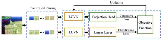
Figure 1. The framework of the proposed LCVSNet.

2.1. The Lightweight Complex-Valued Network

This section details the LCVN, which consists of scattering and spatial modules, as illustrated in Figure 2. The design of both modules is driven by two lightweight strategies. Specifically, the scattering module reduces complexity by replacing 3D convolutions with efficient 1D convolutions along the scattering dimension (Section 2.1.1), while the spatial module adopts efficient cheap operations to expand features with a lower cost (Section 2.1.2). Section 2.1.3 provides a theoretical analysis of the achieved reduction in floating-point operations (FLOPs) and parameters (Params).

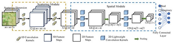
Figure 2. Architecture of the LCVN. LCVN primarily consists of a scattering module and a spatial module. In the scattering module, 1D convolution kernels in the scattering dimension are used to capture scattering features. In the spatial module, 2D lightweight convolutions are designed to extract rich spatial information. At last, the real and imaginary elements of the extracted features are used for classification.

2.1.1. Simple Scattering Module

For LCVN, the scattering module is used to capture the inter-element dependencies of polarimetric coherency matrix. The input of LCVN is represented as $x\in {\mathbb{C}}^{M\times M\times C}$, where M is the width and height of the sample, $\mathbb{C}$ represents the CV domain, and $C=6$ denotes the six elements of coherency matrix, i.e., $[T_{11},T_{12},T_{13},T_{22},T_{23},T_{33}]$. For the first convolution layer, $N_1$ convolution kernels $w\in {\mathbb{C}}^u$ perform convolution operations on the input along the scattering dimension to obtain the output O, which can be expressed by

$$\begin{array}{cc}\hfill O_k^{\mathrm{abc}}& =\mathbb{C}\mathrm{ReLU}\left(V_k^{\mathrm{abc}}\right)=\mathrm{ReLU}\left(\Re \left(V_k^{\mathrm{abc}}\right)\right)+\mathrm{j}\mathrm{ReLU}\left(\Im \left(V_k^{\mathrm{abc}}\right)\right)\hfill \\ \hfill V_k^{\mathrm{abc}}& =\sum _{r=1}^u\left(\Re \left(w_k^r\right)\ast \Re \left(x^{\mathrm{ab}\left(\mathrm{c}+r-1\right)}\right)-\Im \left(w_k^r\right)\ast \Im \left(x^{\mathrm{ab}\left(\mathrm{c}+r-1\right)}\right)\right)\hfill \\ \hfill & +\mathrm{j}\sum _{r=1}^u\left(\Re \left(w_k^r\right)\ast \Im \left(x^{\mathrm{ab}\left(\mathrm{c}+r-1\right)}\right)+\Im \left(w_k^r\right)\ast \Re \left(x^{\mathrm{ab}\left(\mathrm{c}+r-1\right)}\right)\right)\hfill \\ \hfill & +\Re \left(b_k\right)+\mathrm{j}\Im \left(b_k\right).\hfill \end{array}$$

(1)

where $V_k^{\mathrm{abc}}$ represents the value of the kth feature map at coordinate $\left(\mathrm{a},\mathrm{b},\mathrm{c}\right)$, u is the size of 1D convolution kernels, * represents the convolution operation, $\Re \left(·\right)$ and $\Im \left(·\right)$ refer to the real and imaginary components of the complex numbers respectively, $\mathrm{j}=\sqrt{-1}$ represents the imaginary unit, $b_k$ represents bias, and $\mathbb{C}\mathrm{ReLU}$ represents the rectified linear unit (ReLU) activation function operating in the CV domain.

The second convolution layer of the scattering module further integrates the scattering information of polarimetric data and converts the feature maps from 3D to 2D, which can be given by

$$\begin{array}{cc}\hfill V_k^{\mathrm{ab}}& =\sum _{i=1}^{N_1}\sum _{r=1}^C\left(\Re \left(w_{ki}^r\right)\ast \Re \left(O_i^{\mathrm{ab}r}\right)-\Im \left(w_{ki}^r\right)\ast \Im \left(O_i^{\mathrm{ab}r}\right)\right)\hfill \\ \hfill & +\mathrm{j}\sum _{i=1}^{N_1}\sum _{r=1}^C\left(\Re \left(w_{ki}^r\right)\ast \Im \left(O_i^{\mathrm{ab}r}\right)+\Im \left(w_{ki}^r\right)\ast \Re \left(O_i^{\mathrm{ab}r}\right)\right)\hfill \\ \hfill & +\Re \left(b_k\right)+\mathrm{j}\Im \left(b_k\right).\hfill \end{array}$$

(2)

This design serves as a lightweight alternative to a standard 3D CV convolution. By focusing solely on the scattering dimension, it significantly reduces the computational costs while effectively capturing the inherent dependencies within the coherency matrix. A detailed theoretical analysis of the achieved cost reduction is provided in Section 2.1.3.

2.1.2. Lightweight Spatial Module

Following the extraction of scattering features, the spatial module is designed to capture contextual information from neighboring pixels. However, a direct application of standard 2D CV convolutions would be computationally expensive. Its lightweight architecture is motivated by a key observation from our preliminary experiments on a simulated PolSAR dataset [19,37]. As shown in Figure 3, there are some redundant feature maps with similar structures but different intensities. It is unnecessary to use a large number of computational resources to learn these redundant feature maps. Assuming that a set of intrinsic feature maps is generated by a relatively small number of convolution kernels, rich feature maps can be obtained by performing cheap operations on the intrinsic features [38]. Based on this assumption, we design the lightweight CV convolution shown in Figure 4. This design generates the majority of output feature maps through inexpensive depthwise convolutions, thereby achieving richer feature representations at a lower computational cost.

Figure 3. Visualization of the features learned by the CVCNN on a simulated image. (a) Pauli RGB of the simulated image. (b) Feature maps extracted by the CVCNN from the red box region in Figure 3a. In order to visualize the CV features, we take the absolute value of the features. The blue denotes zero, and the other colors represent non-zero.

Figure 4. Architecture of the proposed lightweight CV convolution. It reduces computational costs by using a primary convolution to generate a small set of intrinsic features, which are then efficiently expanded into a full set of feature maps through cheap operations. Finally, a skip connection preserves input information.

The lightweight CV convolution is constructed as follows. First of all, $N_d^l$ convolution kernels $w^l\in {\mathbb{C}}^{u\times u\times N_i^l}$ are applied to the features of the previous layer $O_o^{\left(l-1\right)}$, which can be expressed as

$$\begin{array}{cc}\hfill V_k^l& =\sum _{i=1}^{N_i^l}\left(\Re \left(w_{ki}^l\right)\ast \Re \left(O_o^{\left(l-1\right)}\right)-\Im \left(w_{ki}^l\right)\ast \Im \left(O_o^{\left(l-1\right)}\right)\right)\hfill \\ \hfill & +\mathrm{j}\sum _{i=1}^{N_i^l}\left(\Re \left(w_{ki}^l\right)\ast \Im \left(O_o^{\left(l-1\right)}\right)+\Im \left(w_{ki}^l\right)\ast \Re \left(O_o^{\left(l-1\right)}\right)\right)\hfill \\ \hfill & +\Re \left(b_k^l\right)+\mathrm{j}\Im \left(b_k^l\right).\hfill \end{array}$$

(3)

Then, $F^l$ is obtained by performing CV activation $\mathbb{C}\sigma (·)$ on $V^l$. Second, a series of cheap operations are conducted on the intrinsic features $F^l$ to generate S ghost features, and the formula can be expressed as

$$g_{sk}^l={\mathrm{\Phi }}_{sk}\left(F_k^l\right),\forall k=1,\dots ,N_d^l,s=1,\dots ,S$$

(4)

where ${\mathrm{\Phi }}_s\left(·\right)$ represents a depthwise convolution (i.e., cheap operation), and S denotes the number of cheap operations. In particular, when $s=S$, the cheap operation is an identity mapping. In this way, at this stage, $N_d^l·S$ feature maps $G=\left[g_{11}^l,g_{12}^l,\dots ,g_{N_d^l·S}^l\right]$ are obtained. Furthermore, the features $O_o^{\left(l-1\right)}$ and ghost features are concatenated by skip connection, as shown in Figure 4, which preserves the information of previous layers. In this way, the number of output feature maps is $N_o^l=N_d^l·S+N_i^l$, where $N_i^l$ denotes the dimension of the input features to the l-th 2D lightweight convolution layer. Importantly, compared to the primary convolution with the same number of convolution kernels, the lightweight convolution enriches the feature representation through the cheap operation and the skip connection while significantly reducing the computational complexity and the number of parameters. After each lightweight convolution layer, a pooling layer follows to reduce the feature size and improve the generalization of the features.

2.1.3. Lightweight Analysis

To quantify and validate the efficiency of the proposed lightweight design, we conduct a theoretical analysis of the required FLOPs and Params. In this analysis, we assume that the nonlinear activation is computed for free, and each multiplication or addition is counted as one FLOP. For real-valued (RV) convolution, Params is computed by

$${\mathrm{P}}_{\mathrm{RVC}}=\left(u^2\times N_i^l+1\right)\times N_o^l.$$

(5)

The corresponding FLOPs are given by

$$\begin{array}{cc}\hfill {\mathrm{F}}_{\mathrm{RVC}}& =\left[\left(u^2\times N_i^l\right)+\left(u^2\times N_i^l-1\right)+1\right]\times N_o^l\times h^l\times w^l\hfill \\ \hfill & =2u^2\times N_i^l\times N_o^l\times h^l\times w^l\hfill \end{array}$$

(6)

where $\left\{w^l,h^l\right\}$ denotes the width and height of the output features, respectively.

According to Equation (3), one CV convolution involves four RV convolution operations and two elementwise addition operations. In this way, the Params and FLOPs of CV convolution are expressed as

$${\mathrm{P}}_{\mathrm{CVC}}=\left(u^2\times N_i^l+1\right)N_o^l$$

(7)

$$\begin{array}{cc}\hfill {\mathrm{F}}_{\mathrm{CVC}}& =\left[\left(N_i^l\times u^2\right)+\left(N_i^l\times u^2-1\right)+1\right]\times 4\times w^l\times h^l\times N_o^l\hfill \\ \hfill & +2\times w^l\times h^l\times N_o^l\hfill \\ \hfill & =\left(2N_i^l\times u^2\times 4+2\right)\times w^l\times h^l\times N_o^l\hfill \end{array}$$

(8)

Our 2D lightweight CV convolution involves two main components: primary convolutions and cheap operations. Thus, the Params and FLOPs of lightweight CV convolution are given by

$$\begin{array}{cc}\hfill {\mathrm{P}}_{\mathrm{LCVC}}& =\left(u^2\times N_i^l+1\right)\times N_d^l\hfill \\ \hfill & +\left(S-1\right)\times \left(d^2+1\right)\times N_d^l\hfill \end{array}$$

(9)

$$\begin{array}{cc}\hfill & {\mathrm{F}}_{\mathrm{LCVC}}=\left(2N_i^l\times u^2\times 4+2\right)\times N_d^l\times w^l\times h^l\hfill \\ \hfill & +\left(2\times d^2\times 4+2\right)\times N_d^l\times \left(S-1\right)\times w^l\times h^l\hfill \end{array}$$

(10)

where the first term in ${\mathrm{P}}_{\mathrm{LCVC}}$ and ${\mathrm{F}}_{\mathrm{LCVC}}$ refers to the primary convolution, the second term refers to the cheap operation, d is the kernel size of the cheap operation, and $N_d^l=\left(N_o^l-N_i^l\right)/S$.

In our model, d and S are set to 3 and 2, respectively. We have

$$\begin{array}{cc}\hfill r_{{\mathrm{P}}_l}& ={\displaystyle \frac{{\mathrm{P}}_{\mathrm{LCVC}}}{{\mathrm{P}}_{\mathrm{CVC}}}}\hfill \\ \hfill & ={\displaystyle \frac{N_o^l-N_i^l}{N_o^{l}S}}+{\displaystyle \frac{S-1}{S}}\times {\displaystyle \frac{d^2+1}{u^2{N}_i^l+1}}\times {\displaystyle \frac{N_o^l-N_i^l}{N_o^l}}\hfill \\ \hfill & ={\displaystyle \frac{1}{4}}+{\displaystyle \frac{1}{4}}\times {\displaystyle \frac{d^2+1}{u^2{N}_i^l+1}}\hfill \end{array}$$

(11)

$$\begin{array}{cc}\hfill r_{{\mathrm{F}}_l}& ={\displaystyle \frac{{\mathrm{F}}_{\mathrm{LCVC}}}{{\mathrm{F}}_{\mathrm{CVC}}}}\hfill \\ \hfill & ={\displaystyle \frac{N_o^l-N_i^l}{N_o^l·S}}+{\displaystyle \frac{S-1}{S}}·{\displaystyle \frac{4d^2+1}{4N_i^l{u}^2+1}}·{\displaystyle \frac{N_o^l-N_i^l}{N_o^l}}\hfill \\ \hfill & ={\displaystyle \frac{1}{4}}+{\displaystyle \frac{1}{4}}·{\displaystyle \frac{4d^2+1}{4N_i^l{u}^2+1}}\hfill \end{array}$$

(12)

Thus, $1/4<r_{{\mathrm{P}}_l}\le 1/2$, and $1/4<r_{{\mathrm{F}}_l}\le 1/2$. Furthermore, due to the similar ability to capture scattering information, the 3D CV convolution is compared to our simple scattering convolution. Similar to Equations (11) and (12), $r_{\mathrm{Ps}}={\mathrm{P}}_{1\mathrm{DC}}/{\mathrm{P}}_{3\mathrm{DC}}=1/u^2$, and $r_{\mathrm{Fs}}={\mathrm{F}}_{1\mathrm{DC}}/F_{3\mathrm{DC}}=1/u^2$. In summary, the proposed LCVN achieves a substantial decrease in computational costs through the synergistic effect of its two core modules. Theoretical analyses confirm that the scattering module reduces the Params and FLOPs required for capturing scattering dependencies to $1/u^2$ of those needed by a standard 3D CV convolution. Concurrently, the spatial module employing the lightweight CV convolution achieves a reduction ratio of $r_{P_l}$ and $r_{F_l}$ between $1/4$ and $1/2$ for Params and FLOPs, respectively, compared to its standard counterpart. Therefore, in LCVN, the two lightweight strategies, which employ the efficient 1D CV scattering convolutions together with the lightweight 2D CV spatial convolutions, constitute the principal technical pathway for achieving a substantial decrease in computational costs.

2.2. Lightweight Complex-Valued Siamese Network

Based on the LCVN, we propose LCVSNet, as shown in Figure 5, a Siamese network designed specifically for few-shot PolSAR image classification. The framework achieves robust classification with limited labels by integrating supervised contrastive learning directly into the training process. Our method explicitly uses the available labeled samples to construct sample pairs through a controlled pairing strategy. These positive and negative sample pairs, composed of similar and dissimilar patches, are fed into two weight sharing LCVN branches. Their outputs are then mapped through a projection head where a contrastive loss is applied to pull together features from the same class and push apart those from different classes. Simultaneously, the same extracted features are directed to a linear classifier supervised by a cross-entropy loss. The two losses are jointly optimized so that the network learns a feature space that is both discriminative and generalizable from very few labeled samples. After training, the Siamese structure is streamlined for inference. Specifically, only a single LCVN branch together with the linear classifier is preserved, allowing efficient and accurate classification of new PolSAR patches without requiring pairwise comparisons. Thus, LCVSNet effectively transforms contrastive learning into a few-shot supervised paradigm that amplifies the utility of limited labels.

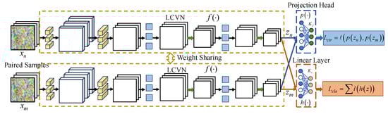
Figure 5. Backbone of LCVSNet. A pair of samples $\left\{x_n,x_m\right\}$ is fed into two LCVNs with weight sharing to extract deep features $\left\{z_n,z_m\right\}$, where $z=f\left(x\right)$. Then, the extracted deep features are fed into a projection head and a linear layer to compute the similarity comparison loss $L_{ctr}$ and classification loss $L_{cla}$. Finally, the network is jointly optimized by the two losses.

2.2.1. Controlled Pairing Strategy

The Siamese network augments the training set by pairing samples. Positive samples represent pairs of patches cropped from homogeneous regions, and negative samples denote pairs of patches cropped from heterogeneous regions. Assuming that the number of categories is $K_c$ and the number of samples per class is N. Thus, there are $N\times \left(N-1\right)/2\times K_c$ positive samples and $N^2\times \left(K_c-1\right)\times K_c/2$ negative samples. The proportion of positive samples to negative samples is approximately $1:\left(K_c-1\right)$. As a result, the larger the number of categories, the larger the proportion of negative samples. Although more negative samples can augment the training set, too many negative samples can significantly increase training time and negatively impact the network. To reasonably augment samples, the proportion of positive samples to negative samples is empirically controlled to be $1:2$. In our model, the training set comprises all positive samples along with randomly selected negative samples without replacement.

2.2.2. Projection Head

$X={\left\{x_n\in {\mathbb{C}}^{M\times M\times C}\right\}}_{n\in \left\{1,\dots ,N\right\}}$ denotes the patches cropped from PolSAR images, and $Y={\left\{y_n\in \mathrm{\Omega }\right\}}_{n=\left\{1,\dots ,N\right\}}$ is their labels, where $\mathrm{\Omega }$ is the set of $K_c$ one-hot codes denoting $K_c$ different labels. The LCVN is an encoder denoted by the function f, and $z=f\left(x\right)$ represents the extracted features. The projection head and the linear layer are represented by the function p and h, respectively.

The projection head is a fully connected layer, which prevents z from changing drastically to meet the needs of CL. Compared to the direct optimization of $z=f\left(x\right)$ with contrastive loss, the introduction of the projection head improves the generalization of features z, facilitating classification. Some researchers have demonstrated its ability to prevent information loss due to contrastive loss [39,40].

2.2.3. Objective Function

The objective function of the network consists of the contrastive loss $L_{ctr}$ and classification loss $L_{cla}$, which is expressed as

$$L=L_{ctr}+L_{cla}$$

(13)

With the Adam optimizer, the optimal network parameters can be trained by jointly optimizing the objective function. Concretely, there are two stages in each training epoch, including CL and classification optimization. First, the network is optimized by the contrastive loss $L_{ctr}$

$$L_{ctr}=t_{mn}{D}^2+\left(1-t_{mn}\right){\left\{\max \left(0,\alpha -D\right)\right\}}^2$$

(14)

$$D={∥p\left(z_m\right)-p\left(z_n\right)∥}_2$$

(15)

When $\left(x_m,x_n\right)$ contains positive samples, $t_{mn}=1$; otherwise, $t_{mn}=0$. D represents the distance between different samples, and $\alpha >0$ is a predefined margin controlling the degree of discrimination. By minimizing the contrastive loss, the extracted features have smaller intra-class distances and larger inter-class distances.

After CL, the cross-entropy loss is utilized to fine-tune the network parameters for classification, and the expression is given by

$$L_{cla}=\sum _{n=1}^N{y}_{n}log\left(h\left(z_n\right)\right)$$

(16)

After many epochs, the learned features have stronger representation abilities, which improves the PolSAR image classification performance even using a few labeled samples.

3. Results

3.1. Data

We evaluated the performance of the model on three datasets: San Francisco, Flevoland, and GF3 San Francisco. The details of each are as follows.

(1)

San Francisco dataset: The San Francisco dataset ($900\times 1024$) was acquired in 1989 by L-band AIRSAR over San Francisco Bay, USA. It covers five terrain classes: high-density urban, vegetation, water, developed urban, and low-density urban. The Pauli RGB image and ground truth are shown in the subsequent classification results.

(2)

Flevoland dataset: The Flevoland dataset was acquired by L-band AIRSAR over Flevoland, Netherlands, in 1989, and its size is $750\times 1024$. It contains 15 terrain classes: stembeans, peas, forest, lucerne, wheat, beet, potatoes, bare soil, grasses, rapeseed, barley, wheat2, wheat3, water, and buildings. The Pauli RGB image and ground truth are shown in the subsequent classification results.

(3)

GF3 San Francisco dataset: The GF3 San Francisco dataset was acquired by C-band Gaofen-3 over San Francisco Bay, in August 2018, whose size is $1800\times 1969$. There are five classes in this dataset: high-density urban, vegetation, water, developed urban, and low-density urban. The Pauli RGB image and ground truth are shown in the subsequent classification results. The ground truth map is manually annotated based on the Pauli RGB image and contemporaneous high-resolution Google Map.

In a PolSAR image, each pixel is represented by a six-dimensional covariance matrix, denoted as $\left[T_{11},T_{12},T_{13},T_{22},T_{23},T_{33}\right]$ [34]. A large-scale PolSAR image is partitioned into overlapping patches of size $n^{\prime }\times n^{\prime }\times 6$ using a sliding window, where $n^{\prime }$ is the neighborhood size. These patches serve as the network input.

3.2. Parameter Setting

There are several key parameters that need to be preset. The network is trained for 60 epochs, with the mini-batch size set to 64 in each epoch. The learning rates for CL and classification are $5\times {10}^{-5}$ and $1\times {10}^{-3}$, respectively. The projection head outputs 32-dimensional vectors without activation functions. In our model, the number of cheap operations S is set to 2. When $s=1$, it implements depthwise convolutions with a kernel size of 3 and $\mathbb{C}\mathrm{ReLU}$ activation, while $s=2$ represents an identity mapping. The margin $\alpha$ in the contrastive loss is set to 0.8. The rectified linear unit (ReLU) is used as the activation function.

3.3. Comparison Models

There are six other comparison models: (1) Wishart classification (WC) [41]; (2) CV3DCNN [34]; (3) CV-MsAtVit [42]; (4) S3Net [43]; (5) 3D convolutional Siamese network (3DCSN) [40]; (6) S2TNet [44]. The WC is a classic method for PolSAR classification. The remaining five models are all capable of extracting scattering and spatial information from PolSAR data. CV3DCNN extracts deep features in the spatial and scattering dimensions of PolSAR data using 3D CV convolution and is a representative CV network for PolSAR image classification. CV-MsAtVit employs a triple-branch parallel architecture to independently extract spatial features, scattering features, and scattering-spatial interaction features. These features are then fused through cascaded a CV attention block and CV-Vit to capture scattering and spatial information more completely. For these two models, each pixel of the input is the CV coherency matrix T. S3Net, 3DCSN, and S2TNet adopt lightweight RV network architectures and CL schemes for few-shot image classification, whose inputs are the real vector [$T_{11}$,$\Re \left(T_{12}\right)$, $\Im \left(T_{12}\right)$, $\Re \left(T_{13}\right)$, $\Im \left(T_{13}\right)$, $T_{22}$, $\Re \left(T_{23}\right)$, $\Im \left(T_{23}\right)$, $T_{33}$] consisting of the real and imaginary elements of the coherency matrix T. In addition, we separately present the results of our LCVN to demonstrate the effectiveness of this specific structure.

3.4. Experiment on the San Francisco

To visually analyze the ability of different models to represent polarimetric SAR scattering characteristics, we employed t-SNE [45,46] to visualize the features of 500 samples in a 2D Euclidean space (Figure 6). In the original feature space, different land cover categories exhibit severe overlap and ambiguous boundaries (Figure 6a), reflecting the classification challenges posed by overlapping scattering mechanisms. Although CV3DCNN exhibits a certain level of class separation (Figure 6b), model overfitting leads to confusion in scattering features between high-density urban (red) and developed urban (yellow) areas, as well as between vegetation (green) and low-density urban (purple) areas. By employing parallel architectures to extract multi-scale scattering and spatial features, CV-MsAtVit achieves more comprehensive information extraction (Figure 6c), demonstrating better discrimination between high-density urban (red) and developed urban (yellow) areas. However, due to insufficient labeled samples, feature overlap occurs between water (blue) and vegetation (green) areas. S3Net, 3DCSN, and S2TNet enhance intra-class consistency through feature similarity constraints. Among them, S3Net (Figure 6d) and S2TNet (Figure 6f) exhibit compact intra-class distributions but insufficient inter-class differences. While 3DCSN (Figure 6e) increases the inter-class distance, significant overlap remains in scattering features between easily confusable categories such as vegetation and low-density urban areas. Compared to CV3DCNN and CV-MsAtVit using identical training mechanisms, our lightweight CV network maintains superior performance with significantly fewer parameters, even when trained with extremely limited labeled samples, as shown in Figure 6g. Furthermore, the proposed LCVSNet introduces a projection head for CL, extracting features that exhibit not only highly separable cluster centers but also minimal inter-class overlap (Figure 6h). Fortunately, through joint optimization of contrastive and classification losses, the intermediate features z (Figure 6i) demonstrate more compact intra-class distributions and more distinct inter-class separation compared to those extracted by LCVN, effectively balancing the advantages observed in both Figure 6g,h. This outcome confirms that the proposed method significantly enhances feature discriminability by explicitly capturing differences in scattering mechanisms.

Figure 6. T-SNE visualization of the San Francisco. (a) Original features. (b) CV3DCNN. (c) CV-MsAtVit. (d) S3Net. (e) 3DCSN. (f) S2TNet. (g) LCVN. (h) Head features of LCVSNet. (i) Middle features of LCVSNet.

Figure 7 presents the overall classification results. For the traditional WC method (see Figure 7c), a significant amount of misclassification is observed in vegetation and high-density urban areas. In the case of CV3DCNN (see Figure 7d), its extensive parameters lead to overfitting under limited supervision, resulting in poor performance. CV-MsAtVit utilizes a multi-scale fusion mechanism to capture richer scattering and spatial features, leading to more accurate classification as shown in Figure 7e. S3Net, 3DCSN, and S2TNet employ lightweight architectures to extract deep features while incorporating CL for few-shot classification, which alleviates overfitting and obtains good results, as shown in Figure 7f–h. Both S3Net and S2TNet show superior classification performance for developed and low-density urban areas but produce some misclassifications in water regions. 3DSCN model achieves relatively accurate results, despite some misclassification of high-density urban areas in developed urban regions. However, these models are designed for hyperspectral images and exhibit limited capability in capturing polarimetric information. Our LCVN, specifically designed for CV PolSAR data, has fewer parameters and can accurately classify different terrains even with a small number of labeled samples. Furthermore, by optimizing both contrastive loss and classification loss, our LCVSNet reduces the misclassifications in vegetation and developed urban areas, obtaining more precise classification results, as shown in Figure 7j.

Figure 7. Classification results of the San Francisco. (a) Pauli RGB. (b) Ground truth. (c) WC (d) CV3DCNN. (e) CVMsAtVit. (f) S3Net. (g) 3DCSN. (h) S2TNet. (i) LCVN. (j) LCVSNet.

Table 1 lists the quantitative evaluation for the San Francisco dataset, where the five classes are ordered as: (1) high-density urban, (2) vegetation, (3) water, (4) developed urban, and (5) low-density urban. The traditional WC model fails to classify the San Francisco dataset effectively. CV3DCNN and CV-MsAtVit, optimized solely by classification loss, achieve poor results when the number of samples is small, with accuracies of 85.44% and 86.83%, respectively. S3Net, 3DCSNet, and S2TNet are networks jointly trained using contrastive loss and classification loss, and they achieve high classification accuracy in high-density urban (Class1) areas. In particular, 3DCSNet achieves the highest classification accuracy in low-density urban regions. However, the three RV networks cannot utilize the amplitude and phase information of PolSAR data. LCVNet comprehensively extracts scattering and spatial features and jointly optimizes the network parameters using contrastive and classification losses. The extracted deep features are discriminative and robust. As a result, LCVNet demonstrates superior performance, achieving an OA of 93.11% and a Kappa coefficient of 0.9035.

Table 1. Quantitative Evaluation of the San Francisco.

Class	Class1	Class2	Class3	Class4	Class5	OA	Kappa
WC	60.30%	59.02%	98.69%	85.50%	70.29%	79.66%	0.7191
CV3DCNN	82.62%	65.64%	98.49%	80.93%	83.33%	85.44%	0.7987
CV-MsAtVit	87.65%	72.40%	96.46%	89.66%	88.37%	88.33%	0.8376
S3Net	94.90%	67.23%	93.65%	90.58%	78.35%	87.51%	0.8259
3DCSN	95.80%	79.75%	98.24%	78.08%	91.89%	91.01%	0.8740
S2TNet	91.01%	72.10%	95.69%	86.96%	92.64%	88.38%	0.8386
LCVN	91.83%	77.53%	98.64%	86.96%	87.54%	90.91%	0.8726
LCVSNet	90.39%	87.32%	98.97%	89.43%	82.74%	93.11%	0.9035

3.5. Experiment on the Flevoland

Figure 8 shows the t-SNE visualization results of features extracted from the Flevoland by various models, with 500 samples per class. As shown in Figure 8a, the original feature points are clustered into two clusters and overlap each other, indicating limited discriminability. Both CV3DCNN and CV-MsAtVit (Figure 8b,c) achieve partial separation of features, but some overlap persists due to insufficient labeled samples. In comparison, S3Net, 3DCSN, and S2TNet incorporate joint optimization of classification and contrastive loss. The inclusion of CL enhances feature discrimination, as visibly reduced overlap in Figure 8d–f demonstrates. Among them, 3DCSN achieves the most distinct feature separation. This is attributed to its projection head, which directly optimizes features for CL. Inspired by this, we propose the LCVN with significantly reduced parameters. This design not only lowers computational costs but also improves performance with a small number of samples. Figure 8g confirms that LCVN achieves clearer feature separation than both CV3DCNN and CV-MsAtVit. Furthermore, the projection features $p\left(z\right)$ as shown in Figure 8h exhibit compact intra-class and dispersed inter-class distributions. Finally, Figure 8i shows that features z effectively combine the strengths of Figure 8g,h. With the projection head, features z can meet CL requirements with minimal changes, preserving information critical for classification.

Figure 8. T-SNE visualization of the Flevoland. (a) Original features. (b) CV3DCNN. (c) CV-MsAtVit. (d) S3Net. (e) 3DCSN. (f) S2TNet. (g) LCVN. (h) Head features of LCVSNet. (i) Middle features of LCVSNet.

Figure 9 and Figure 10 presents the classification results. Generally, WC, CV3DCNN, S3Net, and S2TNet exhibit limited robustness to speckle, whereas 3DCSN struggles with accurate terrain classification. Due to the greater number of categories in the Flevoland dataset, the overall quantity of samples alleviates the label scarcity problem. As a result, CV3DCNN, CV-MsAtVit, and LCVN demonstrate competent terrain identification capabilities, as evidenced in Figures: We revised the citation format. Please check them carefully. Figure 9c and Figure 10c, Figure 9d and Figure 10d, and Figure 9h and Figure 10h. S3Net, 3DCSN, and S2TNet employ feature similarity constraints to enhance discriminative feature extraction. However, as RV networks, they cannot fully utilize the phase information in polarimetric data, leading to noticeable misclassifications, such as forest areas in Figure 9e and Figure 10e, water areas in Figure 9f and Figure 10f, and stembeans areas in Figure 9g and Figure 10g. Our LCVN incorporates not only amplitude and phase information but also the scattering information between multiple channels of polarimetric data. Notably, its well-designed lightweight architecture promotes more efficient utilization of limited samples, obtaining superior classification, as shown in Figure 9h and Figure 10h. By employing a contrastive loss in the Siamese architecture, LCVSNet further improves the discrimination of features. As a result, the wheat and rapeseed areas disturbed by wheat2 are correctly classified, as shown in Figure 9i and Figure 10i.

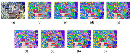
Figure 9. Classification results of the Flevoland. (a) Pauli RGB. (b) WC (c) CV3DCNN. (d) CV-MsAtVit. (e) S3Net. (f) 3DCSN. (g) S2TNet. (h) LCVN. (i) LCVSNet.

Figure 10. Classificationresults overlaid on the ground truth for the Flevoland. (a) Ground truth. (b) WC. (c) CV3DCNN. (d) CV-MaAtVit. (e) S3Net. (f) 3DCSN. (g) S2TNet. (h) LCVN. (i) LCVSNet.

The quantitative results are presented in Table 2. The Flevoland dataset contains 15 different terrains, and the total number of samples alleviates the overfitting problem. Thus, the deep learning methods exhibit higher overall accuracy than the traditional WC method. CV3DCNN and CV-MsAtVit, specifically designed for PolSAR images, achieve high classification accuracy. Neither S3Net nor S2TNet can fully utilize phase information, resulting in limited classification accuracy (70.71% for S3Net in forest areas and 60.76% for S2TNet in the stembeans areas), consistent with Figure 9e,g. 3DCSN exhibits similar limitations, demonstrating relatively low accuracy in wheat areas (77.72%) and rapeseed areas (76.04%) compared to other models. By comprehensively leveraging amplitude, phase, and scattering characteristics of polarimetric data, the LCVN obtains satisfying results with its OA being 95.77% and Kappa being 0.8783. Furthermore, our LCVSNet, a Siamese network of the LCVN, introduces additional CL to enhance feature discrimination. After fine-tuning with limited samples, it achieves classification accuracies of 98.65% in wheat areas and 94.23% in water areas. LCVSNet demonstrates superior performance with its OA surpassing CV3DCNN, CV-MsAtVit, S3Net, 3DCSN, and S2TNet by 4.17%, 6.78%, 8.14%, 8.35%, and 8.26% respectively, while its Kappa coefficient shows corresponding improvements of 0.0455, 0.0736, 0.0887, 0.0908, and 0.0902 over these comparative models.

Table 2. Quantitative Evaluation of the Flevoland.

Class	WC	CV3DCNN	CV-MsAtVit	S3Net	3DCSN	S2TNet	LCVN	LCVSNet
1. Stembeans	95.40%	93.69%	98.31%	95.89%	94.45%	60.76%	99.07%	99.56%
2. Peas	95.13%	95.96%	94.96%	92.62%	87.15%	90.96%	97.65%	98.87%
3. Forest	85.27%	93.66%	95.22%	70.71%	96.16%	88.39%	99.57%	96.74%
4. Lucerne	93.87%	96.95%	96.67%	99.74%	94.91%	94.26%	97.88%	99.24%
5. Wheat	84.55%	94.97%	83.90%	83.49%	77.72%	91.07%	83.31%	98.65%
6. Beet	97.33%	96.88%	99.63%	93.95%	96.29%	90.46%	99.21%	99.45%
7. Potatoes	95.36%	83.33%	95.76%	82.47%	90.09%	80.78%	98.46%	98.23%
8. Bare soil	98.05%	98.44%	98.83%	1	87.26%	97.27%	1	95.91%
9. Grasses	68.38%	88.98%	88.87%	92.06%	98.77%	88.66%	97.69%	96.03%
10. Rapeseed	59.51%	84.20%	90.66%	88.64%	76.04%	85.15%	94.79%	96.64%
11. Barley	93.45%	96.66%	90.55%	91.17%	88.78%	85.69%	97.92%	99.97%
12. Wheat 2	85.90%	88.98%	94.49%	89.86%	94.33%	79.27%	99.29%	91.27%
13. Wheat 3	88.92%	94.73%	94.58%	91.32%	98.90%	97.37%	97.74%	96.75%
14. Water	55.99%	99.94%	57.70%	97.97%	69.39%	99.62%	89.54%	94.23%
15. Buildings	94.54%	98.11%	96.01%	93.70%	98.32%	1	1	99.16%
OA	84.35%	93.00%	90.39%	89.03%	88.82%	88.91%	95.77%	97.17%
Kappa	0.8297	0.9236	0.8955	0.8804	0.8783	0.8789	0.9539	0.9691

3.6. Experiment on the GF3 San Francisco

Figure 11 displays feature distributions with 500 samples per class. Compared to the original data (Figure 11a), both CV3DCNN and CV-MsAtVit enlarge the inter-class distance for the features of the green, purple, and pink categories. However, due to overfitting caused by insufficient labeled samples, their intra-class distributions remain dispersed, as shown in Figure 11b,c. Although S3Net, 3DCSN, and S2TNet extract deep features through joint contrastive and classification losses, their RV architecture cannot fully exploit the phase information of PolSAR data. As a result, overlap persists between purple and red clusters, as well as between green and pink clusters (Figure 11d–f). In comparison, our LCVN significantly enlarges the inter-class distances between these challenging categories while maintaining more compact intra-class structure (Figure 11g). Furthermore, through CL, the projected features $p\left(z\right)$ form five clearly separated and compact clusters (Figure 11h). The middle features z (Figure 11i) combine the advantages of both Figure 11g,h, obtaining tighter intra-class clustering than LCVN and fewer overlaps than the projected features. This demonstrates that the introduced projection head enhances the discriminability of features z.

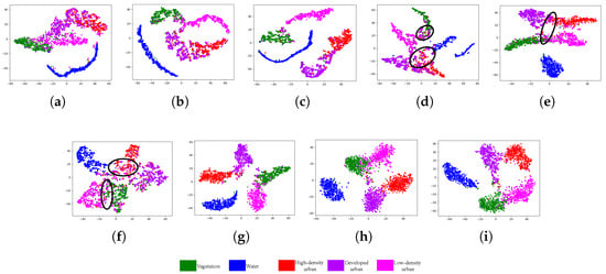
Figure 11. T-SNE visualization of the GF3 San Francisco dataset. (a) Original data. (b) CV3DCNN. (c) CV-MsAtVit. (d) S3Net. (e) 3DCSN. (f) S2TNet. (g) LCVN. (h) Head features of LCVSNet. (i) Middle features of LCVSNet.

Figure 12 shows the classification results. The traditional WC method achieves satisfactory result with a small number of samples, as shown in Figure 12c. Due to the insufficient number of labeled samples, CV3DCNN incorrectly labels a number of high-density urban areas in Figure 12d as developed ones. By utilizing a parallel multi-scale architecture to extract more scattering and spatial features, CV-MsAtVit achieves more accurate classification, particularly in the high-density urban areas, as shown in Figure 12e. However, its performance remains constrained by the limited labeled samples. S3Net and S2TNet fail to effectively utilize polarimetric information, leading to some misclassifications, as shown in Figure 12f,h. 3DCSN obtains accurate classification in water, vegetation, and developed urban regions, as shown in Figure 12g. Our LCVN faces difficulties in identifying vegetation areas when the number of labeled samples is small, as shown in Figure 12i. Compared to LCVN, LCVSNet introduces a Siamese structure and a projection head to enhance feature discrimination. As a result, the extracted deep features exhibit smaller intra-class distances and larger inter-class distances, which significantly improve classification performance. As shown in Figure 12j, our LCVSNet not only enhances terrain recognition accuracy but also achieves smoother classification results.

Figure 12. Classificationresults of the GF3 San Francisco. (a) Pauli RGB. (b) Ground truth. (c) WC. (d) CV3DCNN. (e) CV-MsAtVit. (f) S3Net. (g) 3DCSN. (h) S2TNet. (i) LCVN. (j) LCVSNet.

Table 3 lists their quantitative evaluations. As discussed previously, the developed urban and high-density urban classes are similar. Compared to the reference models that struggle with accurately identifying these two categories, our model demonstrates a significant advantage with OA being 97.06% and 92.43%, respectively. The relatively poor performance of S3Net and S2TNet on the GF3 San Francisco dataset can be attributed primarily to their inadequate extraction of polarimetric information. Similarly, although 3DCSN achieves high classification accuracy on datasets with fewer categories (such as the San Francisco and GF3 San Francisco datasets), its performance declines significantly on the more complex Flevoland dataset, which contains a larger number of categories. As a supervised model, our LCVN achieves high classification accuracy even with limited labeled samples, demonstrating the advantage of its lightweight structure. Building upon this, a CL output is incorporated to enhance feature discrimination, thus obtaining a higher accuracy, with an OA of 95.78% and a Kappa of 0.9385. Although data augmentation increases the training time of LCVSNet, its inference is efficient. In contrast to S3Net and S2TNet, which process multiple branches in parallel, our model operates in a single-branch mode during testing due to its weight sharing design. Consequently, LCVSNet achieves both high computational efficiency in inference and precise classification accuracy.

Table 3. Quantitative Evaluation of the GF3 San Francisco.

	WC	CV3DCNN	CV-MsAtVit	S3Net	3DCSN	S2TNet	LCVN	LCVSNet
Class1	89.91%	90.54%	90.54%	69.56%	91.16%	74.33%	71.55%	91.40%
Class2	99.45%	99.67%	98.86%	92.58%	99.75%	90.25%	99.61%	99.45%
Class3	61.26%	61.79%	91.46%	70.44%	79.78%	61.80%	95.57%	88.93%
Class4	80.32%	85.64%	74.87%	71.79%	91.98%	75.77%	93.71%	97.06%
Class5	69.01%	73.21%	81.14%	76.33%	87.99%	69.26%	92.43%	90.30%
OA	87.69%	88.98%	91.96%	81.69%	93.59%	80.19%	93.46%	95.78%
Kappa	0.8203	0.8385	0.8825	0.7376	0.9063	0.7173	0.9048	0.9385
Train (s)	2	3	5	8	137	2391	6	102
Test (s)		102	691	485	106	1276	216	179

4. Discussion

The results on the three PolSAR datasets comprehensively demonstrate the effectiveness of our model from three complementary perspectives: feature visualization, classification results, and quantitative evaluation. Based on the overall performance advantage of LCVSNet, we proceed to conduct a systematic analysis of its key influencing factors. Specifically, validation will be carried out from the following four aspects: (1) the impact of hyperparameter settings; (2) the effect of the number of training samples; (3) the effectiveness of the lightweight design. In addition, we quantify the computational costs of each model, highlighting the advantage of our approach in practical applications with limited hardware resources. Finally, we present the future work.

4.1. Hyperparameter Analysis

To investigate the impacts of two key hyperparameters (the neighborhood size and the number of training samples) on classification performance, we conducted experiments on the Flevoland and San Francisco datasets.

(1)

The neighborhood size: The experiment is set up to determine the neighborhood size. The influence of neighborhood size on classification accuracy is illustrated in Figure 13a, where the two lines denote the results for Flevoland and San Francisco, respectively. For the Flevoland dataset, classification accuracy tends to stabilize as the neighborhood size grows to 16. For the San Francisco dataset, peak classification accuracy is achieved with a neighborhood size of 16. As a result, the neighborhood size was fixed at 16.

Figure 13. Influence of neighborhood size and number of samples on classification accuracy based on two representative datasets. (a) Neighborhood size. (b) The number of samples. The number of samples for each class was 5, 10, 20, 40, 60, and 80.

(2)

The number of samples: The experiment is designed to determine the optimal number of samples. The influence of increasing the number of samples on classification accuracy is illustrated in Figure 13b. As the number of samples reaches 20, there is a rapid increase in classification accuracy, especially for the San Francisco dataset, which has a relatively small number of categories. To achieve higher classification accuracy with fewer samples, our experiments used 20 samples per class.

4.2. Effect of the Number of Samples

To evaluate the effect of different numbers of samples, we tested a varying number of samples on the San Francisco dataset, as shown in Figure 14. The WC method shows low overall performance. Although CV3DCNN and CVMsVit can simultaneously capture spatial and scattering information, their large number of parameters leads to overfitting with a small number of samples, resulting in poor classification performance. S3Net, 3DCSN, and S2TNet alleviate overfitting through concise architectures with fewer parameters and contrastive learning mechanisms. However, as these models are real-valued networks designed for real-valued images, they are difficult to fully exploit the phase and scattering information of complex-valued polarimetric data. Our LCVN overcomes these limitations through carefully designed lightweight CV convolution modules that significantly reduce the number of network parameters while improving classification performance with limited samples. Furthermore, LCVSNet combines the LCVN with the contrastive learning strategy, enhancing feature representation capabilities to achieve superior classification performance.

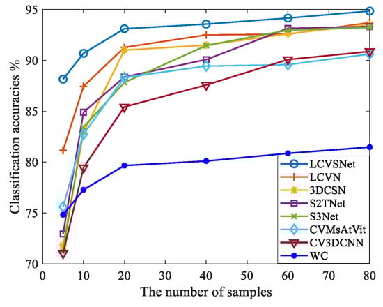
Figure 14. The effect of different number of samples on the classification performance. The number of samples for each class was 5, 10, 20, 40, 60, and 80.

4.3. Effectiveness of Lightweight Design

Table 4 presents several ablation models, including the CV Siamese network (CVSNet), 2D lightweight CV convolution removal (LCVCR), cheap operation removal (COR), and skip connection removal (SCR). These models were all based on a Siamese network architecture. They were designed by removing specific modules to form a comparative set for the purpose of validating the role of each module. All layers maintain a consistent number of output feature maps across these models for fair comparison. In the table, 1DCV Conv in the scattering module denotes 1D convolution applied along the scattering dimension. First, CVSNet serves as a baseline model functionally similar to ours, but with its scattering and spatial modules replaced by 3D CV convolution and primary CV convolution, respectively. Second, the 2D lightweight CV convolution incorporates two key lightweight operations, including the cheap operation (CO) and the skip connection (SC). To further evaluate the effectiveness of the two lightweight operations, we design additional experiments for the 2D lightweight CV convolution (LCVC). Specifically, we replaced the LCVC with primary CV convolution to demonstrate its overall impact. Then, we individually removed CO and SC from the LCVC to validate their contributions.

Table 4. Architectures of the ablation models.

	CVSNet	LCVCR	COR	SCR	LCVSNet
Scattering Module	3DCV Conv	1DCV Conv	1DCV Conv	1DCV Conv	1DCV Conv
	3DCV Conv	1DCV Conv	1DCV Conv	1DCV Conv	1DCV Conv
Spatial Module	2DCV Conv	2DCV Conv	2DCV Conv + SC	2DCV Conv + CO	2DCV Conv + CO + SC
	Pooling	Pooling	Pooling	Pooling	Pooling
	2DCV Conv	2DCV Conv	2DCV Conv + SC	2DCV Conv + CO	2DCV Conv + CO + SC
	Pooling	Pooling	Pooling	Pooling	Pooling

Table 5 shows the ablation study results on the effectiveness of lightweight design. Overall, the classification accuracies of different ablation models on the San Francisco dataset show minimal variation. However, both FLOPs and Params decrease gradually with the introduction of lightweight operations. For the Flevoland dataset, LCVSNet achieves superior accuracy with significantly reduced FLOPs and Params. Although CVSNet has a large number of parameters, it maintains high accuracy even with a small number of samples. This performance can be attributed to our dual-branch output structure and joint optimization mechanism. Compared to CVSNet, LCVC extracts scattering features by performing 1D CV convolutions along the scattering dimension rather than 3D CV convolutions, which greatly reduces both FLOPs and Params. Although LCVC is less effective than CVSNet in capturing spatial information, its simplified network structure facilitates accurate classification even with limited samples. In COR and SCR, some convolution operations are replaced by SC and CO, further reducing the FLOPs and Params. Since CO and SC can enrich feature representations, COR and SCR achieve comparable or even superior accuracy to LCVC. By incorporating CO and SC, our LCVSNet significantly reduces the computational complexity of the CV convolution network while maintaining high classification performance. Quantitatively, LCVC requires 2.6 times more FLOPs than LCVSNet. For the San Francisco and Flevoland datasets, LCVC contains 2.4 and 2.3 times more parameters than LCVSNet, respectively. These experimental results are consistent with the theoretical analysis presented in Section 2.1.3.

Table 5. Ablation study on the effectiveness of lightweight design.

OA	CVSNet	LCVCR	COR	SCR	LCVSNet
San Francisco	92.85%	91.77%	92.03%	92.35%	93.10%
Flevoland	95.28%	95.92%	95.01%	97.07%	97.17%
FLOPs (M)	CVSNet	LCVCR	COR	SCR	LCVSNet
San Francisco	100.4	45.3	26.3	26.9	17.1
Flevoland	100.4	45.3	26.3	26.4	17.1
Params (K)	CVSNet	LCVCR	COR	SCR	LCVSNet
San Francisco	336.1	236.3	143.5	145.4	98.1
Flevoland	346.4	246.5	153.8	155.7	108.3

4.4. Computational Costs Analysis

Section 4.3 verifies the theoretical analysis in Section 2.1.3 by comparing the FLOPs and Params of different ablation models. Here, we further extend the comparison to related models, as listed in Table 6, demonstrating the lightweight efficiency of our approach. CV3DCNN uses 3D CV convolutions to fully extract scattering and spatial features from PolSAR data, but it requires more FLOPs and Params. Specifically, for the San Francisco dataset, CV3DCNN requires 3.7 times the FLOPs and 19.0 times the parameters compared to LCVSNet. CV-MsAtVit employs multi-scale CV kernels and a lightweight CV attention module to extract scattering spatial features effectively while reducing FLOPs. However, its excessive parameters may limit performance in few-shot PolSAR image classification, as its parameter count is 30 times that of our LCVSNet. The results demonstrate that our model significantly reduces the computational costs of CV convolutional networks, including FLOPs and Params. Thus, our CV network requires fewer hardware resources in practical applications. In addition, the lower parameters promote the network to achieve better performance with fewer samples. Since a CV convolution requires four RV convolutions and two elementwise additions, RV convolution inherently has lower FLOPs. Despite this, LCVSNet still has fewer FLOPs and Params than RV S3Net, 3DCSN, and S2TNet. Specifically, 3DSCN requires 2 times the FLOPs and 12 times the Params of LCVSNet. The experimental results demonstrate that our LCVSNet can achieve few-shot classification with a lower computational cost, facilitating its practical deployment.

Table 6. Computational costs comparison.

Models	San Francisco		Flevoland
	FLOPs (M)	Params (K)	FLOPs (M)	Params (K)
CV3DCNN	63.0	1868.1	63.0	1869.4
CV-MsAtViT	16.9	2948.2	16.9	2958.5
S3Net	20.7	115.4	20.7	121.2
3DCSN	36.8	1256.0	36.8	1261.8
S2TNet	26.2	173.1	26.2	181.9
LCVN	17.1	65.3	17.1	75.5
LCVSNet	17.1	98.1	17.1	108.3

4.5. Future Work

Future work could explore integrating multi-source remote sensing data into the proposed framework. A cross-modal complex-valued Siamese architecture may further enhance both feature representation and generalization performance with extremely limited labeled samples.

5. Conclusions

A lightweight model called LCVSNet is proposed for few-shot PolSAR image classification. First, the LCVN was constructed, which combines the simple 1D CV convolution in the scattering dimension and the 2D CV lightweight convolution in the spatial dimension. Thus, the scattering spatial information of PolSAR was captured effectively at a lower computational cost. Then, a dual-output structure with a projection head for CL and a linear layer for classification was designed for LCVSNet, which enhances feature discrimination while preserving more useful information for classification. Experimental results have proved that our LCVSNet can accurately identify various terrains with a few labeled samples and lower computational resources.

References

- Lee, J.S.; Pottier, E. Polarimetric Radar Imaging: From Basics to Applications, 1st ed.; CRC Press: Boca Raton, FL, USA, 2009. [Google Scholar] [CrossRef]
- Yamaguchi, Y.; Moriyama, T.; Ishido, M.; Yamada, H. Four-component scattering model for polarimetric SAR image decomposition. IEEE Trans. Geosci. Remote Sens. 2005, 43, 1699–1706. [Google Scholar] [CrossRef]
- Mas, M.; Aguasca, A.; Broquetas, A.; Fàbregas, X.; Mallorqui Franquet, J.J.; Llop, J.; Lopez-Sanchez, J.M.; Kubanek, J. Facility for continuous agricultural field monitoring with a GB-PolSAR. IEEE J. Sel. Top. Appl. Earth Observ. Remote Sens. 2024, 17, 11866–11876. [Google Scholar] [CrossRef]
- Anconitano, G.; Lavalle, M.; Acuña, M.A.; Pierdicca, N. Sensitivity of polarimetric SAR decompositions to soil moisture and vegetation over three agricultural sites across a latitudinal gradient. IEEE J. Sel. Top. Appl. Earth Observ. Remote Sens. 2024, 17, 3615–3634. [Google Scholar] [CrossRef]
- Alkhatib, M.Q.; Zitouni, M.S.; Al-Saad, M.; Aburaed, N.; Al-Ahmad, H. PolSAR image classification using shallow to deep feature fusion network with complex valued attention. Sci. Rep. 2025, 15, 24315. [Google Scholar] [CrossRef] [PubMed]
- Shi, J.; Wang, W.; Jin, H.; Nie, M.; Ji, S. A lightweight Riemannian covariance matrix convolutional network for PolSAR image classification. IEEE Trans. Geosci. Remote Sens. 2024, 62, 4411017. [Google Scholar] [CrossRef]
- Li, F.; Yi, M.; Zhang, C.; Yao, W.; Hu, X.; Liu, F. PolSAR target recognition using a feature fusion framework based on monogenic signal and complex-valued nonlocal network. IEEE J. Sel. Top. Appl. Earth Observ. Remote Sens. 2022, 15, 7859–7872. [Google Scholar] [CrossRef]
- Shang, R.; Hu, M.; Feng, J.; Zhang, W.; Xu, S. A lightweight PolSAR image classification algorithm based on multi-scale feature extraction and local spatial information perception. App. Soft Comput. 2025, 170, 112676. [Google Scholar] [CrossRef]
- Wang, L.; Gui, R.; Hong, H.; Hu, J.; Ma, L.; Shi, Y. A 3-D convolutional vision Transformer for PolSAR image classification and change detection. IEEE J. Sel. Top. Appl. Earth Observ. Remote Sens. 2024, 17, 11503–11520. [Google Scholar] [CrossRef]
- Sun, Z.; Leng, X.; Zhang, X.; Zhou, Z.; Xiong, B.; Ji, K.; Kuang, G. Arbitrary-direction SAR ship detection method for multiscale imbalance. IEEE Trans. Geosci. Remote Sens. 2025, 63, 5208921. [Google Scholar]
- Sun, Z.; Leng, X.; Zhang, X.; Xiong, B.; Ji, K.; Kuang, G. Ship recognition for complex SAR images via dual-branch Transformer fusion network. IEEE Geosci. Remote Sens. Lett. 2024, 21, 4009905. [Google Scholar] [CrossRef]
- Zhou, Y.; Wang, H.; Xu, F.; Jin, Y.Q. Polarimetric SAR image classification using deep convolutional neural networks. IEEE Geosci. Remote Sens. Lett. 2016, 13, 1935–1939. [Google Scholar] [CrossRef]
- Dong, H.; Zhang, L.; Zou, B. PolSAR image classification with lightweight 3D convolutional networks. Remote Sens. 2020, 12, 396. [Google Scholar] [CrossRef]
- Wang, L.; Zhu, S.; Hong, H.; Shi, Y.; Zhu, Y.; Ma, L. WTC-HST: Wavelet transform convolutions and hierarchical spatial transformers for polarimetric SAR image classification. IEEE J. Sel. Top. Appl. Earth Observ. Remote Sens. 2025, 18, 21239–21253. [Google Scholar] [CrossRef]
- Song, W.; Liu, Q.; Pu, K.; Jiang, Y.; Wu, Y. Multiscale attention-enhanced complex-valued graph U-Net for PolSAR image classification. Remote Sens. 2025, 17, 3943. [Google Scholar] [CrossRef]
- Wang, Y.; Song, D.; Wang, W.; Rao, S.; Wang, X.; Wang, M. Self-supervised learning and semi-supervised learning for multi-sequence medical image classification. Neurocomputing 2022, 513, 383–394. [Google Scholar] [CrossRef]
- Bi, H.; Sun, J.; Xu, Z. A graph-based semisupervised deep learning model for PolSAR image classification. IEEE Trans. Geosci. Remote Sens. 2019, 57, 2116–2132. [Google Scholar] [CrossRef]
- Fang, Z.; Zhang, G.; Dai, Q.; Kong, Y.; Wang, P. Semisupervised deep convolutional neural networks using pseudo labels for PolSAR image classification. IEEE Geosci. Remote Sens. Lett. 2022, 19, 4005605. [Google Scholar] [CrossRef]
- Jiang, Y.; Li, M.; Zhang, P.; Song, W. Semisupervised complex network with spatial statistics fusion for PolSAR image classification. IEEE J. Sel. Top. Appl. Earth Observ. Remote Sens. 2023, 16, 9749–9761. [Google Scholar] [CrossRef]
- Yang, X.; Song, Z.; King, I.; Xu, Z. A survey on deep semi-supervised learning. IEEE Trans. Knowl. Data Eng. 2023, 35, 8934–8954. [Google Scholar] [CrossRef]
- Liu, X.; Zhang, F.; Hou, Z.; Mian, L.; Wang, Z.; Zhang, J.; Tang, J. Self-supervised learning: Generative or contrastive. IEEE Trans. Knowl. Data Eng. 2023, 35, 857–876. [Google Scholar] [CrossRef]
- Wang, N.; Jin, W.; Bi, H.; Xu, C.; Gao, J. A survey on deep learning for few-shot PolSAR image classification. Remote Sens. 2024, 16, 4632. [Google Scholar] [CrossRef]
- Zhang, L.; Zhang, S.; Zou, B.; Dong, H. Unsupervised deep representation learning and few-shot classification of PolSAR images. IEEE Trans. Geosci. Remote Sens. 2022, 60, 5100316. [Google Scholar] [CrossRef]
- Zhang, W.; Pan, Z.; Hu, Y. Exploring PolSAR images representation via self-supervised learning and its application on few-shot classification. IEEE Geosci. Remote Sens. Lett. 2022, 19, 4512605. [Google Scholar] [CrossRef]
- Qiu, W.; Pan, Z.; Yang, J. Few-shot PolSAR ship detection based on polarimetric features selection and improved contrastive self-supervised learning. Remote Sens. 2023, 15, 1874. [Google Scholar] [CrossRef]
- Dong, H.; Zhang, L.; Zou, B. Exploring vision transformers for polarimetric SAR image classification. IEEE Trans. Geosci. Remote Sens. 2022, 60, 5219715. [Google Scholar] [CrossRef]
- Chen, S.W.; Tao, C.S. PolSAR image classification using polarimetric-feature-driven deep convolutional neural network. IEEE Geosci. Remote Sens. Lett. 2018, 15, 627–631. [Google Scholar] [CrossRef]
- Zhang, L.; Chen, Z.; Zou, B.; Gao, Y. Polarimetric SAR terrain classification using 3D convolutional neural network. In Proceedings of the IGARSS— 2018 IEEE International Geoscience and Remote Sensing Symposium, Valencia, Spain, 22–27 July 2018; pp. 4551–4554. [Google Scholar] [CrossRef]
- Zhang, Z.; Wang, H.; Xu, F.; Jin, Y.Q. Complex-valued convolutional neural network and its application in polarimetric SAR image classification. IEEE Trans. Geosci. Remote Sens. 2017, 55, 7177–7188. [Google Scholar] [CrossRef]
- Zhao, J.; Datcu, M.; Zhang, Z.; Xiong, H.; Yu, W. Contrastive-regulated CNN in the complex domain: A method to learn physical scattering signatures from flexible PolSAR images. IEEE Trans. Geosci. Remote Sens. 2019, 57, 10116–10135. [Google Scholar] [CrossRef]
- Ren, Y.; Jiang, W.; Liu, Y. A new architecture of a complex-valued convolutional neural network for PolSAR image classification. Remote Sens. 2023, 15, 4801. [Google Scholar] [CrossRef]
- Fang, Z.; Zhang, G.; Dai, Q.; Xue, B. PolSAR image classification based on complex-valued convolutional long short-term memory network. IEEE Geosci. Remote Sens. Lett. 2022, 19, 4504305. [Google Scholar] [CrossRef]
- Singh, G.; Mohanty, S.; Yamazaki, Y.; Yamaguchi, Y. Physical scattering interpretation of PolSAR coherency matrix by using compound scattering phenomenon. IEEE Trans. Geosci. Remote Sens. 2020, 58, 2541–2556. [Google Scholar] [CrossRef]
- Tan, X.; Li, M.; Zhang, P.; Wu, Y.; Song, W. Complex-valued 3-D convolutional neural network for PolSAR image classification. IEEE Geosci. Remote Sens. Lett. 2020, 17, 1022–1026. [Google Scholar] [CrossRef]
- Alkhatib, M.Q. PolSAR image classification using a hybrid complex-valued network. IEEE Geosci. Remote Sens. Lett. 2024, 21, 4017705. [Google Scholar] [CrossRef]
- Li, W.; Xia, H.; Zhang, J.; Wang, Y.; Jia, Y.; He, Y. Complex-valued 2D-3D hybrid convolutional neural network with attention mechanism for PolSAR image classification. Remote Sens. 2024, 16, 2908. [Google Scholar] [CrossRef]
- Song, W.; Li, M.; Zhang, P.; Wu, Y.; Tan, X.; An, L. Mixture WG Γ -MRF model for PolSAR image classification. IEEE Trans. Geosci. Remote Sens. 2018, 56, 905–920. [Google Scholar] [CrossRef]
- Han, K.; Wang, Y.; Tian, Q.; Guo, J.; Xu, C.; Xu, C. GhostNet: More features from cheap operations. In Proceedings of the CVPR—2020 Conference on Computer Vision and Pattern Recognition, Seattle, WA, USA, 16–18 June 2020; pp. 1580–1589. [Google Scholar]
- Chen, T.; Kornblith, S.; Norouzi, M.; Hinton, G. A simple framework for contrastive learning of visual representations. In Proceedings of the 37th International Conference on Machine Learning, Online, 13–18 July 2020; pp. 1597–1607. [Google Scholar]
- Cao, Z.; Li, X.; Jiang, J.; Zhao, L. 3D convolutional Siamese network for few-shot hyperspectral classification. J. Appl. Remote Sens. 2020, 14, 048504. [Google Scholar] [CrossRef]
- Lee, J.S.; Grunes, M.R.; Kwok, R. Classification of multi-look polarimetric SAR imagery based on complex Wishart distribution. Int. J. Remote Sens. 1994, 15, 2299–2311. [Google Scholar] [CrossRef]
- Alkhatib, M.Q. PolSAR image classification using complex-valued multiscale attention vision transformer. Int. J. App. Earth Obs. 2025, 137, 104412. [Google Scholar] [CrossRef]
- Xue, Z.; Zhou, Y.; Du, P. S3Net: Spectral–spatial Siamese network for few-shot hyperspectral image classification. IEEE Trans. Geosci. Remote Sens. 2022, 60, 5531219. [Google Scholar] [CrossRef]
- Yue, G.; Zhang, L.; Zhou, Y.; Wang, Y.; Xue, Z. S2TNet: Spectral–spatial triplet network for few-shot hyperspectral image classification. IEEE Geosci. Remote Sens. Lett. 2024, 21, 5501705. [Google Scholar] [CrossRef]
- Tan, X.; Li, M.; Zhang, P.; Wu, Y.; Song, W. Deep triplet complex-valued network for PolSAR image classification. IEEE Trans. Geosci. Remote Sens. 2021, 59, 10179–10196. [Google Scholar] [CrossRef]
- Der Maaten, L.v.; Hinton, G. Visualizing data using t-SNE. J. Mach. Learn. Res. 2008, 9, 2579–2605. [Google Scholar]
Disclaimer/Publisher’s Note: The statements, opinions and data contained in all publications are solely those of the individual author(s) and contributor(s) and not of MDPI and/or the editor(s). MDPI and/or the editor(s) disclaim responsibility for any injury to people or property resulting from any ideas, methods, instructions or products referred to in the content. |
© 2026 by the authors. Licensee MDPI, Basel, Switzerland. This article is an open access article distributed under the terms and conditions of the Creative Commons Attribution (CC BY) license.