Agri-Fuse Spatiotemporal Fusion Integrated Multi-Model Synergy for High-Precision Cotton Yield Estimation in Arid Regions

Highlights

What are the main findings?

• Agri-Fuse reduced spectral errors by 18% in the phenology-sensitive red band compared to STARFM, effectively mitigating boundary blurring in fragmented fields.
• The 3-day data fusion strategy achieved the optimal efficiency–accuracy balance, maintaining high yield estimation precision (RMSE = 181 kg/ha) while cutting computational costs by 66.5%.

What are the implications of the main findings?

• Coupling high-frequency satellite observations with EnKF assimilation effectively corrected WOFOST phenological drifts, reducing the yield estimation error (NRMSE) from 11.7% to 8.2%.
• This study establishes a scalable, cost-effective engineering benchmark for county-level precision agriculture, resolving the conflict between monitoring frequency and operational costs.

Abstract

Accurate cotton yield estimation in arid oasis regions faces challenges from landscape fragmentation and the conflict between monitoring precision and computational costs. To address this, we developed a robust integrated framework combining multi-source remote sensing, spatiotemporal fusion, and data assimilation. To resolve spatiotemporal data gaps, the existing Agricultural Fusion (Agri-Fuse) algorithm was validated and employed to generate high-resolution time-series data, which achieved superior spectral fidelity (Root Mean Square Error, RMSE = 0.041) compared to traditional methods like Spatial and Temporal Adaptive Reflectance Fusion Model (STARFM). Subsequently, high-precision Leaf Area Index (LAI) time series retrieved via the eXtreme Gradient Boosting (XGBoost) algorithm (c = 0.97) were integrated into the Ensemble Kalman Filter (EnKF)-assimilated World Food Studies (WOFOST) model. This approach significantly corrected simulation biases, improving the yield estimation accuracy (R² = 0.86, RMSE = 171 kg/ha) compared to the open-loop model. Crucially, we systematically evaluated the trade-off between assimilation frequency and efficiency. Findings identified the 3-day fusion interval as the optimal operational strategy, maintaining high accuracy (R² = 0.83, RMSE = 181 kg/ha) while reducing computational costs by 66.5% compared to daily assimilation. This study establishes a scalable, cost-effective benchmark for precision agriculture in complex arid environments.

1. Introduction

Cotton is a pivotal fiber crop of significant global economic value [1]. As Xinjiang is a core production hub in China, the stability of its cotton production is crucial for the national agricultural economy [2]. However, in arid and semi-arid oasis regions, cotton cultivation is characterized by landscape fragmentation and rapid phenological changes driven by intensive water-fertilizer management [3,4]. Accurate, high-frequency yield estimation in these complex environments is essential for ensuring agricultural supply security and optimizing precision management [5]. Currently, regional-scale monitoring faces a critical bottleneck: the trade-off between spatiotemporal resolution in remote sensing data and the uncertainty inherent in crop growth modeling [6].

Remote sensing has become a primary tool for agricultural monitoring; yet, single-sensor systems struggle to simultaneously satisfy the requirements for both high spatial and high temporal resolution [7,8]. For instance, high-spatial-resolution sensors, such as Sentinel-2 (10 m) and Landsat-8/9 (30 m), are ideal for identifying fragmented field boundaries in oasis agriculture. However, their revisit cycles (5–16 days) are often insufficient to capture rapid crop phenological transitions—such as flowering and boll opening—particularly given the frequent cloud cover and atmospheric aerosol interference in northwest China [9,10]. Conversely, sensors like Sentinel-3 and MODIS provide daily global coverage but possess coarse spatial resolutions (300–500 m), resulting in “mixed pixels” that fail to resolve field-scale variability [11,12]. To bridge this gap, spatiotemporal data fusion has emerged as a vital solution [13]. Mainstream algorithms, including the One-Pair Dictionary-Learning (OPDL), Reliable and Adaptive Spatiotemporal Data Fusion (RASDF), Spatial and Temporal Adaptive Reflectance Fusion Model (STARFM), and Regression Model Fitting, Spatial Filtering and Residual Compensation (Fit-FC), have achieved success in relatively uniform landscapes [14,15,16]. However, in highly heterogeneous arid oases, these linear-assumption-based methods often suffer from spectral distortion and “blurring effects” when handling abrupt phenological changes [17,18]. Recently, the Agricultural Fusion (Agri-Fuse) algorithm [19] was proposed to address such complexities. It employs a novel “change-type classification + class-based regression” mechanism designed to handle dynamic land cover changes. While theoretically promising, its specific adaptability to the fragmented cotton fields of arid regions and its performance relative to established algorithms remain to be systematically validated.

While remote sensing primarily captures canopy optical properties (e.g., Leaf Area Index, LAI), it lacks mechanistic insights into internal physiological processes such as photosynthesis and respiration [20]. Process-based crop growth models, such as World Food Studies (WOFOST), can simulate physiological processes and yield formation pathways, compensating for the temporal and spatial discontinuities of remote sensing data [21,22,23]. Currently, the WOFOST model is widely applied in yield estimation due to its detailed simulation of crop dry matter accumulation and photosynthetic processes [24]. However, purely mechanistic models are heavily dependent on initial conditions and are susceptible to meteorological fluctuations, often leading to diverging simulation trajectories in years with unstable climate [25]. Data assimilation offers a pathway to integrate their respective strengths [26]. In particular, dynamic assimilation methods incorporating the Ensemble Kalman Filter (EnKF) can effectively combine remote-sensing retrievals with model simulations. Crucially, EnKF allows for the sequential correction of state variables during key phenological transitions, thereby reducing error accumulation caused by initial condition uncertainties and enhancing the model’s robustness across different climatic years [27].

Despite progress in fusion and assimilation techniques individually, a critical gap remains in their integration for operational engineering applications: the quantitative trade-off between estimation accuracy and computational efficiency. Most existing studies prioritize maximizing temporal resolution—often assuming that generating daily fusion data is the ultimate goal [28]. However, the marginal utility of increasing observation frequency regarding accuracy gain remains unclear, especially when computational resources are constrained [29]. In practical county-scale monitoring, generating and processing daily high-resolution imagery imposes prohibitive computational and storage costs [30]. Currently, there is a lack of research identifying an “optimal engineering standard”—a specific observation frequency that balances acceptable estimation precision with operational feasibility [31]. Moreover, there is a scarcity of integrated workflows that effectively couple non-linear spatiotemporal fusion with physiological data assimilation to simultaneously address the dual challenges of landscape fragmentation and rapid phenological changes in arid oasis agriculture [32].

To address these critical gaps, this study proposes a robust and operational framework for high-precision cotton yield estimation in arid regions. The specific objectives are: (1) To rigorously benchmark the Agri-Fuse algorithm, specifically validating its superiority in preserving spectral fidelity and recovering high-frequency spatial details within fragmented landscapes during rapid phenological changes; (2) To develop a coupled assimilation system integrating spatiotemporal fusion, machine learning inversion, and the EnKF-WOFOST model, thereby enhancing yield prediction robustness against inter-annual climate variability; and (3) To determine the “optimal engineering standard” for operational monitoring by quantifying the trade-off between accuracy gains and computational costs across varying temporal resolutions (1–5 days). Figure 1 illustrates the conceptual framework of the proposed methodology.

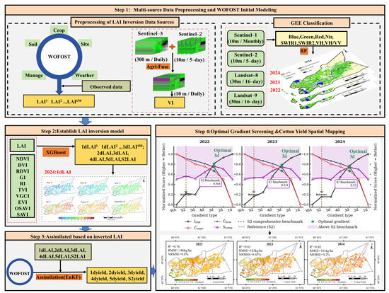
Figure 1. Technical Roadmap.

2. Materials and Methods

2.1. Study Area

Alaer City is located in the northern Tarim Basin of the Xinjiang Uygur Autonomous Region (80°30′–81°58′E, 40°22′–40°57′N). It is a typical oasis agricultural area in an arid region and one of Xinjiang’s important cotton-producing regions (Figure 2). The area has a temperate continental arid climate: annual precipitation is less than 100 mm, annual evaporation is approximately 2200–2600 mm, mean annual temperature is about 10–12 °C, accumulated temperature is roughly 3400–4500 °C, annual sunshine duration exceeds 2800 h, and the frost-free period is about 180–220 days; these climatic conditions are suitable for cotton cultivation (sowing in April, harvesting in October). Soils are mainly sandy loam and loam, with moderate fertility and good permeability; groundwater depth generally exceeds 3 m, and irrigation primarily depends on the Tarim River Basin. However, some fields suffer from severe salinization, which limits cotton growth. Early-maturing, locally adapted cotton varieties are commonly grown, with a planting density of approximately 120,000–150,000 plants·ha⁻¹, combined with plastic mulch and staged irrigation–fertilization management. Nine meteorological stations were deployed in this study (marked as light–blue dots in Figure 2), and the study area was partitioned into nine sub-regions using the Thiessen polygon method. Localized WOFOST calibration was then performed for each sub-region, covering the main cotton-growing areas.

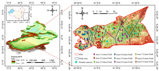
Figure 2. Map of the study area.

2.2. Data

The observational dataset comprises 400 field-site records collected in situ during 2022–2024 (including coordinates and crop type), together with ground observations from 108 cotton fields across nine sub-regions. These field-level samples constitute the ground truth dataset used for the subsequent stages of model development and performance evaluation. At key growth stages (seedling, bud, full flower, and boll opening), a LAI-2200C canopy analyzer (Beijing LiGaoTai Technology Co., Ltd., Beijing, China) was used to measure canopy structural parameters (LAI, mean leaf angle, gap fraction) with 5–10 repeated measurements per plot, and the mean value was recorded. A portable photosynthesis system (LI-6400XT; Beijing LiGaoTai Technology Co., Ltd., Beijing, China) was used to measure leaf transpiration rate, stomatal conductance, photosynthetic rate, and other physiological parameters. At maturity, a five-point sampling method was used: all plants within a 1 m² area of each plot were harvested and oven-dried to determine the total dry weight. Soil samples were collected using a soil corer at depth intervals of 0–20, 20–40, 40–60, 60–80, and 80–100 cm. Samples were dried in an oven at 105 °C to constant weight to calculate their gravimetric moisture content. Yield data were collected and archived via in-field measurements or agricultural sales records. The WOFOST model requires ten categories of input parameters: emergence parameters, phenology (growth stage) parameters, initial conditions, green leaf biomass, assimilation rate, dry-matter partitioning, maintenance respiration, water-use efficiency, root growth parameters, and nitrogen-fertilizer management parameters. Each parameter was obtained by computation or field measurement following the WOFOST manual and temporally processed according to the model’s time-scale requirements.

Multi-source remote sensing data were acquired on the Google Earth Engine (GEE) platform, including Landsat-8/9 OLI, Sentinel-2 MSI, Sentinel-3 OLCI, and Sentinel-1 SAR, for surface feature extraction. Specifically, Landsat-8/9 consisted of on-orbit corrected reflectance products (absolute geolocation error < 12 m), while Sentinel-2 data were used at Level-1C (top-of-atmosphere reflectance). In GEE, a unified projection coordinate system was applied, and data were resampled to a common spatial resolution (10 m in this study) as needed to reduce geometric mismatches. The data preprocessing workflow was as follows. First, optical imagery underwent cloud and cloud shadow masking (utilizing Landsat radiance/brightness temperature/NDSI features, Sentinel-2 QA60 bands, and Sentinel-3 quality indicators). Subsequently, atmospheric correction is performed using the FLAASH algorithm. Sentinel-1 SAR data were processed with orbit parameter correction, thermal noise removal, radiometric calibration, and geometric correction, and monthly median composites were generated to suppress speckle and sporadic noise. Table 1 lists the detailed parameters of the remote sensing data used in this study.

Table 1. Detailed Parameter Information for Remote Sensing Data.

Data Type	Band Numbers	Cloud Cover (%)	Date	Spatial Resolution	Data Usage
Sentinel-1	VV, VH	<10	1 April–1 October, 2022–2024	10 m	Classification
Sentinel-2 MSI	B2, B3, B4, B8, B11, B12	<10	1 April–1 October, 2022–2024	10 m	Classification, Spacetime Fusion
Sentinel-3 OLCI	Oa4, Oa6, Oa8, Oa17	<10	15 May–30 September, 2022–2024	300 m	Spacetime Fusion
Landsat-8 OLI	B2, B3, B4, B6, B7, B8	<10	1 April–1 October, 2022–2024	30 m	Classification
Landsat-9 OLI	B2, B3, B4, B6, B7, B8	<10	1 April–1 October, 2022–2024	30 m	Classification

Meteorological data were obtained from nine stations deployed in the study area, covering daily observations from 1 March to 20 October 2022–2024, including daily maximum/minimum temperature, relative humidity, sunshine duration, wind speed, and daily precipitation. Station observations were assigned to the nine sub-regions using the Thiessen polygon method and used as meteorological inputs for the WOFOST model. Figure A1 (Appendix A) shows the regional variations in temperature, precipitation, and radiation across sub-regions during the full cotton growing period (Day of Year, DOY 92–274).

2.3. Methods

2.3.1. Cotton Planting Area Extraction

To obtain a precise spatial mask for cotton yield estimation, we employed a random forest (RF) classifier on the GEE platform, utilizing a multi-source feature set derived from Landsat-8/9, Sentinel-2, and Sentinel-1 imagery [33]. The analysis covered the main growing season (April to October) for the years 2022–2024. Cloud-masked optical imagery was used to compute key vegetation indices (NDVI, EVI, LSWI, GCVI), which were combined with SAR backscatter features to enhance the separability of cotton from other crops (e.g., maize, wheat). Preliminary tests indicated that Sentinel-2 provided the primary contribution to boundary delineation due to its high spatial resolution (10 m), while the combined Landsat-8/9 time series were crucial for capturing phenological differences to distinguish cotton from maize. The classifier was trained using field survey samples split into 70% for training and 30% for testing. The resulting classification maps achieved an overall accuracy (OA) exceeding 96% and a Kappa coefficient greater than 0.94 across all three years (Figure 3), providing a reliable boundary constraint for the subsequent fusion and assimilation workflows [34].

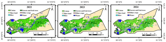
Figure 3. Spatiotemporal distribution of cotton planting areas in the study region for 2022–2024 based on the multi-source RF classification.

2.3.2. Agri-Fuse Algorithm

This study adopted the Agri-Fuse algorithm (https://github.com/GuZhuoning/Agri-Fuse.git, accessed on 5 March 2024) for spatiotemporal fusion of multi-source remote sensing data. The core objective is to improve the spectral fidelity and spatial texture retention of fused images by integrating high-spatial-resolution data (Sentinel-2, 10 m) with high-temporal-resolution data (Sentinel-3, 300 m). This integration overcomes the inherent trade-off between temporal and spatial resolutions, enabling fine-grained monitoring of crop growth dynamics across key phenological periods [19]. The Agri-Fuse algorithm consists of three core steps, incorporating explicit parameter settings and quantitative logic:

(1) Quantitative Classification of Phenological Change Types

First, the predicted-date coarse-resolution image (Sentinel-3) is resampled to the spatial resolution of the base-date high-resolution image (Sentinel-2) using bicubic interpolation. Band-wise difference images are then calculated by subtracting the resampled coarse image from the base-date fine image. This step quantitatively reflects the magnitude of spectral change caused by vegetation phenology:

$$△\mathrm{I}(\mathrm{i},\mathrm{j},\mathrm{k})={\mathrm{F}}_1^{\mathrm{l}}\left(\mathrm{i},\mathrm{j},\mathrm{k}\right)-{\mathrm{C}}_2^{\mathrm{d}\mathrm{o}\mathrm{w}\mathrm{n}\mathrm{s}\mathrm{c}\mathrm{a}\mathrm{l}\mathrm{e}\mathrm{d}}{\mathrm{b}}^{\mathrm{l}}\left(\mathrm{i},\mathrm{j},\mathrm{k}\right)$$

(1)

where $(\mathrm{i},\mathrm{j})$ denotes fine-pixel coordinates and $k$ represents spectral bands.

Subsequently, an unsupervised ISODATA clustering algorithm is applied independently to each band’s difference image. To ensure reproducibility, the key parameters were set as follows: minimum clusters = 2, maximum clusters = 6, maximum iterations = 50, convergence threshold < 1%, and minimum pixels per cluster = 30.

To preserve the spatial structure of farmland parcels, object-based image segmentation was performed using the Segment Only Feature Extraction Workflow (ENVI 5.6). We adopted the Edge algorithm (Scale = 20) for segmentation and Full Lambda Schedule (Scale = 25) for merging. Finally, a 60% majority voting rule was applied: if the dominant change type within a segmented parcel exceeded 60% of the total pixels, all pixels in the parcel were reassigned to this type. This step effectively eliminates “salt-and-pepper” noise and ensures consistent change types within field boundaries.

(2) Class-Based Regression for Spectral Unmixing

Based on the mixed-pixel assumption, a linear regression model was constructed for each change type to characterize the spectral response relationship between base-date and predicted-date images:

$${\mathrm{F}}_2^{\mathrm{l}}(\mathrm{i},\mathrm{j},\mathrm{k})={\mathrm{a}}^{\mathrm{l}}(\mathrm{k})\times {\mathrm{F}}_1^{\mathrm{l}}(\mathrm{i},\mathrm{j},\mathrm{k})+{\mathrm{b}}^{\mathrm{l}}(\mathrm{k})$$

(2)

where ${\mathrm{F}}_2^{\mathrm{l}}$ is the predicted reflectance of a fine pixel for change type $\mathrm{l}$; ${\mathrm{F}}_1^{\mathrm{l}}$ is the base-date reflectance; and ${\mathrm{a}}^{\mathrm{l}}(\mathrm{k})$ and ${\mathrm{b}}^{\mathrm{l}}(\mathrm{k})$ are the regression slope and intercept, respectively. To avoid multicollinearity and enhance stability, we selected the top $\mathrm{p}$ coarse pixels (where $p$ is significantly greater than twice the number of change types) exhibiting the largest spectral change magnitude ($△\mathrm{C}$) to solve the regression coefficients globally for each class.

(3) Residual Compensation via Spatial Filtering

Drawing on the strategy of the Fit-FC algorithm, residual noise in the initial prediction was eliminated by weighting neighboring pixels based on spectral similarity:

$${\hat{\mathrm{F}}}_{2,\mathrm{S}\mathrm{F}}(\mathrm{i},\mathrm{j},\mathrm{k})=\sum _{\mathrm{s}}{\mathrm{W}}_{\mathrm{s}}(\mathrm{k}){\hat{\mathrm{F}}}_2(\mathrm{i},\mathrm{j},\mathrm{k})$$

(3)

where $\mathrm{S}$ denotes the index of spectrally similar neighboring pixels within a 10 × 10 local window. ${\mathrm{W}}_{\mathrm{s}}\left(\mathrm{k}\right)$ is the weight determined by the Euclidean distance and spectral similarity. In this study, only the top 5 most spectrally similar pixels were selected for weighting, ensuring that the final fused value is derived strictly from pixels with consistent phenological traits.

A holistic assessment using Taylor diagrams was adopted [35]. Spectral accuracy was quantified by Root Mean Square Error (RMSE), and spatial structure fidelity was assessed using Local Binary Patterns (LBP). Comparative results indicate that Agri-Fuse outperforms mainstream algorithms (OPDL, RASDF, STARFM, Fit-FC) in both dimensions. Consequently, Agri-Fuse was used to generate time-series datasets with intervals of 1 to 5 days, providing a robust foundation for the subsequent crop model assimilation. To explicitly illustrate the methodological advantages of Agri-Fuse over traditional window-based algorithms in handling mixed pixels, a comparative workflow analysis is presented in Table A1.

2.3.3. WOFOST Model Configuration and Calibration

WOFOST is a process-based dynamic crop growth model that quantifies key physiological processes—such as photosynthesis, respiration, and dry-matter partitioning—by integrating field meteorology, soil properties, and crop parameters. In this study, simulations were implemented using the PCSE 6.0 framework with the WOFOST72_WLP_FD configuration (water-limited production, free drainage), considering the arid ecological setting of the study area. LAI and total weight of storage organs (TWSO) served as the core state variables for evaluating model performance.

To ensure local applicability, we performed a rigorous two-step calibration process using field observations from the 2022–2024 growing seasons. First, phenological parameters (specifically TSUM1 and TSUM2) were adjusted based on observed emergence, flowering, and maturity dates. Second, a global sensitivity analysis (using Sobol’s method) was conducted to identify the key growth parameters affecting yield and biomass accumulation. The analysis revealed that parameters such as the initial total dry weight (TDWI), life span of leaves (SPAN), and maximum leaf CO₂ assimilation rate (AMAXTB) exhibited the highest sensitivity indices [36]. These sensitive parameters were then iteratively optimized to minimize the RMSE between the simulated and observed LAI and TWSO time series. The final calibrated parameter values, compared with the default values derived from the literature [37], are explicitly listed in Table 2.

Table 2. Main parameter values used for calibration of the World Food Studies (WOFOST) mode.

Parameter	Description	Units	Value
Crop initial condition parameters
TDWI	Initial total crop dry weight	kg ha−1	200
LAIEM	Leaf area index at emergence	ha ha−1	0.0045
RGRLAI	Maximum relative rate of increase in LAI	ha ha−1 d−1	0.05
Green area parameters
TBASE	Lower threshold temperature for aging of leaves	°C	10.00
SPAN	Life span of leaves growing at 35 °C	days	64
SLATB00	Specific leaf area at DVS = 0	ha kg−1	0.0016
SLATB058	Specific leaf area at DVS = 0.58	ha kg−1	0.0013
SLATB010	Specific leaf area at DVS = 1.0	ha kg−1	0.0090
SLATB200	Specific leaf area at maturity	ha kg−1	0.0012
Phenological parameters
DLO	Optimum day length for development	h	1.00
DLC	Critical day length	h	0.00
TSUM1	Cumulative temperature from emergence to anthesis	°C	700
TSUM2	Cumulative temperature from anthesis to maturity	°C	1580
Assimilation parameters
AMAXTB00	Maximum leaf CO2 assimilation rate (DVS = 0)	kg ha−1 h−1	50.00
AMAXTB145	Maximum leaf CO2 assimilation rate (DVS = 1.45)	kg ha−1 h−1	62.00
AMAXTB170	Maximum leaf CO2 assimilation rate (DVS = 1.70)	kg ha−1 h−1	65.00
AMAXTB200	Maximum leaf CO2 assimilation rate (DVS =2)	kg ha−1 h−1	58.00
KDIFFTB00	Extinction coefficient for diffuse visible light (DVS = 0)	–
KDIFFTB200	Extinction coefficient for diffuse visible light (DVS = 2)	–
EFFTB0	Light-use efficiency of a single leaf (T = 0 °C)	kg ha−1 h−1 J−1 m2 s−1	0.40
EFFTB40	Light-use efficiency of a single leaf (T = 40 °C)	kg ha−1 h−1 J−1 m2 s−1	0.40
TMPFTB14	Reduction factor of AMAX (T = 14 °C)	–	0.00
TMPFTB26	Reduction factor of AMAX (T = 26 °C)	–	1.00
TMPFTB38	Reduction factor of AMAX (T = 38 °C)	–	1.00
TMPFTB46	Reduction factor of AMAX (T = 45 °C)	–	1.00
Conversion of assimilation into biomass parameters
CVL	Conversion efficiency of assimilates into leaf tissue	kg kg−1	0.72
CVO	Conversion efficiency of assimilates into storage organs	kg kg−1	0.65
CVR	Conversion efficiency of assimilates into root tissue	kg kg−1	0.72
CVS	Conversion efficiency of assimilates into stem tissue	kg kg−1	0.69
Maintenance respiration parameters
Q10	Relative change in respiration rate per 10 °C temperature increase	–	2.00
RML	Relative maintenance respiration rate of leaves	kg CH2O kg−1 d−1	0.0264
RMO	Relative maintenance respiration rate of storage organs	kg CH2O kg−1 d−1	0.0350
RMR	Relative maintenance respiration rate of roots	kg CH2O kg−1 d−1	0.0380
RMS	Relative maintenance respiration rate of stems	kg CH2O kg−1 d−1	0.0060
Partitioning parameters
FRTB00	Fraction of total dry matter to roots at DVS = 0	kg kg−1	0.45
FRTB160	Fraction of total dry matter to roots at DVS = 1.6	kg kg−1	0.00
FRTB200	Fraction of total dry matter to roots at DVS = 2.0	kg kg−1	0.00
FLTB00	Fraction of total dry matter to leaves at DVS = 0	kg kg−1	0.55
FLTB90	Fraction of total dry matter to leaves at DVS = 0.9	kg kg−1	0.53
FLTB103	Fraction of total dry matter to leaves at DVS = 1.03	kg kg−1	0.30
FLTB145	Fraction of total dry matter to leaves at DVS = 1.45	kg kg−1	0.00
FLTB177	Fraction of total dry matter to leaves at DVS = 1.77	kg kg−1	0.00
FLTB200	Fraction of total dry matter to leaves at DVS = 2.0	kg kg−1	0.00
FOTB00	Fraction of total dry matter to storage organs at DVS = 0	kg kg−1	0.00
FOTB90	Fraction of total dry matter to storage organs at DVS = 0.9	kg kg−1	0.00
FOTB103	Fraction of total dry matter to storage organs at DVS = 1.03	kg kg−1	0.23
FOTB145	Fraction of total dry matter to storage organs at DVS = 1.45	kg kg−1	0.96
FOTB177	Fraction of total dry matter to storage organs at DVS = 1.77	kg kg−1	1.00
FOTB200	Fraction of total dry matter to storage organs at DVS = 2.0	kg kg−1	0.00
FSTB00	Fraction of total dry matter to stems at DVS = 0	kg kg−1	0.45
FSTB90	Fraction of total dry matter to stems at DVS = 0.9	kg kg−1	0.47
FSTB103	Fraction of total dry matter to stems at DVS = 103	kg kg−1	0.47
FSTB145	Fraction of total dry matter to stems at DVS = 145	kg kg−1	0.04
FSTB177	Fraction of total dry matter to stems at DVS = 177	kg kg−1	0.00
FSTB200	Fraction of total dry matter to stems at DVS = 2.0	kg kg−1	0.00
Death rate parameters
PERDL	Maximum relative death rate of leaves due to water stress	kg kg−1 d−1	0.03
RDRSTB15001	Relative death rate of stems at DVS = 1.50	kg kg−1 d−1	0.02
RDRDTB200	Relative death rate of stems at DVS = 2.0	kg kg−1 d−1	0.02
Input main soil and site parameters
SMFCF	Soil moisture content at wilting point	cm3 cm−3	0.292
SM0	Soil moisture content of saturated soil	cm3 cm−3	0.42
K0	Hydraulic conductivity of saturated soil	cm d−1	28.97
SOPE	Maximum percolation rate in the root zone	cm d−1	1.32
KSUB	Maximum percolation rate of water into subsoil	cm d−1	2.03
SMLIM	Maximum moisture content in topsoil	cm	0.42
WAV	Initially available water in total root-exploitable soil		50

2.3.4. Assimilation Variable (LAI) Inversion

Based on five sets of time-series fused gradient data and Sentinel-2 raw imagery from April to September 2024, multiple vegetation indices (VIs) were calculated, including NDVI, DVI, RDVI, GI, RI, TVI, VGCI, EVI, OSAVI, and SAVI. These indices reflect vegetation growth status and spectral characteristics from various dimensions. Through Pearson correlation analysis ranking, NDVI, EVI, and SAVI were ultimately identified as the optimal variable combination due to their consistently high correlation with field-measured LAI and resistance to soil background noise. Consequently, these three indices were explicitly selected as the input features for the subsequent inversion models.

Using the selected optimal vegetation indices and their temporal gradients, four models—eXtreme Gradient Boosting (XGBoost), RF, SVM and OLS—were used for LAI inversion [38]. To ensure the scientific rigor of the evaluation and strictly prevent data leakage caused by spatial autocorrelation, a spatially stratified sampling strategy was implemented. The 108 surveyed fields were partitioned into two independent subsets based on the sub-regions described in Section 2.2: a training set comprising 81 fields (9 randomly selected per sub-region) and a validation set comprising the remaining 27 fields (3 per sub-region). As illustrated in Figure 4, the validation samples (represented by red triangles) were spatially disjointed from the training samples (represented by blue circles) across all nine sub-regions. This spatial separation ensures that the validation set provides an unbiased assessment of both LAI inversion and final yield estimation on unseen data. By comparing inversion performances of different models across the temporal gradients, their advantages, disadvantages, and applicability were comprehensively evaluated.

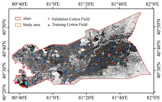
Figure 4. To ensure an unbiased evaluation, 9 fields per sub-region (blue circles) were randomly allocated for model training and 3 fields (red triangles) for validation, guaranteeing spatial disjointness and minimizing autocorrelation effects.

These optimized results served as core observational data. Combined with optimal LAI inversion outcomes from different temporal gradients and original Sentinel-2 imagery, multiple assimilation schemes were constructed. These were contrasted with a non-assimilated scheme (WA) in comparative experiments. Through longitudinal analysis spanning 2022–2024, the assimilation strategies’ effectiveness in enhancing LAI estimation performance was systematically evaluated.

2.3.5. EnKF Assimilation

Based on model calibration, the EnKF algorithm was employed for dynamic assimilation of state variables. As a Bayesian filtering technique, EnKF dynamically updates model states by integrating forecast outputs with observational data, thereby effectively reducing simulation errors [32]. This study determined the LAI observation variance to be 5% by comparing the relative error between field-measured LAI and satellite-derived LAI in cotton fields, setting the ensemble size to 80 members. Let the model state vector be X and the observation vector be y. The core EnKF process comprises two steps:

(1) Prior State Set Generation: Utilize the advancement of set members through model dynamics to obtain the prior state set:

$${\mathrm{x}}_{\mathrm{k}}^{\mathrm{f}\left(\mathrm{i}\right)}=\mathrm{M}({\mathrm{x}}_{\mathrm{k}-1}^{\mathrm{a}\left(\mathrm{i}\right)})+{\mathsf{\epsilon }}_{\mathrm{k}}^{\left(\mathrm{i}\right)},\mathrm{i}=\mathrm{1,2},\dots ,{\mathrm{N}}_{\mathrm{e}}$$

(4)

Here, ${\mathrm{x}}_{\mathrm{k}}^{\mathrm{f}\left(\mathrm{i}\right)}$ denotes the forecast state of the $\mathrm{i}$–th ensemble member, $M$ represents the model operator, ${\mathsf{\epsilon }}_{\mathrm{k}}^{\left(\mathrm{i}\right)}$ is the model noise, ${\mathrm{N}}_{\mathrm{e}}$ is the ensemble size, and $a$ and $\mathrm{f}$ denote the analysis (update) and forecast states, respectively.

(2) Ensemble Member State Update: Update the forecast state ensemble by integrating multi-temporal observations and observation error covariance:

$${\mathrm{x}}_{\mathrm{k}}^{\mathrm{a},\mathrm{i}}={\mathrm{x}}_{\mathrm{k}}^{\mathrm{f},\mathrm{i}}+{\mathrm{K}}_{\mathrm{k}}\left({\mathrm{y}}_{\mathrm{k}}^{\left(\mathrm{i}\right)}-{\mathrm{H}\mathrm{x}}_{\mathrm{k}}^{\mathrm{f},\left(\mathrm{i}\right)}\right)$$

(5)

Here ${\mathrm{y}}_{\mathrm{k}}^{\left(\mathrm{i}\right)}-{\mathrm{H}\mathrm{x}}_{\mathrm{k}}^{\mathrm{f},\left(\mathrm{i}\right)}$ represents the observation with disturbance, where $\mathrm{H}$ is the observation operator and ${\mathrm{H}\mathrm{x}}_{\mathrm{k}}^{\mathrm{f},\left(\mathrm{i}\right)}$ denotes the observation noise. Disturbance is added to preserve variance. The Kalman gain matrix is defined as:

$${\mathrm{K}}_{\mathrm{k}}={\mathrm{P}}_{\mathrm{k}}^{\mathrm{f}}{\mathrm{H}}^{\mathrm{T}}{\left(\mathrm{H}{\mathrm{P}}_{\mathrm{k}}^{\mathrm{f}}{\mathrm{H}}^{\mathrm{T}}+{\mathrm{R}}_{\mathrm{k}}\right)}^{-1}$$

(6)

Here, ${\mathrm{P}}_{\mathrm{k}}^{\mathrm{f}}$ represents the prior state covariance matrix, computed from the ensemble state, while ${\mathrm{R}}_{\mathrm{k}}$ denotes the observation error covariance matrix.

By applying EnKF assimilation, the spatiotemporal distribution of daily LAI was dynamically optimized, enabling high-precision updates to model states. This enhanced the accuracy of cotton growth simulations and provided a foundation for spatiotemporal fusion analysis of multi-source data. Evaluation employed a combined longitudinal comparison and cross-validation approach: longitudinal comparisons assessed the interannual stability of LAI estimates across seven schemes from 2022 to 2024; cross-validation utilized measured LAI data from verification plots to quantify assimilation accuracy improvements using the determination coefficient (R²), RMSE, and Normalized Root Mean Square Error (NRMSE) metrics.

2.3.6. Model Evaluation

To comprehensively validate the proposed framework, model evaluation was conducted across three dimensions: spectral-spatial fidelity, statistical accuracy of yield estimation, and computational efficiency.

First, for spectral and spatial assessment, $\mathrm{R}\mathrm{M}\mathrm{S}\mathrm{E}$ (Equation (9)) served as the criterion for spectral deviations, while the $\mathrm{L}\mathrm{B}\mathrm{P}$ (Equation (7)) was employed as a spatial texture indicator within Taylor diagrams to evaluate structural preservation.

Second, for yield estimation accuracy, standard statistical metrics including the coefficient of determination (${\mathrm{R}}^2$; Equation (8)), $\mathrm{R}\mathrm{M}\mathrm{S}\mathrm{E}$ (Equation (9)), and $\mathrm{N}\mathrm{R}\mathrm{M}\mathrm{S}\mathrm{E}$ (Equation (10)) were selected. To facilitate multi-objective comparison, we aggregated these metrics into a single Statistical Accuracy Index (${\mathrm{I}}_{\mathrm{s}\mathrm{t}\mathrm{a}\mathrm{t}}$) after normalization. Specifically, the three metrics were normalized to a unified scale to eliminate dimensional differences and then averaged to derive a single indicator representing the overall model performance.

Third, to quantify the “Accuracy-Efficiency” trade-off, we introduced two efficiency metrics: Computational Time Cost (${\mathrm{C}}_{\mathrm{t}\mathrm{i}\mathrm{m}\mathrm{e}}$), representing the total CPU processing time for the complete workflow (preprocessing, fusion, and assimilation); and Data Storage Cost (${\mathrm{C}}_{\mathrm{m}\mathrm{e}\mathrm{m}}$), representing the total disk space required.

Finally, a Comprehensive Performance Index (${\mathrm{S}}_{\mathrm{c}\mathrm{o}\mathrm{m}\mathrm{p}}$; Equation (11)) was developed to rank the assimilation schemes (1-day to 5-day intervals). As shown in Equation (11), this index integrates accuracy and efficiency through a weighted linear combination.

$$\begin{array}{c}\hfill \mathrm{L}\mathrm{B}\mathrm{P}=\mathrm{d}\mathrm{e}\mathrm{c}\mathrm{i}\mathrm{m}\mathrm{a}\mathrm{l}({\mathrm{d}}_1,{\mathrm{d}}_2,\cdots ,{\mathrm{d}}_8)\hfill \\ \hfill {\mathrm{d}}_{\mathrm{i}}=\{\begin{array}{ll}1,& \mathrm{i}\mathrm{f} D_i>D_c\\ 0,& \mathrm{o}\mathrm{t}\mathrm{h}\mathrm{e}\mathrm{r}\mathrm{w}\mathrm{i}\mathrm{s}\mathrm{e}\end{array}\hfill \end{array}$$

(7)

$${\mathrm{R}}^2=1-{\displaystyle \frac{\sum _{i=1}^n (y_i-{\tilde{y}}_i{)}^2}{\sum _{i=1}^n (y_i-{\overline{y}}_i{)}^2}}$$

(8)

$$\mathrm{R}\mathrm{M}\mathrm{S}\mathrm{E}=\sqrt{{\displaystyle \frac{\sum _{i=1}^n ({\tilde{y}}_i-y_i{)}^2}{n}}}$$

(9)

$$\mathrm{N}\mathrm{R}\mathrm{M}\mathrm{S}\mathrm{E}={\displaystyle \frac{\sqrt{\frac{\sum _{i=1}^n {\left({\tilde{y}}_i-y_i\right)}^2}{n}}}{{\overline{y}}_i}}$$

(10)

$${\mathrm{S}}_{\mathrm{c}\mathrm{o}\mathrm{m}\mathrm{p}}=\alpha \cdot {\mathrm{I}}_{\mathrm{s}\mathrm{t}\mathrm{a}\mathrm{t}}+\beta \cdot (1-{\widehat{\mathrm{C}}}_{\mathrm{t}\mathrm{i}\mathrm{m}\mathrm{e}})+\gamma \cdot (1-{\widehat{\mathrm{C}}}_{\mathrm{m}\mathrm{e}\mathrm{m}})$$

(11)

where ${\widehat{\mathrm{C}}}_{\mathrm{t}\mathrm{i}\mathrm{m}\mathrm{e}}$ and ${\widehat{\mathrm{C}}}_{\mathrm{m}\mathrm{e}\mathrm{m}}$ denote the min–max normalized values of time and storage costs, respectively. To balance performance requirements with operational constraints, the weights were set to α = 0.5 (accuracy), β = 0.25 (time) and γ = 0.25 (storage). This index enables a quantitative identification of the optimal observation strategy that maximizes accuracy while minimizing resource consumption.

3. Results

3.1. Performance Evaluation of the Agri-Fuse Algorithm

The performance of the Agri-Fuse algorithm [21] was benchmarked against four established methods: OPDL, Fit-FC, RASDF, and STARFM. As illustrated in Figure 5, Agri-Fuse demonstrated superior robustness in preserving spectral fidelity and capturing high-frequency temporal dynamics.

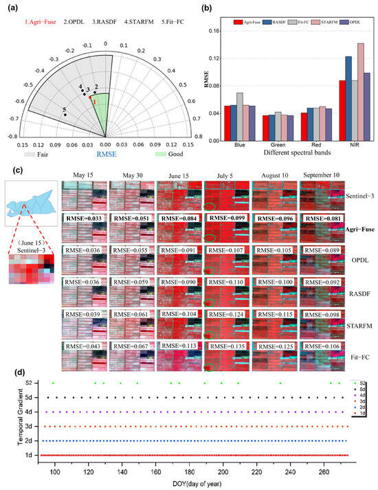
Figure 5. Comprehensive performance assessment of remote sensing data fusion in Aral City (APA), parcel prediction error, and spatiotemporal visualization: (a) The average all-round performance assessment diagrams; (b) Root Mean Square Error (RMSE) of parcel prediction across different spectral bands and methods; (c) Spatiotemporal visualization of remote sensing data fusion results in Aral City. Note: The visualization adopts a false-color composite scheme of NIR-Red-Green bands, where vegetation typically appears in red tones. Left: Study area extent; Right: 2 × 6 layout imagery from 7–12 July (top row: Sentinel-3 raw data; bottom row: left to right—Sentinel-2 raw data and Agricultural Fusion (Agri-Fuse) fusion results). (d) Lower panel: Reflectance time series scatter plot (horizontal axis: time; vertical axis: reflectance).

Quantitatively, Agri-Fuse yielded optimal reconstruction accuracy across varying spectral and spatial resolutions (Figure 5a). With its data points consistently closest to the center line, it achieved the lowest overall RMSE, with all values below 0.10. Furthermore, Agri-Fuse demonstrated advantages across all spectral bands, showing the most significant improvement in the red band, which is responsive to cotton phenological signals. Specifically, it reduced the RMSE by approximately 18% compared to the widely used STARFM algorithm (Figure 5b). The superior performance in this band indicates that Agri-Fuse effectively captures the non-linear spectral variations driven by rapid biomass accumulation. For instance, during the critical peak growth stage (5 July), Agri-Fuse maintained a robust RMSE of 0.099, significantly outperforming STARFM (0.135) and RASDF (0.124), which struggled with complex canopy heterogeneity. This capability effectively mitigates the spectral distortion often observed in linear-based fusion models during dynamic phenological stages.

Visually, the comparison matrix in Figure 5c provides robust evidence of the algorithm’s stability across the full cotton phenological cycle (May to September). While the input Sentinel-3 observations (left Panel) are characterized by coarse pixels that obscure field boundaries, the Agri-Fuse results (Row 2) successfully recover high-frequency spatial details. Attributed to the object-based classification strategy inherent in Agri-Fuse, the fused images preserve clear field boundaries and texture information, exhibiting exceptional consistency with the Sentinel-2 Reference (Row 1). This advantage is most pronounced during the peak growing season (July–August), where cotton fields exhibit diverse and asynchronous phenological changes. As shown in Row 2, Agri-Fuse correctly estimates the reflectance for these heterogeneous parcels. In contrast, traditional methods such as STARFM (Row 6) suffer from evident block artifacts and spectral blurring, arising from their reliance on window-based searching that often fails to capture abrupt changes when adjacent fields undergo different phenological transitions. Furthermore, regarding radiometric consistency, OPDL, Fit-FC, and RASDF exhibited prediction errors for adjacent fields with differing phenological trajectories (highlighted with green circles in the 4th column of Figure 5c), whereas Agri-Fuse accurately retrieved the reflectance for most parcels by effectively handling diverse phenological variations.

These results confirm that the Agri-Fuse algorithm is robust to the temporal distance between the base and predicted dates, effectively overcoming the limitations of single-sensor data. It generates a high-quality, daily spatiotemporal dataset (Figure 5d), providing a reliable foundation for the subsequent LAI inversion and yield estimation.

3.2. Calibration of the WOFOST Model

The temporal dynamics of LAI and TWSO for cotton in the Alaer region (2024) are presented in Figure 6. Quantitative evaluation demonstrated that the calibrated WOFOST model achieved high simulation accuracy. For LAI, the coefficient of determination (R²) reached 0.86 with an NRMSE of 7.2%; for TWSO, the R² was 0.72 with an NRMSE of 11.7%. These metrics confirm that the calibrated model captured the fundamental phenological progression, providing a reliable baseline for the subsequent assimilation strategy.

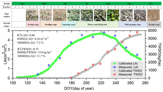
Figure 6. Calibration performance of the WOFOST model for cotton in Aral. The figure illustrates the correspondence between the growth period timeline, field phenological photographs, and the comparison of simulated vs. measured Leaf Area Index (LAI) (green curve/blue scatter) and TWSO (gray curve/red scatter).

3.3. Inversion Accuracy of Assimilation State Variables

Building upon the optimal feature selection (Section 2.3.4), we constructed LAI retrieval models using the fused high-spatiotemporal resolution imagery. A comparative analysis of four machine learning models across five temporal gradients (1-day to 5-day intervals) revealed that the XGBoost model with a 1-day gradient achieved superior performance (Figure 7a). It yielded an R² of 0.97, an RMSE of 0.079, and an NRMSE of 2.8%, demonstrating exceptional capability in capturing dynamic changes and resisting noise compared to the RF, SVM and OLS models. Based on this optimal model, we generated LAI spatial distribution maps for six critical growth stages (Figure 7d), which successfully reproduced the temporal dynamics of cotton: rapid expansion in the seedling stage, peak attainment during flowering, and decline during boll opening. Spatially, lower LAI values were observed along the Tarim River, likely influenced by saline-alkali soil conditions.

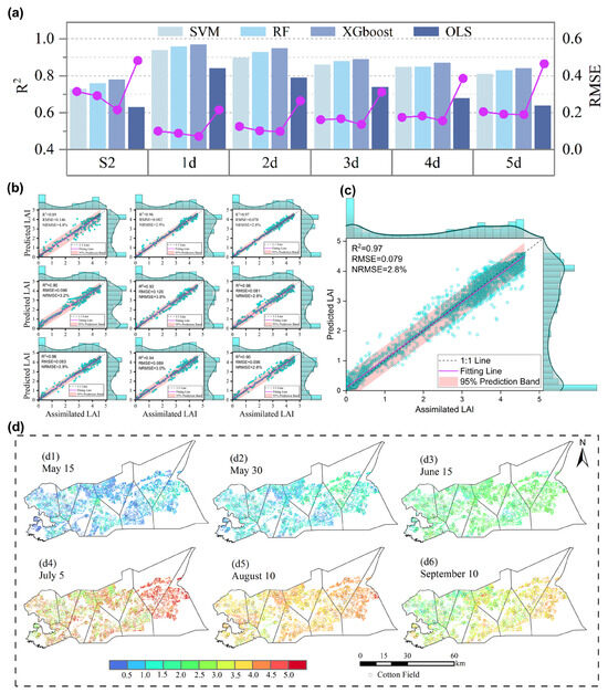
Figure 7. (a) Comparison of LAI inversion accuracy across four models under different temporal gradients in 2024, visually demonstrating the optimal performance of the eXtreme Gradient Boosting (XGBoost) model under a 1-day temporal gradient. Note: The bars represent R² values, and the pink dots represent RMSE values; (b) 2024 leaf area index inversion accuracy validation map (using XGBoost algorithm with 1-day gradient, optimal results at sub-regional scale); (c) 2024 leaf area index Inversion Accuracy Validation Map (using XGBoost algorithm with 1-day gradient, optimal results at county scale); (d) Spatial distribution map of LAI remote sensing inversions during six critical cotton growth stages in Alaer City, 2024. Hollow circles denote LAI values observed at agricultural meteorological stations. Color bars correspond to pixel-level LAI spatial distributions.

To ensure the robustness of the proposed approach, we performed independent validation across both spatial and temporal domains (Figure 7b,c). The validation dataset encompassed observations from all 108 experimental plots spanning the entire 2024 growing season. At the sub-regional scale, R² values consistently exceeded 0.89, indicating stable performance across different zones. At the pan-regional scale, the model achieved an overall R² of 0.97, confirming that the retrieval algorithm maintains high accuracy across heterogeneous land surfaces and dynamic phenological phases.

3.4. Accuracy Assessment of the Coupled EnKF Assimilation Scheme

To evaluate the efficacy of the EnKF strategy, we assimilated the retrieved high-spatiotemporal LAI into the WOFOST model and analyzed the simulation trajectories across two distinct growing seasons, 2023 (Figure 8a) and 2024 (Figure 8b). In both years, the assimilation process significantly corrected the simulated LAI trajectories, effectively pulling the open-loop simulations towards the observed values despite inter-annual climate variability. Specifically for the 2024 growing season, quantitative validation demonstrated substantial accuracy improvements. Compared to the open-loop simulation, the EnKF strategy reduced the divergence between the simulated and observed values. Across all nine sub-regions, the average R² improved from 0.86 to 0.89, the RMSE decreased from 0.26 to 0.22 m²/m², and the NRMSE dropped from 7.2% to 5.8% (Table 3). Region 1 exhibited the most pronounced improvement (NRMSE reduced by 4.1%). These results demonstrate that integrating remote sensing observations via EnKF effectively mitigates model errors caused by initial condition uncertainties, providing a highly accurate physiological foundation for biomass accumulation and yield formation.

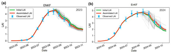
Figure 8. The 2023–2024 LAI assimilation process under the Ensemble Kalman Filter (EnKF) assimilation strategy: (a) 2023 LAI assimilation results; (b) 2024 LAI assimilation results. Blue denotes observed values, green indicates the unassimilated curve, red represents the assimilated curve, and gray lines represent the 79 non-optimal solution curves of the ensemble simulation.

Table 3. Model Performance for LAI Across Nine Cotton Sub-Regions in 2024.

Assimilation Strategy	Without Assimilation			Assimilation LAI
Assimilated Regions	R2	RMSE (m2·m−2)	NRMSE (%)	R2	RMSE (cm3·cm−3)	NRMSE (%)
Region 1	0.75	0.37	12.3	0.83	0.29	8.2
Region 2	0.74	0.38	13.8	0.79	0.32	9.8
Region 3	0.81	0.31	9.6	0.86	0.26	7.1
Region 4	0.78	0.34	11.0	0.84	0.29	8.1
Region 5	0.77	0.35	11.2	0.81	0.30	9.2
Region 6	0.81	0.31	9.9	0.83	0.29	8.9
Region 7	0.85	0.27	7.8	0.87	0.26	6.9
Region 8	0.82	0.29	9.7	0.85	0.27	7.8
Region 9	0.84	0.28	8.9	0.87	0.27	6.5
All cotton fields	0.86	0.26	7.2	0.89	0.22	5.8

Based on the assimilated LAI trajectories, the WOFOST model simulated the biomass accumulation and final yield. The simulated TWSO dynamics effectively reproduced the phenological characteristics of cotton: a gradual increase from the flowering stage, a marked rise during grain filling, and stabilization at maturity (Figure 9a). The EnKF assimilation effectively corrected model biases caused by meteorological fluctuations during the critical flowering and boll-setting stage, aligning the biomass accumulation process more closely with the actual growth rhythm.

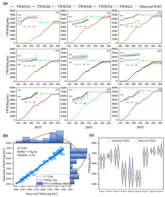
Figure 9. Dynamic Simulation of Cotton TWSO and Accuracy Validation of 2024 Yield Forecast: (a) TWSO simulation covers nine Thiessen polygon sub-regions (Time: late April to late September; Unit: kg/ha). (a1–a9) corresponding to the nine sub-regions respectively. Six curves represent 1d, 2d, 3d, 4d, 5d, and S2 (Sentinel-2) gradients, illustrating cumulative yield dynamics and inter-gradient variations; (b) Scatter plot of 1d gradient simulation values against 108 field-measured yields (unit: kg/ha), including fitted curves and metrics (R², RMSE, NRMSE). Note: Red lines denote marginal lines reflecting data distribution; blue circles represent scatter plot data points; blue bars denote histograms reflecting data distribution; (c) Violin plots of yields across nine sub-regions. Note: Dots represent individual yield data points; short lines denote median values of each sub-region.

Quantitative validation of the yield estimation for 2024 (Figure 9b) indicated that the 1-day temporal resolution scheme performed best, achieving an R² of 0.86, an RMSE of 171 kg/ha, and an NRMSE of 8.2%. This represents a substantial improvement over the non-assimilation scheme (RMSE = 514 kg/ha, see Section 3.2) and the non-fusion (S2 only) scheme (RMSE = 460 kg/ha). The yield distribution analysis across nine sub-regions (Figure 9c) further confirmed that the proposed scheme effectively adapts to underlying surface heterogeneity, such as variations in soil texture and irrigation, maintaining stable estimation accuracy in both high-yield and marginal areas.

3.5. Regional Cotton Yield Estimation and Robustness Analysis

To further verify the system’s temporal robustness and operational applicability, we extended the evaluation to the 2022–2024 period (Table 4). The multi-year analysis consistently showed that increasing the assimilation frequency enhances estimation accuracy; however, this comes with a critical trade-off regarding computational costs (time and storage). While the 1-day scheme yielded the highest accuracy, it requires substantial computational resources, limiting its scalability. As detailed in Table 5 and Figure 10a, a comprehensive evaluation identified the 3-day interval scheme as the optimal configuration for operational applications. It maintained high accuracy (3-year average R² = 0.83, RMSE = 181 kg/ha) while reducing the data processing time and storage volume by approximately 66.5% compared to the daily scheme, effectively balancing algorithmic precision with computational efficiency.

Table 4. Model Comparison of Cotton Yield and Accuracy Across Estimation Schemes, 2022–2024.

Year	2022			2023			2024
Assimilation Strategy	R2	RMSE (kg ha−1)	NRMSE (%)	R2	RMSE (kg ha−1)	NRMSE (%)	R2	RMSE (kg ha−1)	NRMSE (%)
1d-XGboost	0.79	174	8.8	0.85	165	8.4	0.86	171	8.2
2d-XGboost	0.78	180	9.3	0.84	172	9.1	0.85	174	8.9
3d-XGboost	0.77	186	9.8	0.82	183	9.5	0.83	181	9.2
4d-XGboost	0.74	424	10.3	0.79	329	9.6	0.80	304	9.3
5d-XGboost	0.71	457	11.3	0.75	447	10.2	0.76	447	10.3
S2-XGboost	0.73	480	11.4	0.75	466	11.1	0.75	460	10.4
WA	0.69	534	11.8	0.70	526	12.0	0.72	514	11.7

Table 5. Comparison of 3-year average accuracy (R², RMSE, NRMSE) and computational costs (Time, Storage) across different assimilation time intervals.

Assimilation Strategy	R2	RMSE (kg/ha)	NRMSE (%)	Time (h)	Storage (GB)
1d-XGboost	0.83	170	8.5	212.50	251.60
2d-XGboost	0.82	175	9.1	106.25	125.80
3d-XGboost	0.80	183	9.5	71.25	84.34
4d-XGboost	0.78	352	9.7	53.13	63.64
5d-XGboost	0.74	450	10.6	42.50	50.32
S2-XGboost	0.74	467	11.0	18.75	22.20
WA	0.70	525	11.8	2.50	2.96

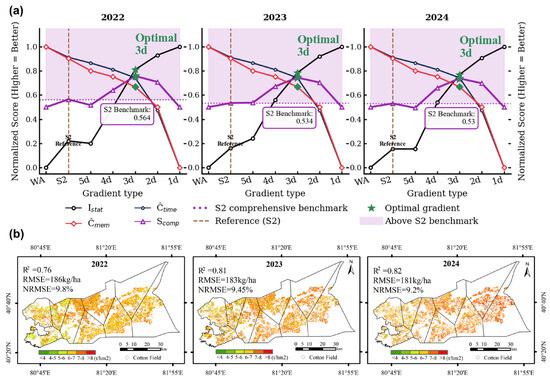
Figure 10. (a) The 2022–2024 comprehensive performance comparison chart. The black line represents the accuracy normalized index, the red line denotes the storage normalized index, the blue line indicates the computational speed normalized index, and the purple line shows the composite index (0–1). The dashed line serves as the S2 gradient comprehensive performance reference line; (b) Spatial distribution and interannual variation of cotton yield in Alaer City, 2022–2024. Color gradient indicates yield levels (unit: kg/ha), with hollow dots denoting yields observed at agricultural meteorological stations.

Deploying this optimized system, we mapped the spatiotemporal trends of cotton yield in Alaer City from 2022 to 2024 (Figure 10b). The results revealed a sustained upward trend in regional yield, with an average annual growth rate of 4.33%. Spatially, high-yield zones have expanded annually, showing strong alignment with the implementation of local agricultural management policies, particularly those promoting water–fertilizer integration and soil amelioration.

4. Discussion

4.1. Accuracy and Robustness of the Assimilation Framework

This study establishes a systematic framework for precision yield estimation in arid oases, effectively addressing the critical “spatiotemporal contradiction” and “data-mechanism disconnect”. The primary contribution lies in the quantitative validation of the “Classification–Fusion–Assimilation” workflow. Foundational to this system, the RF + L9 classification scheme achieved an overall accuracy of 96.05%, providing precise spatial boundary constraints that prevented non-crop noise from propagating into the yield models. Building on this spatial accuracy, our results demonstrate that coupling high-frequency satellite observations with mechanistic models significantly mitigates uncertainties caused by landscape fragmentation and meteorological variability [39]. Specifically, the open-loop WOFOST model, driven solely by meteorological data, suffered from substantial errors (RMSE = 514 kg/ha, NRMSE = 11.7%) due to its inability to account for local stressors like soil salinity. In contrast, the integration of XGBoost-inverted LAI (R² = 0.97) via the EnKF strategy corrected phenological drifts during the critical flowering and boll-setting stages. Crucially, even though this approach updates the state variable (LAI) rather than internal physiological parameters, it effectively re-initializes the biomass accumulation trajectory, drastically reducing the RMSE to 171 kg/ha and NRMSE to 8.2%. This 3.5% reduction in estimation error confirms that constraining mechanistic models with robust satellite observations is not merely an enhancement but a necessity for regional monitoring in data-scarce arid environments [27,40].

4.2. Overcoming the “Blurring Effect” Through Landscape-Adaptive Fusion

Spectral distortion caused by mixed pixels remains a persistent challenge in monitoring fragmented arid agriculture [29]. Standard fusion algorithms, such as Spatial and Temporal Adaptive Reflectance Fusion Model (STARFM), often fail to preserve sharp field boundaries due to linear blending assumptions, leading to significant errors in heterogeneous landscapes. This study quantitatively demonstrates the superiority of the Agri-Fuse algorithm in overcoming this “blurring effect”. By dynamically separating phenological changes from land cover variations, Agri-Fuse achieved a spectral RMSE of only 0.041, significantly outperforming traditional linear models. Notably, in the red band—which is critical for capturing cotton canopy dynamics—Agri-Fuse reduced the prediction error by 18% compared to the widely used STARFM algorithm (Figure 5b). This structural and spectral preservation is vital; it ensures that the foundational reflectance data fed into the subsequent LAI inversion models remain uncontaminated by signals from adjacent shelterbelts or bare soil, thereby preventing the propagation of errors into the final yield estimation [21,34].

4.3. Defining the “Efficiency-Accuracy” Engineering Standard

Beyond theoretical accuracy, this research addresses the operational trade-off between observation frequency and computational cost. The prevailing trend in remote sensing assimilation prioritizes maximum temporal resolution (e.g., daily fusion) [31]. However, our analysis revealed that the “3-day interval strategy” offers the optimal engineering standard for county-level applications. The rationale for this finding is twofold. Agronomically, critical phenological transitions in cotton, such as flowering and boll–setting, typically span several days; thus, a 3-day observation frequency captures these cumulative physiological shifts without missing essential inflection points. While the daily assimilation scheme (1-day) achieved the lowest error (RMSE = 171 kg/ha), the 3-day strategy maintained comparable accuracy (RMSE = 181 kg/ha), resulting in a marginal yield difference of only 10 kg/ha (Table 5). Meteorologically, in arid regions where cloud cover is less frequent than in the tropics, the 3-day strategy offers a robust buffer against data gaps. Crucially, this slight tradeoff was offset for a significant operational advantage: a reduction in computational time and storage by approximately 66.5% (Figure 10a). These findings challenge the “higher is better” assumption, suggesting that a 3-day observation window captures essential phenological inflection points while maximizing system efficiency [28,33].

4.4. Benchmarking, Limitations, and Future Prospects

The yield estimation accuracy achieved in this study (RMSE as low as 171 kg/ha with daily fusion, and 181 kg/ha with the optimal 3-day strategy) significantly outperformed the results reported in both [41] (751 kg/ha) and [42] (999 kg/ha) for similar arid contexts. Furthermore, the estimated annual yield growth of 4.33% (2022–2024) aligns closely with local records of water–fertilizer integration efficacy, validating the model’s agronomic sensitivity.

Despite these successes, limitations remain regarding both the assimilation mechanism and the temporal strategy. First, regarding the model mechanism, the current EnKF framework focuses exclusively on state updating (LAI). It does not explicitly update the posterior distributions of key physiological parameters, such as the maximum CO₂ assimilation rate (AMAXTB) or specific leaf area (SLATB). As highlighted by recent assessments in the Tarim River Basin [20] and global drought studies [43], yield errors in arid regions often stem from incorrect internal parameterization of stress responses rather than just biomass initialization. While our approach successfully rectifies the biomass accumulation trajectory, it may not fundamentally correct the model’s internal physiology under unseen stress conditions, such as varying aerosol loads that alter radiation use efficiency [9].

Second, the conclusion that the 3-day fusion strategy offers an optimal balance is subject to specific boundary conditions. While sufficient for monitoring gradual biomass accumulation in typical years, this frequency may be inadequate for detecting rapid agronomic anomalies. Critical yield-affecting events, such as sudden boll shedding or pest outbreaks, can escalate within 24–48 h, necessitating higher-frequency monitoring for early intervention. Furthermore, from a meteorological perspective, the cost–benefit analysis may shift in years with extreme atmospheric instability. In scenarios with prolonged cloud or dust cover (common in arid springs), the gap-filling value of daily fusion—leveraging the high revisit frequency of Sentinel-3—would increase significantly compared to the 3-day scheme. Therefore, the “3-day optimal” standard should be viewed as a baseline for resource-constrained applications under typical climatic regimes, rather than a universal rule for all stress scenarios [44].

Future iterations should address these dual limitations by: (1) incorporating dual-estimation of states and parameters to enhance mechanistic resilience; and (2) integrating additional high-temporal indicators (e.g., canopy temperature) to capture rapid stress signals that LAI updates might miss.

5. Conclusions

By synergizing the Agri-Fuse algorithm, machine learning classifiers, and the EnKF-assimilated WOFOST model, we constructed a “classification–fusion–assimilation” framework to resolve spatiotemporal inconsistencies in arid oasis agriculture monitoring. This scalable pipeline effectively bridges the gap between data-driven retrieval and process-based crop mechanisms.

Our results demonstrate that the framework significantly enhances regional monitoring capabilities. The enhanced random forest classifier maintained over 96% accuracy in identifying fragmented plots, while the Agri-Fuse algorithm preserved spectral fidelity superior to traditional linear models. Furthermore, we verified that the coupling of XGBoost-inverted LAI with the EnKF-assimilated WOFOST model exhibited robust performance, substantially correcting simulation biases caused by meteorological uncertainties and reducing the yield estimation errors to as low as 171 kg/ha. Crucially, we identified the 3-day Sentinel-2 fusion strategy as the optimal engineering balance: it maintained comparable high accuracy (RMSE difference of only 10 kg/ha) while reducing computational overhead by 66.5% compared to daily schemes. This finding challenges the “higher frequency is better” assumption, offering a robust standard for resource-constrained applications.

Future work will address current limitations regarding the sole reliance on LAI, which may delay the detection of abiotic stresses like soil salinity. We propose incorporating multidimensional state variables (e.g., canopy temperature, soil moisture) and developing dual-estimation methods to enhance resilience against extreme atmospheric instability (e.g., dust storms), thereby strengthening operational robustness in complex arid environments.

References

- Qin, A.Z.; Aluko, O.O.; Liu, Z.X.; Yang, J.C.; Hu, M.K.; Guan, L.P.; Sun, X.W. Improved cotton yield: Can we achieve this goal by regulating the coordination of source and sink? Front. Plant Sci. 2023, 14, 1136636. [Google Scholar] [CrossRef] [PubMed]
- Anees, S.A.; Mehmood, K.; Khan, W.R.; Sajjad, M.; Alahmadi, T.A.; Alharbi, S.A.; Luo, M. Integration of machine learning and remote sensing for above ground biomass estimation through Landsat-9 and field data in temperate forests of the Himalayan region. Ecol. Inform. 2024, 82, 102732. [Google Scholar] [CrossRef]
- Ma, Y.; Zhang, Z.; Kang, Y.; Özdoğan, M. Corn yield prediction and uncertainty analysis based on remotely sensed variables using a Bayesian neural network approach. Remote Sens. Environ. 2021, 259, 112408. [Google Scholar] [CrossRef]
- Zhang, J.; Yang, G.; Kang, J.; Wu, D.; Li, Z.; Chen, W.; Gao, M.; Yang, Y.; Tang, A.; Meng, Y.; et al. Estimation of winter wheat yield by assimilating MODIS LAI and VIC optimized soil moisture into the WOFOST model. Eur. J. Agron. 2025, 164, 127497. [Google Scholar] [CrossRef]
- Reddy, C.S.; Jha, C.S.; Diwakar, P.G.; Dadhwal, V.K. Nationwide classification of forest types of India using remote sensing and GIS. Environ. Monit. Assess. 2015, 187, 777. [Google Scholar] [CrossRef]
- Huang, J.; Tian, L.; Liang, S.; Ma, H.; Becker-Reshef, I.; Huang, Y.; Su, W.; Zhang, X.; Zhu, D.; Wu, W. Improving winter wheat yield estimation by assimilation of the leaf area index from Landsat TM and MODIS data into the WOFOST model. Agric. For. Meteorol. 2015, 204, 106–121. [Google Scholar] [CrossRef]
- Zhou, Y.; Li, F.; Xin, Q.; Li, Y.; Lin, Z. Historical variability of cotton yield and response to climate and agronomic management in Xinjiang, China. Sci. Total Environ. 2024, 912, 169327. [Google Scholar] [CrossRef]
- Torbick, N.; Chowdhury, D.; Salas, W.; Qi, J. Monitoring Rice Agriculture across Myanmar Using Time Series Sentinel-1 Assisted by Landsat-8 and PALSAR-2. Remote Sens. 2017, 9, 119. [Google Scholar] [CrossRef]
- Liu, Y.; Wang, L.; Chen, X.; Niu, Z.; Zhang, M.; Sun, J.; Zhao, J. Quantifying the effects of aerosols and cloud radiative effect on rice growth and yield. Agric. For. Meteorol. 2025, 364, 110453. [Google Scholar] [CrossRef]
- Chen, Y.; Lu, D.; Moran, E.; Batistella, M.; Dutra, L.V.; Sanches, I.D.A.; da Silva, R.F.B.; Huang, J.; Luiz, A.J.B.; de Oliveira, M.A.F. Mapping croplands, cropping patterns, and crop types using MODIS time-series data. Int. J. Appl. Earth Obs. Geoinf. 2018, 69, 133–147. [Google Scholar] [CrossRef]
- Li, J.; Roy, D. A Global Analysis of Sentinel-2A, Sentinel-2B and Landsat-8 Data Revisit Intervals and Implications for Terrestrial Monitoring. Remote Sens. 2017, 9, 902. [Google Scholar] [CrossRef]
- Tang, Y.; Wang, Q.; Tong, X.; Atkinson, P.M. Integrating spatio-temporal-spectral information for downscaling Sentinel-3 OLCI images. ISPRS J. Photogramm. Remote Sens. 2021, 180, 130–150. [Google Scholar] [CrossRef]
- Zhu, X.; Cai, F.; Tian, J.; Williams, T. Spatiotemporal Fusion of Multisource Remote Sensing Data: Literature Survey, Taxonomy, Principles, Applications, and Future Directions. Remote Sens. 2018, 10, 527. [Google Scholar] [CrossRef]
- Zhu, X.; Helmer, E.H.; Gao, F.; Liu, D.; Chen, J.; Lefsky, M.A. A flexible spatiotemporal method for fusing satellite images with different resolutions. Remote Sens. Environ. 2016, 172, 165–177. [Google Scholar] [CrossRef]
- Wang, Q.; Atkinson, P.M. Spatio-temporal fusion for daily Sentinel-2 images. Remote Sens. Environ. 2018, 204, 31–42. [Google Scholar] [CrossRef]
- Gao, F.; Anderson, M.C.; Zhang, X.; Yang, Z.; Alfieri, J.G.; Kustas, W.P.; Mueller, R.; Johnson, D.M.; Prueger, J.H. Toward mapping crop progress at field scales through fusion of Landsat and MODIS imagery. Remote Sens. Environ. 2017, 188, 9–25. [Google Scholar] [CrossRef]
- Zhong, L.; Hawkins, T.; Biging, G.; Gong, P. A phenology-based approach to map crop types in the San Joaquin Valley, California. Int. J. Remote Sens. 2011, 32, 7777–7804. [Google Scholar] [CrossRef]
- Clauss, K.; Yan, H.; Kuenzer, C. Mapping Paddy Rice in China in 2002, 2005, 2010 and 2014 with MODIS Time Series. Remote Sens. 2016, 8, 434. [Google Scholar] [CrossRef]
- Gu, Z.; Chen, J.; Chen, Y.; Qiu, Y.; Zhu, X.; Chen, X. Agri-Fuse: A novel spatiotemporal fusion method designed for agricultural scenarios with diverse phenological changes. Remote Sens. Environ. 2023, 299, 113874. [Google Scholar] [CrossRef]
- Yue, S.; Wang, L.; Cao, Q.; Sun, J. Assessment of Future Cotton Production in the Tarim River Basin under Climate Model Projections and Water Management. J. Earth Sci. 2025, 36, 1780–1792. [Google Scholar] [CrossRef]
- Doraiswamy, P.C.; Hatfield, J.L.; Jackson, T.J.; Akhmedov, B.; Prueger, J.; Stern, A. Crop condition and yield simulations using Landsat and MODIS. Remote Sens. Environ. 2004, 92, 548–559. [Google Scholar] [CrossRef]
- Dumont, B.; Basso, B.; Leemans, V.; Bodson, B.; Destain, J.P.; Destain, M.F. A comparison of within-season yield prediction algorithms based on crop model behaviour analysis. Agric. For. Meteorol. 2015, 204, 10–21. [Google Scholar] [CrossRef]
- Huang, J.; Sedano, F.; Huang, Y.; Ma, H.; Li, X.; Liang, S.; Tian, L.; Zhang, X.; Fan, J.; Wu, W. Assimilating a synthetic Kalman filter leaf area index series into the WOFOST model to improve regional winter wheat yield estimation. Agric. For. Meteorol. 2016, 216, 188–202. [Google Scholar] [CrossRef]
- Wu, S.; Yang, P.; Chen, Z.; Ren, J.; Li, H.; Sun, L. Estimating winter wheat yield by assimilation of remote sensing data with a four-dimensional variation algorithm considering anisotropic background error and time window. Agric. For. Meteorol. 2021, 301–302, 108345. [Google Scholar] [CrossRef]
- Ines, A.V.M.; Das, N.N.; Hansen, J.W.; Njoku, E.G. Assimilation of remotely sensed soil moisture and vegetation with a crop simulation model for maize yield prediction. Remote Sens. Environ. 2013, 138, 149–164. [Google Scholar] [CrossRef]
- Xu, L.; Liu, H.; Jiang, L.; Zhang, F.; Li, X.; Feng, X.; Huang, J.; Bai, T. WOFOST-N: An improved WOFOST model with nitrogen module for simulation of Korla Fragrant pear tree growth and nitrogen dynamics. Comput. Electron. Agric. 2024, 220, 108860. [Google Scholar] [CrossRef]
- Jiang, L.; Zhang, F.; Chi, J.; Yan, P.; Bu, X.; He, Y.; Bai, T. Evaluation of pear orchard yield and water use efficiency at the field scale by assimilating remotely sensed LAI and SM into the WOFOST model. Comput. Electron. Agric. 2025, 233, 110145. [Google Scholar] [CrossRef]
- Li, Q.; Gao, M.; Duan, S.; Yang, G.; Li, Z.-L. Integrating remote sensing assimilation and SCE-UA to construct a grid-by-grid spatialized crop model can dramatically improve winter wheat yield estimate accuracy. Comput. Electron. Agric. 2024, 227, 109594. [Google Scholar] [CrossRef]
- Chakhar, A.; Ortega-Terol, D.; Hernández-López, D.; Ballesteros, R.; Ortega, J.F.; Moreno, M.A. Assessing the Accuracy of Multiple Classification Algorithms for Crop Classification Using Landsat-8 and Sentinel-2 Data. Remote Sens. 2020, 12, 1735. [Google Scholar] [CrossRef]
- Yuan, Q.; Shen, H.; Li, T.; Li, Z.; Li, S.; Jiang, Y.; Xu, H.; Tan, W.; Yang, Q.; Wang, J.; et al. Deep learning in environmental remote sensing: Achievements and challenges. Remote Sens. Environ. 2020, 241, 111716. [Google Scholar] [CrossRef]
- Xu, W.; Chen, P.; Zhan, Y.; Chen, S.; Zhang, L.; Lan, Y. Cotton yield estimation model based on machine learning using time series UAV remote sensing data. Int. J. Appl. Earth Obs. Geoinf. 2021, 104, 102511. [Google Scholar] [CrossRef]
- Huang, J.; Gómez-Dans, J.L.; Huang, H.; Ma, H.; Wu, Q.; Lewis, P.E.; Liang, S.; Chen, Z.; Xue, J.-H.; Wu, Y.; et al. Assimilation of remote sensing into crop growth models: Current status and perspectives. Agric. For. Meteorol. 2019, 276–277, 107609. [Google Scholar] [CrossRef]
- Zhang, X.; Wu, B.; Ponce-Campos, G.E.; Zhang, M.; Chang, S.; Tian, F. Mapping up-to-Date Paddy Rice Extent at 10 M Resolution in China through the Integration of Optical and Synthetic Aperture Radar Images. Remote Sens. 2018, 10, 1200. [Google Scholar] [CrossRef]
- Fei, H.; Fan, Z.; Wang, C.; Zhang, N.; Wang, T.; Chen, R.; Bai, T. Cotton Classification Method at the County Scale Based on Multi-Features and Random Forest Feature Selection Algorithm and Classifier. Remote Sens. 2022, 14, 829. [Google Scholar] [CrossRef]
- Zhu, X.; Zhan, W.; Zhou, J.; Chen, X.; Liang, Z.; Xu, S.; Chen, J. A novel framework to assess all-round performances of spatiotemporal fusion models. Remote Sens. Environ. 2022, 274, 113002. [Google Scholar] [CrossRef]
- Berghuijs, H.N.C.; Silva, J.V.; Reidsma, P.; de Wit, A.J.W. Expanding the WOFOST crop model to explore options for sustainable nitrogen management: A study for winter wheat in the Netherlands. Eur. J. Agron. 2024, 154, 127099. [Google Scholar] [CrossRef]
- Wang, D.; Wang, C.; Xu, L.; Bai, T.; Yang, G. Simulating Growth and Evaluating the Regional Adaptability of Cotton Fields with Non-Film Mulching in Xinjiang. Agriculture 2022, 12, 895. [Google Scholar] [CrossRef]
- Zheng, Z.; Yuan, J.; Yao, W.; Kwan, P.; Yao, H.; Liu, Q.; Guo, L. Fusion of UAV-Acquired Visible Images and Multispectral Data by Applying Machine-Learning Methods in Crop Classification. Agronomy 2024, 14, 2670. [Google Scholar] [CrossRef]
- Wang, H.; Dai, Y.; Yao, Q.; Ma, L.; Zhang, Z.; Lv, X. Multi-task learning model driven by climate and remote sensing data collaboration for mid-season cotton yield prediction. Field Crops Res. 2025, 333, 110070. [Google Scholar] [CrossRef]
- Guo, Y.H.; Hao, F.H.; Zhang, X.; He, Y.H.; Fu, Y.H. Improving maize yield estimation by assimilating UAV-based LAI into WOFOST model. Field Crops Res. 2024, 315, 109477. [Google Scholar] [CrossRef]
- Xing-peng, W.; Fu-chang, J.; Hong-bo, W.; Hui, C.A.O.; Ying-pan, Y.; Yang, G.A.O. Irrigation Scheduling Optimization of Drip-irrigated without Plastic Film Cotton in South Xinjiang Based on Aqua Crop Model. Trans. Chin. Soc. Agric. Mach. 2021, 52, 293–301, 335. [Google Scholar]
- Aziz, M.; Rizvi, S.A.; Sultan, M.; Bazmi, M.S.; Shamshiri, R.R.; Ibrahim, S.M.; Imran, M.A. Simulating Cotton Growth and Productivity Using AquaCrop Model under Deficit Irrigation in a Semi-Arid Climate. Agriculture 2022, 12, 242. [Google Scholar] [CrossRef]
- Chen, X.; Wang, L.; Cao, Q.; Sun, J.; Niu, Z.; Yang, L.; Jiang, W. Response of global agricultural productivity anomalies to drought stress in irrigated and rainfed agriculture. Sci. China Earth Sci. 2024, 67, 3579–3593. [Google Scholar] [CrossRef]
- Ren, S.X.; Chen, H.; Hou, J.; Zhao, P.; Dong, Q.; Feng, H. Based on historical weather data to predict summer field-scale maize yield: Assimilation of remote sensing data to WOFOST model by ensemble Kalman filter algorithm. Comput. Electron. Agric. 2024, 219, 108822. [Google Scholar] [CrossRef]
Disclaimer/Publisher’s Note: The statements, opinions and data contained in all publications are solely those of the individual author(s) and contributor(s) and not of MDPI and/or the editor(s). MDPI and/or the editor(s) disclaim responsibility for any injury to people or property resulting from any ideas, methods, instructions or products referred to in the content. |
© 2026 by the authors. Licensee MDPI, Basel, Switzerland. This article is an open access article distributed under the terms and conditions of the Creative Commons Attribution (CC BY) license.