Highlights
What are the main findings?
- Vegetation index deviations from the field median yield beneficial predictors for random forest models in agricultural applications.
- The VARI, GCC, GLI, and NGRDI indices contain complementary information for detecting Oulema melanopus damage using RGB imagery.
What are the implications of the main findings?
- The approach contributes to Integrated Pest Management decisions within precision agriculture and aids in reducing pesticide use.
- The presented approach contributes to the development of an operational, automated O. melanopus damage detection method for field application.
Abstract
Cereal leaf beetle (CLB, Oulema melanopus L.) is an important pest that damages cereals. Insecticide use against CLB could be reduced with targeted treatments. Our aims were to develop a methodology to map CLB damage on cereal fields using remote sensing. We investigated the suitability of four vegetation indices (VIs: the Visible Atmospherically Resistance Index (VARI), the Green Chromatic Coordinate (GCC), the Green Leaf Index (GLI), and the Normalized Green–Red Difference Index (NGRDI)) derived from RGB images (drone (UAV) imagery). Study sites were located in different regions of Hungary in 2024. Images were taken at different phenological stages of cereals. Suitability of VIs was analyzed with ANOVA and MANOVA. Machine learning models were developed to classify damaged field sections with random forest (RF) and Light Gradient Boosting Machine (LightGBM) algorithms. Results show that VARI, GCC, GLI, and NGRDI contain complementary features for early detection of CLB damage. Difference in sample points’ VI from field median is advantageous for the LGBM algorithm (F1damaged = 0.64–0.72), while the best RF models were obtained with more features (F1damaged = 0.66). Random test data splits had optimistic results (overall accuracy: RF = 0.63–0.80, LightGBM = 0.63–0.79) compared to spatially controlled test splits (overall accuracy: RF = 0.53–0.70, LightGBM = 0.53–0.62).
1. Introduction
Oulema melanopus (Coleoptera: Chrysomelidae), commonly known as the cereal leaf beetle, is an important pest of cereal crops and maize worldwide [1,2]. CLB is native to Eurasia and North Africa [3] and is widely distributed across Europe, ranging from Spain to Sweden, with occurrences in the United Kingdom and Russia [4]. The geographic range and population density of CLB continue to expand. The pest has been listed as an EPPO A1 quarantine organism in Egypt since 2018 and in Canada since 2019 [5,6].
CLB larvae cause significant damage to cereal crops. It has been reported that a density of one larva per stem can cause yield losses of up to 12.65% [7], which corresponds to approximately 0.91 t ha−1, assuming a standard yield of 7.2 t ha−1. According to a Swiss study, each 10% increase in artificial Oulema spp. damage causes a 1.14% yield loss [8]. Assuming 20% leaf damage in a standard field, the yield loss would be 0.164 t/ha. In Hungary, researchers reported a loss of 0.17 g per spike due to 10% flag leaf defoliation and 0.241 g per spike due to 10% whole-leaf defoliation [9]. In a standard winter wheat crop (assuming 1.5 million plants per hectare, each producing three spikes with an average spike weight of 1.6 g, resulting in a 7.2 t ha–1 yield), the yield loss would be 0.765 t ha–1 by 10% flag leaf defoliation and 1.09 t ha–1 by 10% all-leaf defoliation. In addition to yield loss, a considerable decline was found in milling and baking qualities, with a 30% decrease in protein content and 10% reduction in the Hagberg falling number. Without plant protection measures, the progression of leaf defoliation follows a nearly linear trajectory, reaching 35–40% within a 20-day period [2]. The damage can cause total devastation of crop in the stages of leaf development and tillering [10,11]. Moreover, CLB damage increases the probability of infection from plant diseases and water stress in the damaged plant [8,12]. O. melanopus causes more severe damage under warmer, arid climates with low rainfall; therefore, climate change may further contribute to its spread and impact. Changes in pest pressure and phenology under shifting climatic conditions and the ongoing reduction in available plant protection products increase the need for earlier detection and more targeted interventions [2].
CLB has one generation per year. During winter, adults stay in protected sites in small-grain stubble or field boundaries [7]. After winter, the adults fly to cereal crops or grasslands and begin nutritional maturation. Adults feed by biting completely through the leaf tissue, leaving oblong or rectangular holes or ragged notches that often align with the leaf veins. The margins of the injuries appear uneven and torn, with fragments of leaf tissue present, rather than merely scraped off [9,10,13].
After mating, CLB females lay eggs on the surface of the upper leaves [14]. Eggs are mostly laid alone or in duplets or triplets. The eggs hatch after 6 to 10 days, depending on the temperature. The larvae are covered with a dark, fecal shield to protect them. They have four larval instars. At the same temperature, their development takes 11–16 days [10].
Larvae also feed on plant leaves, preferentially targeting young leaves, where they skeletonize the foliage by consuming the upper epidermis and parenchyma, which reduces the leaf area and affects the efficiency of photosynthesis [1,15]. The damage caused by the larvae and the adults can be distinguished because, while the former peels the epidermis and leaves long and thin lines behind, the adults chew through the leaves [16].
CLB exhibits strong aggregation behavior, resulting in pronounced spatial clustering of damage within cereal fields. Geostatistical analyses consistently reveal significant positive spatial autocorrelation and patchiness for all life stages of the CLB, though adults are most frequently aggregated (up to 80% of sampling events), followed by larvae (57%) and eggs (26%). The spatial range of aggregation (i.e., the size of patches) varies from about 39 to 234 m, with an average of 120 m [17,18,19]. Plant stand characteristics affect aggregation: Higher plant density, greater plant height, and more available leaves promote higher establishment and aggregation of larvae, indicating that plant vigor and stand structure are key drivers of beetle clustering [20,21].
The reduction in yield quantity and quality caused by CLB damage is primarily attributable to the reduction in effective photosynthetic leaf area [22]. The observed decline in Soil–Plant Analysis Development (SPAD) relative to the chlorophyll index (RCI) is a substantial decrease in dependent photosynthetic activity, as a result of the reduction in relative chlorophyll content, ranging from 20% to 50%, due to defoliation [2,16]. The physiological responses of the plants to disease or animal pest stresses can be detected in spectral wavelengths by proximal technologies [23]. In the case of CLB, a hyperspectral field spectroradiometer has been used as a proximal sensing tool. The samples were categorized into four levels of damage. Due to damage, changes in plant reflectance were found: an increase in the visible spectrum (400–700 nm) with a pronounced green peak at 550 nm, and a decrease in the near-infrared region (700–1400 nm) [22], similar to other cereal pest species, such as the Russian wheat aphid (Diuraphis noxia) [24]. These changes are indicative of chlorophyll reduction and mesophyll changes [22]. The analytical approach of hyperspectral proximal sensing combined clustering, principal component analysis (PCA), and two machine learning algorithms: Support vector machines and random forest (RF). A range of input data combinations were investigated using nine vegetation indices (NDVI, GNDVI, MTVI2, NPCI, SIPI, (Chl)Rigreen, PRI, REP, and CCI) and PCA-transformed data. The machine learning algorithms attained accuracies ranging from 83.78% to 94.59% in the classification of leaves according to the damage levels [25].
Although these results are encouraging, proximal sensing technologies have several practical limitations, including limited spatial coverage and high time and labor requirements. A more practical and effective method of pest detection is using remote sensing approaches [26,27].
Remote sensing can be conducted across a variety of platforms; the most widely employed are satellites and UAVs. Since the launch of the freely available Sentinel-2 satellite, research in the field of remote sensing has expanded rapidly. Images from the Sentinel 2 satellite were analyzed for pest monitoring of Delottococcus aberiae damage in Spanish orange orchards [28] and for the white coffee leaf miner (Leucoptera coffeella) [29], and they were also applied in crop pest monitoring, such as for the detection of Aphis gossypii in cotton [30], Loxostege sticticalis damage in sunflower [31], and Helicoverpa armigera in maize [32,33]. However, the use of satellite data for detecting pest damage has certain limitations. Satellite-based remote sensing often lacks sufficient spatial resolution for the early detection of pest damage, while ultra-high-resolution images are costly. Satellites have limited revisit frequency and are strongly affected by weather conditions [34,35,36,37].
UAVs are, therefore, increasingly used in remote sensing applications. Using UAV platforms, much higher spatial resolution can be achieved than with satellite-based systems, making them suitable for areas with heterogeneous or sparse vegetation cover [38]. UAVs can carry a wide range of sensors, including RGB, multispectral, and hyperspectral cameras. Among these, RGB cameras are increasingly applied for pest detection, as they are easily accessible (cost, logistics, and availability) [39,40,41,42,43] and, therefore, represent a practical baseline for scalable monitoring. For example, UAV-RGB imagery has been successfully used to develop damage recognition models for Jacobson’s spanworm (Erannis jacobsoni) in forests [34], burning grape leafhopper (Jacobiasca lybica) in grapevine [44], and late blight on potato (caused by Phytophthora infestans) [45]. RGB imagery remains substantially more accessible (cost, logistics, and availability).
Remote sensing is frequently combined with machine learning (ML) algorithms. RGB imagery can further improve pest damage or disease detection accuracy when combined with ML algorithms [46]. For instance, in forestry, UAV-RGB imagery and random forest classification were used to detect parasitic plant mistletoe (Viscum album), achieving an overall accuracy up to 87% in distinguishing infected from non-infected trees [47]. RGB images were used in pine wilt disease detection using a range of ML models, including support vector machines (SVM), random forest (RF), and artificial neural networks (ANN), which reached accuracies of up to 99% [48]. In horticulture, the RF algorithm was used to identify tomato fungal diseases (Alternaria alternata, Alternaria solani, Botrytis cinerea, and Fusarium oxysporum) based on RGB images with 65–87% accuracy [49]. In banana orchards, the combination of RetinaNet and a custom classifier achieved 90.8–99.4% accuracy for distinguishing multiple diseases [50]. Similarly, in field crops, stripe rust disease severity was estimated using random forest classification with 97.9% accuracy based on RGB images [51]. Deep convolutional neural networks (CNNs), such as ResNeSt50, have been successfully applied for identifying Spodoptera frugiperda infestations in maize, achieving up to 98.8% accuracy [52].
However, besides the observed biological factors the reflectance, and due to that the vegetation indices are affected by various environmental factors. The shadows cast on the vegetation reduce the amount of light that reaches the canopy, resulting in lower reflectance values in the affected pixels. This reduction in reflectance can cause vegetation indices to produce artificially low values [53,54,55].
Despite the fact that the CLB causes significant quantitative and qualitative yield losses in cereals and exhibits strong aggregation behavior, site-specific mapping of CLB damage using remote sensing remains poorly explored. Although RGB cameras are becoming increasingly popular for identifying biotic stressors, especially for detecting pests that cause leaf loss, no method has yet been developed for detecting damage caused by O. melanopus.
The purpose of this study is, therefore, to explore the applicability of the RGB camera to map CLB damage, supporting site-specific pest control in accordance with Integrated Pest Management principles [56].
Although deep learning approaches (such as CNN, RetinaNet, etc.) have achieved very high accuracies in RGB remote sensing-based plant stress detection, they usually require large datasets and substantial computational resources. In the present study, we therefore focused on machine learning methods that are still widely used and easier to implement under field conditions [47,49,51].
Our hypothesis was that defoliation by O. melanopus reduces green fraction and alters the chromaticity in RGB, which should increase VIs such as VARI_dif and GLI_dif in damaged areas when compared to controls within the same field, as the reduction in chlorophyll of cereal plants due to O. melanopus has already been reported [2,16], in addition to the fact that RGB vegetation indices are effective proxies for chlorophyll (or LAI as an indicator of chlorophyll) decline (e.g., in the case of VARI [57], GLI [58], and GCC [59]). Our aim was to detect the within-field location of O. melanopus and its damage within the field, using images captured by UAV-mounted RGB cameras, and classify damaged and non-damaged field sections using various combinations of vegetation indices and machine learning algorithms. Our aim is to help farmers to reduce the quantity of insecticides with smart farming technology.
2. Materials and Methods
2.1. Location and Characteristics of the Study Area
The study was conducted in five agricultural fields located within the administrative boundaries of the settlements of Lőrinci and Bölcske, Hungary. Two of the sample fields (L1 and L2) were located near the town of Lőrinci (located on the border between the regions of Central Hungary and Northern Hungary; L1: 47.706147°N, 19.675574°E, amsl: 119 m, 16.8 ha; L2: 47.711433°N, 19.674572°E, amsl: 121 m, 45.14 ha) and three (B1, B2, and B3) were in the catchment area of Bölcske village (located on the border between the regions of Central Transdanubia and Southern Transdanubia, Hungary; B1: 46.752681°N, 18.955356°E, amsl: 137 m, 0.75 ha; B2: 46.757925°N, 18.955040°E, amsl: 136 m, 1 ha; and B3: 46.723882°N, 18.951428°E, amsl: 91 m, 2.75 ha, Figure 1). The vegetation adjacent to the fields was woody, such as woody lines and forests (L1, L2, and B1), arable lands (B3), or both (B2). The cultivated crop was winter wheat in fields L1 and L2, and winter barley in fields B1, B2, and B3. These areas were chosen to represent typical winter cereal agricultural land-use patterns in the region and to provide suitable conditions for testing the aerial and field data acquisition methods.
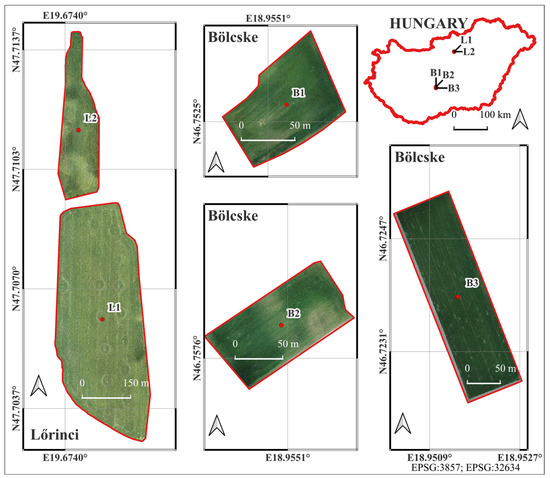
Figure 1.
Study fields damaged by O. melanopus.
2.2. Field Survey
Surveys were conducted on three occasions during the spring–summer growing season. In each survey, the developmental stage of the pest was identified, and plant damage was observed regardless of whether it was caused by adults or larvae. Plant phenology was recorded, and an unmanned aerial vehicle (UAV) flight was conducted for the purpose of imaging the field (Table 1).

Table 1.
The date of field surveys in each sample field, the observed status of Oulema melanopus and the phenology of the crop.
2.2.1. Pest Observation
The first survey was conducted in Lőrinci on 26 March 2024 and in Bölcske on 3 April 2024. In Lőrinci, we established 10 × 10-m sample plots on each field: six of them were damaged by CLBs, and three of them were non-damaged (control). In Bölcske, two damaged and two control sample plots were established in each field. Leaf surface damage was observed from 0.2% to 1.0% in Lőrinci and from 0.5% to 1.0% in Bölcske. Control plots were damaged by 0.1% or less (a maximum of two stripes out of 30 sampled plants, not exceeding 1 mm width). The average number of adult CLB individuals was estimated based on per ten sweep-net sampling. It was 9.5 (ranged 4–23) and 5.8 (ranged 1–14) in Lőrinci and Bölcske, respectively. A total of 350 adult CLB specimens were collected and placed in ventilated vials for species-level identification. It was confirmed that the area was inhabited solely by O. melanopus, with the exception of 1 specimen.
The second survey was conducted in Lőrinci on 26 March 2024 and in Bölcske on 3 April 2024. The developmental stage of the pest larvae was determined. Three plants with pest larvae on their leaves were identified on each sample plot. These plants were photographed with graph paper in the background to determine the size of the larvae.
The third survey was conducted in Lőrinci on 4 June 2024 and in Bölcske on 30 May 2024. It was observed that no pests were present in the field. Ten spikes per sample plot were collected for further analysis.
2.2.2. Image Acquisition
We conducted fifteen (five plots surveyed on three occasions) UAV surveys between 11:30 and 15:15 local time under predominantly clear-sky conditions (cloud cover < 15%) during April–June and applied relative radiometric normalization to mitigate unavoidable seasonal and diurnal variations in solar geometry and illumination.
For the aerial data acquisition, a DJI Matrice 300 RTK (M300 RTK) unmanned aerial vehicle (UAV) equipped with a Zenmuse L1 payload LiDAR (UAV and equipment: Da-Jiang Innovations Science and Technology Co., Ltd., Shenzhen, China) was used (Figure 2) [60,61]. Drone surveys were conducted four times according to Table 1. Although the Zenmuse L1 integrates both LiDAR and RGB sensors, only RGB imagery was used in this study. The Zenmuse L1’s RGB unit features a 1-inch CMOS sensor with an effective resolution of 20 megapixels and a mechanical shutter that supports exposure times ranging from 1/2000 s to 8 s (or up to 1/8000 s electronically).
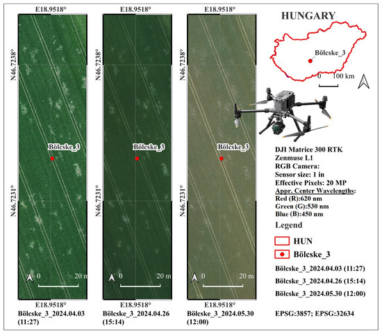
Figure 2.
Conducted drone survey over the “Bölcske 3” field during the tree survey on 3 April 2024 (Survey1), 26 April 2024 (Survey2), and 30 May 2024 (Survey3).
The lens provides a 24 mm equivalent focal length and a variable aperture of f/2.8–f/11, enabling high-quality true-color imagery (photo sizes of 5472 × 3078 (16:9), 4864 × 3648 (4:3), and 5472 × 3648 (3:2)) under various illumination conditions) [60,61]. The ISO range (100–3200 in auto mode; up to 12 800 in manual mode) allows flexible exposure control during field operations. The Zenmuse L1’s RGB sensor uses a conventional Bayer color filter array (CFA) for capturing visible light in the red, green, and blue channels. DJI does not publish exact spectral response curves or filter bandwidths in their official documentation (e.g., user manual or specs sheet). However, based on standard sRGB-compliant digital cameras with similar CMOS sensors, the approximate peak sensitivity (center) wavelengths for the color filters are Red (R): 620 nm, Green (G): 530 nm, and Blue (B): 450 nm [62,63,64]. These are derived from typical Bayer CFA designs used in 1-inch CMOS sensors for photogrammetry and mapping applications [62,63,64].
2.3. Data Processing
2.3.1. Two-Point Relative Radiometric Normalization Using Pseudo-Invariant Features (PIFs)
Radiometric rectification was applied to ensure consistency among UAV-acquired RGB images collected under varying illumination and acquisition conditions [65,66]. Raw digital numbers (DNs) recorded by UAV sensors are strongly influenced by changes in solar geometry, atmospheric conditions, sensor exposure settings, and platform orientation, which can introduce significant bias into multi-temporal analyses. Without normalization, these effects hinder reliable comparison of vegetation indices and may compromise subsequent statistical and machine learning analyses.
To address these issues, a relative radiometric normalization approach was employed to transform all images into a common radiometric domain [65]. This method minimizes radiometric variability unrelated to surface properties, thereby enabling unbiased multi-temporal comparison, vegetation index computation, and damage detection.
Radiometric rectification was performed independently for each spectral band (RGB) using a linear transformation that maps the radiometric characteristics of a subject image to those of a reference image. The transformation for spectral band i was assumed to be linear, such that the rectified pixel value is expressed as follows:
which can be written explicitly as follows:
where denotes the original digital number of the subject image, is the band-specific gain (slope), and is the offset (bias). These parameters were estimated using radiometric control sets.
For each spectral band, two radiometric control sets were defined: a dark control set and a bright control set, representing stable low- and high-reflectance surfaces, respectively. The pseudo-invariant features (PIFs) were selected from stable artificial objects visible in all UAV images [67,68]. The bright control set was defined by the roof surface of our white survey vehicle, whereas the dark control set was derived from the black housing of the UAV, which remained visible in all images throughout the acquisition period. These objects were assumed to exhibit constant reflectance properties over time and were therefore suitable for relative radiometric normalization. The mean DN values of these sets in the subject image are denoted by and , while the corresponding means in the reference image are denoted by and . The linear transformation was constrained to map the dark and bright control sets of the subject image to their counterparts in the reference image:
Substituting the linear form yields the following system of equations:
Solving this system provides closed-form expressions for the transformation parameters. The gain coefficient is given by the following:
and the offset term is given by the following:
This formulation ensures that the dynamic range defined by the dark and bright control sets in the subject image is aligned with that of the reference image.
After estimating the parameters, radiometric rectification was applied to all pixels in the subject image. All computations were performed using floating-point (float32) precision to avoid quantization errors associated with 8-bit imagery. The resulting radiometrically normalized images preserve linear relationships among pixel values while substantially reducing variability caused by acquisition conditions.
Overall, the applied two-point radiometric normalization provides a robust and physically interpretable method for band-wise correction of multi-temporal UAV imagery, ensuring radiometric consistency and improving the reliability of vegetation index-based analyses and machine learning classification.
All image processing was performed using open-source Python 3.13 libraries, including numPy, rasterio, Fiona, Shapely, pandas, and geopandas. From the 8-bit RGB orthomosaic (GeoTIFF format), four vegetation indices were derived, and per-polygon summary statistics were calculated for a set of vector-based sampling units. To ensure reproducibility and efficient memory usage, indices were computed using windowed processing and saved as compressed GeoTIFF files for index computation. The code loads the RGB orthomosaic and processes it in 1024 × 1024-pixel windows to limit memory consumption. For each window, the red, green, and blue bands are read as 32-bit float arrays and scaled to [0, 1] by dividing by 255. An infinitesimal ε = 1 × 10⁻⁶ is added to all denominators to avoid division by zero. The following single-band indices are then computed (according to the equations in Table 2) and saved (Float32, LZW-compressed, and original georeferencing preserved).
Polygon masking and statistics: For each input shapefile (processed recursively from the specified directory), polygon geometries (100 quadrats, each with an area of 1 m2) are read with Fiona and used to mask/crop each index raster (rasterio.mask). Pixels set to NoData = 0 are excluded from the summaries. For every polygon (identified by the grid_id attribute when present), the script computes standard descriptive statistics—count (number of valid pixels), mean, minimum, maximum, and standard deviation—for each index. The pixel count is recorded once (from the GCC layer) to avoid duplication. Results are aggregated into a pandas DataFrame with consistent column naming (VARI_mean, GCC_std, etc.) and exported to a single Excel workbook (.xlsx) per shapefile–raster combination, named <raster>_<shapefile>.xlsx.
2.3.2. Output and File Organization
The workflow creates three output folders: (i) indices (GeoTIFFs of VARI, GCC, GLI, and NDRGI), (ii) statistics (Excel summaries), and (iii) clipped (reserved for intermediate masked rasters; clipping is performed in-memory in the current version). All index rasters inherit spatial reference and geotransform from the source orthomosaic, enabling direct use in GIS or further analysis (Table 2, Figure 3).
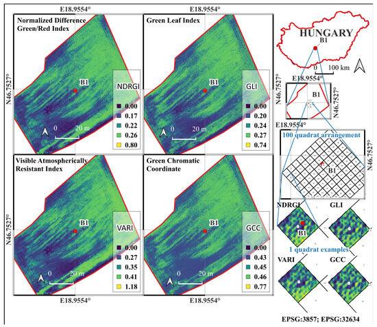
Figure 3.
Spatial distribution of RGB-based vegetation indices—Normalized Difference Green–Red Index (NDRGI), Green Leaf Index (GLI), Visible Atmospherically Resistant Index (VARI), and Green Chromatic Coordinate (GCC)—calculated from UAV-derived orthomosaic imagery over the “Bölcske 1” field site (Hungary) in Survey2 (26 April 2024). The Figure also shows the geographic context, 100-quadrat sampling arrangement, and example quadrats used for index extraction and statistical analysis.
Design considerations: Windowed processing and LZW compression make the pipeline scalable to large orthomosaics; epsilon-stabilized formulas prevent numerical artifacts; and excluding zeros ensures robust statistics when polygons intersect image borders or gaps. The entire workflow is scriptable and portable, facilitating multi-date surveys and consistent, repeatable processing across sites [39,69,70,71,72,73,74,75,76,77].
2.3.3. Selection and Calculation of Vegetation Indices
High-resolution RGB orthomosaics acquired from UAV platforms, such as those produced by the DJI Matrice 300 RTK equipped with a Zenmuse L1 payload, constitute a valuable [42,78], cost-effective resource that facilitates the monitoring of crop conditions and vegetation dynamics, particularly when multispectral data acquisition is constrained by cost or logistical factors [42,78,79,80]. Despite the absence of near-infrared information, several RGB-based indices have been shown to correlate with vegetation parameters such as biomass, canopy cover, chlorophyll concentration, and leaf area index (LAI) [81,82]. Among these indices, the Normalized Green–Red Difference Index (NGRDI), Visible Atmospherically Resistant Index (VARI), Green Leaf Index (GLI), and Green Chromatic Coordinate (GCC) are among the most frequently used RGB-based indices in agricultural remote sensing.
All these four indices are designed for the estimation of the relative greenness of vegetation fraction, which is directly connected to the chlorophyll content of the leaves. The O. melanopus causes significant chlorophyll loss of the leaves, with up to a 40–50% reduction (as measured by the SPAD index) in wheat over a 20-day period [2], and therefore, these indices are potential indicators of chlorophyll loss due to cereal leaf beetle damage.
Although all these indices measure green reflectance, there are differences in their sensitivity to the reflectance in the green band and robustness to different environmental factors such as atmospheric effects.
Table 2.
Equation of vegetation indices calculated in this study.
Table 2.
Equation of vegetation indices calculated in this study.
| Vegetation Indices | Formula A | Ref. |
|---|---|---|
| Visible Atmospherically Resistant Index (VARI) | (G − R)/(G + R − B) | [70] |
| Green Chromatic Coordinate (GCC) | G/(R + G + B) | [83] |
| Green Leaf Index (GLI) | (2G − R − B)/(2G + R + B) | [84] |
| Normalized Green–Red Difference Index (NGRDI) | (G − R)/(G + R) | [70] |
A: Here, R, G, and B denote the red, green, and blue reflectance proxies from the orthomosaic.
Normalized Green–Red Difference Index (NGRDI)
The NGRDI (Table 2) exploits the strong contrast between chlorophyll absorption in the red band and higher reflectance in the green band, making it suitable for assessing vegetation’s vigor, particularly in heterogeneous canopies [70]. Several studies have demonstrated the robustness of NGRDI in vegetation detection and biomass estimation. For instance, Ref. [85] successfully applied NGRDI for weed detection in vineyards, achieving high classification accuracy in differentiating vegetation from soil backgrounds. Similarly, a strong correlation was reported between NGRDI values and aboveground biomass in winter wheat, pea, oat, and mung bean crops, confirming its relevance for growth monitoring and yield estimation [86,87,88]. Although NGRDI’s performance may vary with illumination and spatial resolution, it remains one of the most reliable indices for RGB imagery under controlled acquisition conditions.
Visible Atmospherically Resistant Index (VARI)
VARI was developed to minimize the influence of atmospheric scattering and illumination variability and was successfully applied under variable lighting conditions typical of UAV surveys, as shown in Table 2 [70]. VARI was used for land-use analysis on slopes, where variable atmospheric and lighting conditions were present, and it still obtained consistent vegetation discrimination results [89]. VARI was also applied for rice crop monitoring, demonstrating its sensitivity to vegetation stress [78], and validated its utility in palm tree plantation monitoring [81]. Although VARI may not always outperform indices such as NGRDI in certain vegetation discrimination tasks, it provides reliable results in environments with high illumination variability, which is frequent in UAV operations.
Green Leaf Index (GLI)
GLI (formulated as shown in Table 2) enhances the relative reflectance of the green band and suppresses red and blue components, making it sensitive to the chlorophyll content in a leaf [58]. GLI is more sensitive to the greenness of the vegetation, but less sensitive to blue, and due to that, it is less robust in variable atmospheric conditions [77]. GLI also reduces sensor dependencies by eliminating the sensors’ sensitivity to geometry, scattering effects, and soil color or brightness [84]. This makes it particularly effective for quantifying vegetation cover and assessing canopy density. GLI’s strong accuracy was demonstrated in vegetation recognition using UAV imagery [90] and in land-cover classification using ensemble learning techniques [91]. More recently, smartphone-based GLI could reliably estimate forage quality and dry matter content in steppe rangelands [41]. However, GLI’s performance can vary depending on vegetation type and environmental conditions, requiring calibration to optimize accuracy for specific crops.
Green Chromatic Coordinate (GCC)
The GCC, defined in Table 2, represents the relative proportion of green reflectance within the visible spectrum. It is widely used in canopy phenology and crop growth monitoring [76]. GCC effectively estimated leaf area index (LAI) and dry aboveground biomass (DAGB) in maize [92]. Because GCC normalizes the green reflectance by total visible brightness, it is less sensitive to illumination changes, making it highly suitable for multi-temporal UAV surveys. While the index may require empirical calibration for different crops or lighting conditions, it remains a powerful, simple metric for vegetation greenness.
These models can leverage both redundant and unique features, distributing importance or combining information from weakly correlated indices to achieve superior out-of-sample performance. When computed from radiometrically consistent RGB orthomosaics, as produced by the Zenmuse L1 camera, these indices allow for detailed, reproducible quantification of vegetation conditions at centimeter-level spatial resolution. Their simplicity, computational efficiency, and proven correlation with agronomic parameters make them ideal tools for precision agriculture, crop management, and environmental monitoring, especially when multispectral sensors are unavailable (Figure 3).
2.3.4. Selected VIs in Plant Protection
All selected vegetation indices have previously been applied in crop disease or pest detection studies. All selected vegetation indices were used for crop disease or pest detection. VARI showed a high correlation with the heritability of stink bug resistance in soybean in Brazil [93]. In another study, VARI was used to monitor damage caused by the Moroccan locust (Dociostaurus maroccanus), where reduced green reflectance indicated damaged vegetation [94]. GCC (Green Chromatic Coordinate) was adequate for disease classification with the combination of support vector machines, with above 90% accuracy [95]. In the identification of bacterial leaf blight of rice (Xanthomonas oryzae pv. oryzae), researchers applied GLI (Green Leaf Index) and NGRDI (Normalized Green–Red Difference Index) with the Fuzzy Logic classification technique with 90% accuracy. GLI was more effective in identifying non-paddy areas, whereas NGRDI was proven to be more suitable for detecting diseased paddy regions [96]. GLI (next to RGRI and EGRBDI) had a heightened sensitivity for detecting pest damage or disease on Cinnamomum camphora var. borneol [46]. NGRDI was used for detecting coffee leaf rust (Hemileia vastatrix) and it had 77% accuracy [97].
2.3.5. Labeling Quadrats
Within each study field, each sample plot was subdivided into 1 × 1 m quadrats. For each quadrat, summary statistics of the vegetation indices (mean, median, minimum, maximum, and standard deviation) were calculated. Quadrat- and field-level summaries were then used as inputs for statistical evaluation and modeling.
Each sample plot was labeled with its pest status, indicating whether it was damaged or part of the control group. Each sample plot was visually inspected to identify potential confounding features. In the event of such objects being detected, the quadrat was subsequently labeled. The labels were identified as patchy vegetation, weeds, powerline, and wheel track (Figure 4). The remaining quadrats were labeled according to the pest status of the sample plot. Quadrats labeled as “patchy vegetation” or “weed” were excluded from further analysis due to their low representation.

Figure 4.
Classification of damaged (F12 and F14) and non-damaged control (K9) sample plots in Lőrinci_1 sample field. Wheel track, powerline, patchy vegetation, and weed labels were given to the quadrats that are indicated with the colors in their label. The remaining quadrats in the F12 and F14 sample plots received a damaged label, while the remaining quadrats in K9 sample plot received a control label.
2.4. Statistics, Machine Learning Algorithms, and Model Evaluation
2.4.1. Data Preparation and Analysis of Variance-Based Tests
The statistical analyses were based on the average values of each vegetation index (VI) in 1 × 1 m areas marked as VARI_mean, GCC_mean, GLI_mean, and NDRGI_mean. After assessing data normality, multiway ANOVAs were performed using survey period (factor variable, 3 level), field (factor variable, 5 level), terrain error (factor variable, 3 level: ‘no terrain error’: NE, ‘powerline’: PL, and ‘wheel track’: WT), and pest damage (factor variable, 2 level: ‘damaged’ and ‘control’) as fixed factors. Since the initial analysis revealed an exceptionally large impact of the survey number on VIs, additional multiway ANOVAs were conducted in the second step. These analyses were performed for each survey number separately, including the following three independent variables: fields, terrain error, and pest damage. Since the explanatory effect of the descriptive variables was low according to the multiway ANOVAs run in the first and second steps, the deviation of the values of the vegetation indices from the field median, as well as the field average at each survey time, was calculated using the following formulas:
where VImedif represents the deviation of vegetation index values of each 1 × 1 m plot from the field median (field median-based vegetation index difference values), VImean represents the average vegetation index value of 1 × 1 m plots, and VIfieldmed represents the median vegetation index value on the field level, and the following:
where VIavgdif represents the deviation of vegetation index values of each 1 × 1 m plot from the field average (field average-based vegetation index difference values), VImean represents the average vegetation index value of 1 × 1 m plots, and VIfieldavg represents the average vegetation index value on the field level. The calculated vegetation index difference values (VImedif and VIavgdif) were marked as VARI_medif, GCC_medif, GLI_medif, NDRGI_medif, VARI_avgdif, GCC_avgdif, GLI_avgdif, and NDRGI_avgdif.
VImedif = VImean − VIfieldmed
VIavgdif = VImean − VIfieldavg
The third step of the statistical process was to perform additional multiway ANOVAs for each VImedif and each VIavgdif, considering the effects of terrain error and pest damage. These were conducted separately for each vegetation index and survey time. These multiway ANOVAs were run using a merged two-level factor variable to describe the presence of any type of terrain error in each plot (yes or no), as well as separate two-level factor variables for “powerline” and “wheel track” (yes or no for both), in addition to pest damage. Additionally, the impact of pest damage alone was examined by excluding cases involving any type of terrain error.
In the fourth step, we created a new descriptive variable with six levels. This was derived from a combination of the three terrain error levels (NE, PL, and WT) and the two pest damage levels (‘damaged’ and ‘control’). The dataset was analyzed using one-way ANOVAs for each VImedif and survey period separately. Similar comparisons were planned for each VIavgdif, but this was not presented due to their generally weak explanatory effect.
In the case of ANOVAs performed in any steps, the partial eta-squared (η2p) was also calculated to quantify the percentage of the dependent variable’s variance explained by a single independent variable or interaction. For variables with three or more levels in any ANOVA, a Tukey’s HSD test was used to identify significant differences between levels.
In the case of any MANOVAs or ANOVAs performed in any steps, the available sample size was ensured to meet the requirements of the above statistical tests. The partial eta-squared (η2p) was also calculated to quantify the percentage of variance in the dependent variable explained by a single independent variable or interaction. For variables with three or more levels in any ANOVA, a Tukey’s HSD test was used to identify significant differences between levels.
All statistical analyses were performed at a 95% confidence level using IBM SPSS Statistics 29 software.
2.4.2. Random Forest Algorithm
Random forest (RF) is a non-parametric, ensemble-based machine learning algorithm that combines multiple decision trees trained using bootstrap sampling. It also examines a randomly limited set of features at each split. This approach was shown to reduce variance and the risk of overfitting when compared to individual decision trees [98]. The model also provides feature importance estimates, thereby facilitating feature selection. The RF algorithm has also been successfully applied to the remote sensing detection of other pests [25,34,99,100]. Different sources provide different recommendations regarding the minimum sample size required for the test. While more than 300 samples are generally recommended for environmental modeling, 30 samples often provide a reasonable baseline for many ecological distribution applications, while other references mention 50 samples [101,102].
The present investigation relied on the scikit-learn RandomForestClassifier implementation. The statistical characteristics of all four vegetation indices were integrated into the algorithms. For feature selection, all four vegetation indices were initially retained, and combinations of statistical descriptors were evaluated based on relative feature importance. The hyperparameters were evaluated using 5-fold cross-validation on the training set, where groups were formed by the individual sampling locations. The main hyperparameters were tuned using grid search. Based on the grid search results, we calculated the correlation between cross-validated training performance and each hyperparameter. Model performance was strongly positively correlated with maximum tree depth (r = 0.947), indicating that the performance was primarily driven by tree depth. However, to avoid overfitting, tree complexity constraints were applied, including a maximum tree depth of up to 10 branches. The correlations with the minimum samples per leaf were lower (r = −0.22). A minimum of four training samples should be present within a leaf to reduce the occurrence of “tiny leaves” and facilitate more robust decisions by offering class probabilities that are more stable and less subject to random noise. The possibility of dividing a node was restricted to a minimum of three samples within it. This prevents the further splitting of tiny nodes.
The classes were imbalanced, primarily due to the limited number of wheel track samples. The problem of class imbalance was addressed by implementing the class_weight = “balanced_subsample” option, which assigns weights adjusted to the bootstrap sample in each tree. The decision-making process was refined through the implementation of class-specific post-weighting, whereby the probability output was scaled with class-specific weights. The weights employed in this study were as follows: control = 1.1, damaged = 0.8, and wheel track = 1.0. The slight overweighting of control reduces false “damaged”/“wheel track” alarms, while the slight underweighting of damaged mitigates damage to wheel-track leakage.
2.4.3. Light Gradient Boosting Machine Algorithm
The LightGBM algorithm is a gradient-based boosting decision tree (GBDT) machine learning implementation that was optimized for processing large, high-dimensional datasets [103], but it can also have advantageous properties on small samples. On small samples, histogram-based LightGBM examines fewer thresholds and makes decisions based on aggregated signals, thus learning less from noise while retaining the advantages of GBDT (high accuracy, good weighting). Histogram-based node splitting also ensures its distinctiveness from other decision tree-based algorithms. Due to these properties, we considered its application appropriate in the present research.
The overfitting of the algorithm can be efficiently limited by adjusting parameters. To avoid overfitting, tree complexity reduction and regularization strategies included a maximum of 10 tree depth with a minimum of leaves, and a minimum of 50 child samples. In addition, only 80% of the features are examined in each iteration to enhance the generalization capabilities of the model. To address imbalanced data distribution, class weights were applied after grid search, resulting in damaged: 1.0, control: 1.5, and wheel track: 5.0 weights. Similar to RF, LightGBM was also successfully applied to the remote sensing detection of pests [104].
2.4.4. Validation of Machine Learning Models
Two validation strategies were employed to assess model robustness and spatial generalizability.
The first validation strategy involves the separation of a randomly selected sample quadrat, regardless of its location, as applied in numerous studies [105,106,107,108] REF. A proportion of 30% of the dataset was randomly selected for testing.
The second validation strategy involved a field (section)-level train/test separation. As the inspection was conducted on smaller fields in Bölcske, the data groups comprised individual fields. Conversely, in the case of larger fields in Lőrinci, data were grouped according to predefined field sections where sample plots could be clearly delineated.
To assess the performance of both approaches, a confusion matrix was constructed and used to calculate relevant evaluation metrics, such as overall accuracy (OA), balanced accuracy (BA), and Cohen’s kappa (κ) [109], according to the following equations. The κ was the most important metric:
where the confusion matrix is defined by the following parameters: nij (where j denotes the predicted and i denotes the observed); and N (the total number of observations) for c classes, and pe denotes the expected agreement (by chance).
For each class, precision, recall, and F1-score were calculated to evaluate the most critical failure of the models:
A comparison of the algorithms was conducted through the utilization of geospatially controlled test datasets. The primary decision metrics that were employed are as follows:
- Cohen’s κ.
- Overall accuracy (tree-class evaluation).
It is evident that Cohen’s kappa demonstrates greater resilience in scenarios characterized by class imbalance. However, we prioritized overall accuracy over balanced accuracy, given that the control and damaged classes are balanced. Despite the underrepresentation of the wheel-track class, its significance is comparatively low, thereby reducing its importance for the algorithm in accurately identifying it. In selecting the algorithm, the following three factors were given full consideration: firstly, the results of all three surveys; secondly, the metrics were first ranked and then averaged; and thirdly, the decision was based on direction and stability (variance between surveys).
The workflow of data acquisition and processing, together with the survey timeline, is summarized in Figure 5.

Figure 5.
Data acquisition and processing workflow (Hall et al., 1991 [65]).
Figure 5.
Data acquisition and processing workflow (Hall et al., 1991 [65]).

3. Results
3.1. The Impact of Environmental Factors and Pest Damage on Vegetation Indices
3.1.1. The Impact of Descriptive Variables on the Average Vegetation Index Values
The time of the survey (reflecting the different phenology of the vegetation) had the greatest impact on the VI values. Comparative analysis of environmental and biological factors revealed that all descriptive variables had a significant effect on vegetation indices (VIs). Among the descriptive variables, the time of recording had the greatest impact (η2p: 0.72–0.77). As time progressed, a significant decrease in the values of VIs was observed. The explanatory effect of the fields (η2p) varied between 0.14 and 0.21. The VI values measured in the fields belonging to the two locations did not differ from each other, but the order of values was the same for all VIs. In the case of terrain error, the order of values associated with the levels was found to be inconsistent across all indices examined. However, the discrepancy between NE and PL was only significant for each VI. The effect of the pest damage was significant for all VIs, but this variable explained only 3% of the total variance. The VIs measured in damaged areas consistently exhibited higher values than those recorded in control areas (Table 3).
Table 3.
The effect of environmental factors and pest damage on vegetation indices throughout the entire survey series.
During the first survey period, all descriptives had a significant effect, with the field having the greatest impact. The explanatory effect of the field increased in the comparison between fields based on the data from the first survey period (η2p: 0.10–0.14, all surveys; 0.14–0.21, survey1). By contrast, terrain error (η2p: 0.06–0.07) and pest damage (η2p: 0.03–0.04) had a much greater explanatory effect when the data from the first date were analyzed separately rather than as part of a combined analysis. When analyzing the levels of terrain error, the PL differed significantly from the NE and WT in terms of all VIs. However, the latter two could only be distinguished based on the GLI_mean (Table 4).
Table 4.
The effect of environmental factors and pest damage on vegetation indices at the first survey.
During the second survey period, the effect of the descriptive variables remained significant for each VI. However, these variables explained a smaller proportion of the variance compared to the first period (η2p: 0.05–0.12, field; 0.01–0.04, terrain error; 0.03–0.04, pest damage). Although the field had the greatest explanatory power, no significant differences were found between the B3 and B1, and B3 and B2 fields, in terms of VARI_mean, nor between the B1 and B3, and L2 and B2, fields in terms of NDRGI_mean. Analysis of terrain errors revealed that there was no difference between PL and WT for each VI. However, a significant difference was found between NE and PL for two VIs. Although the multiway ANOVA indicated a significant difference between terrain error levels in VARI_mean and NDRGI_mean, the Tukey HSD test showed no difference between them (Table 5).
Table 5.
The effect of environmental factors and pest damage on vegetation indices at the second survey.
By the third survey, differences among fields became particularly pronounced. This variable explained the largest proportion of variance in vegetation indices (η2p: 0.70–0.74). The explanatory effect of terrain error showed moderate variability (η2p: 0.05–0.09). The difference between NE and PL was significant in all cases, while the difference between NE and WT was significant only in the case of VARI_mean. The partial eta-squared value associated with pest damage was found to be between 0.04 and 0.06 (Table 6).
Table 6.
The effect of environmental factors and pest damage on vegetation indices at the third survey.
3.1.2. The Impact of Terrain Error and Pest Damage on the Vegetation Index Difference Values
For tests based on field median-based vegetation index difference values (VImedif), both terrain error and damage were significant for each VImedif in the first survey period. In the second survey period, several cases were not significant on VARI_medif, and in the third period on VARI_medif, GCC_medif, and NDRGI_medif. For tests based on vegetation index difference values (VImedif), terrain error and damage were significant for all VImedif values during the first survey period. During the second survey period, several explanatory variables in various models were not significant for VARI_medif. The same was true for VARI_medif, GCC_medif, and NDRGI_medif in the third period. The explanatory effect of terrain error remained unchanged compared to the previously applied mean VI values, as the corresponding partial eta-squared value ranged from 0.03 to 0.04. Pest damage explained the variance in VImedif to a slightly greater extent, particularly at the first survey date (η2p: 0.04–0.08), compared to mean VI values. Based on the differentiation of terrain error effects, it can be confirmed that, in most cases, the effect of PL (η2p: 0.02 or below) is significantly lower than that of WT (η2p: 0.03 or below). However, the effect of the WT was not significant in two cases (Survey2 and 3 on VARI_medif). When only data from sampling locations without terrain error is considered in the model, the extent of variance explained by the impact of the pest damage increased at the first (η2p: 0.07–0.16) and third (η2p: 0.01–0.08) survey periods. By contrast, the explanatory effect of pest damage did not exceed 2% at the second survey period, whether the full dataset or the no-terrain-error dataset was used, or any terrain error breakdown method (with terrain errors merged or separated) was applied (Table 7).
Table 7.
The explanatory effect of terrain error and pest damage on field median-based vegetation index difference values resulted by the breakdown method of terrain error cases and by data selection methods.
In general, using VIavgdif resulted in a lower degree of variance explained by the explanatory variables across all VIs and survey periods than when using VImedif.
For instance, in models based on cases with no terrain error, the explanatory effect value (η2p) of pest damage was 0.09 or less for VIavgdif. Furthermore, the effect of pest damage was not significant for GCC_avgdif in the first survey period and for GLI_avgdif in the second (Table 8).
Table 8.
The explanatory effect of pest damage on field average-based vegetation index difference values in the no-terrain-error selection method.
During the first survey, the variable formed by combining pest damage and terrain error showed similar differences across all vegetation indices. The VImedif was significantly higher in NE areas than in WT, in both the damaged and control areas. In contrast, in the comparison between NE and PL, there was no significant difference for any VIs in either the control or the damaged area. The highest values were observed in NE pest-damaged areas for each VI. The lowest values were found in the WT control sample sites for VARI_medif, GLI_medif, and NDRGI_medif, and in the PL control sample sites for GCC_medif (Figure 6).
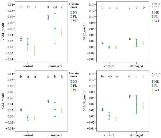
Figure 6.
Deviations in vegetation indices from the field average due to Oulema infection and terrain error at the first survey. NE: no terrain error, PL: powerline, and WT: wheel track. Cases marked with the same letter are not different at a 95% confidence level.
During the second survey period, the value of each VImedif was highest in the WT pest-damaged areas. The terrain error resulted in different patterns for each VImedif. In the control areas, the NE had the highest values. However, comparisons of PL and WT revealed different patterns, with the difference only being significant in the case of GLI_medif and NDRGI_medif. In the pest-damaged areas, no difference was observed between the NE and any terrain error sites (PL or WT) for each VImedif. However, the difference between the PL and WT was significant for GCC_medif and GLI_medif (Figure 7).
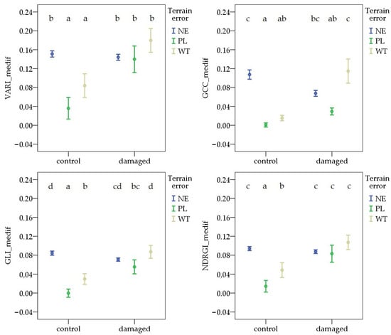
Figure 7.
Deviations in vegetation indices from the field average due to Oulema infection and terrain error at the second survey. NE: no terrain error, PL: powerline, and WT: wheel track. Cases marked with the same letter are not different at a 95% confidence level.
By the third survey, there was a significant difference between the NE and WT for GCC_medif and NDRGI_medif in the control areas, and for VARI_medif, GLI_medif, and NDRGI_medif in the damaged areas. However, the direction of the deviation differed. The values associated with PL were higher than those observed in the NE area for VARI_medif and NDRGI_medif in the control areas. In contrast, the NE values were significantly higher than the PL values for both GCC_medif and GLI_medif in both control and damaged areas (Figure 8).
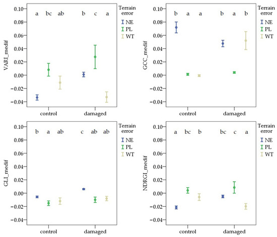
Figure 8.
Deviations in vegetation indices from the field average due to Oulema infection and terrain error at the third survey. NE: no terrain error, PL: powerline, and WT: wheel track. Cases marked with the same letter are not different at a 95% confidence level.
3.2. Classification of Pest-Damaged and Control Quadrats with Machine Learning Algorithms
3.2.1. The Importance of the Different Vegetation Indices as Features of the ML Algorithm
The models were constructed using different statistical characteristics of all vegetation indices (VARI, GLI, GCC, and NDRGI). Results indicate that although relative weights varied among surveys, no vegetation index could be considered negligible, as even the smallest contribution reached 16% (Figure 9).
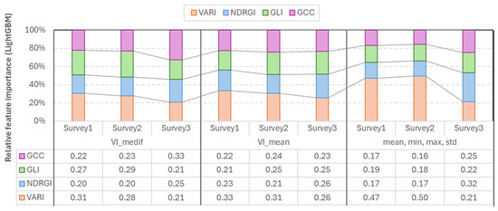
Figure 9.
Relative feature importance of vegetation indices derived from random forest models across the three survey periods.
According to the RF feature importance analysis, each vegetation index contributed across all three surveys, indicating that all retained informative value. During the first two surveys, VARI showed the highest importance (0.28–0.50), while during Survey3, GCC and NDRGI showed increased importance (GCC_medif = 0.33, NDRGI_mean = 0.31, and NDRGI_mean,min,max,std = 0.32).
The LightGBM feature importance analysis confirmed that the most important index varies according to the survey number, and also the higher importance of VARI in the first two surveys. In the case of the mean-based LGBM model, VARI was the strongest (=0.26–0.33) in each survey. In the case of Vmedif-based LGBM models, GLI dominated in the first two surveys (0.35 and 0.28) and GCC (=0.33) in Survey3. The smallest feature importance in this instance was also 0.15, which belonged to GLI in Survey2. In the models where the mean, minimum, maximum, and standard deviation are employed in conjunction, VARI emerges as the leading feature in Surveys 1 and 2, with values of 0.46 and 0.44, respectively. Conversely, GCC and NDRGI demonstrate a corresponding rise in Survey3, reaching 0.3 and 0.29, respectively. However, in the subsequent survey, VARI exhibits a decline. Consequently, the exclusion of any of the indices resulted in a quantifiable decline in performance in at least one survey in LGBM models, and, similar to RF models, LGBM has been shown to effectively handle correlated yet beneficial features; the less significant features are simply less frequently split, rather than being subjected to penalty (Figure 10).
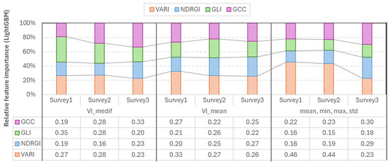
Figure 10.
Relative feature importance of vegetation indices derived from LightGBM models across the three survey periods.
The most important index varies depending on the survey (e.g., time of recording and phenological stage), statistical indicators, and algorithms used; therefore, it is not advisable to rely on a single index. To ensure the robustness of the model, the whole analyzed index portfolio is employed, with this approach being supported by the consistent results of feature importance analysis of the two model families (RF, LGBM).
3.2.2. The Importance of the Different Statistical Parameters of the Vegetation Indices as Features of the ML Algorithm
Overall, the best estimations were obtained using multiple predictors (mean, minimum, maximum, and standard deviation), in both algorithms; however, using VImedif as a single predictor of each VI yielded highly comparable performance, in some cases with higher κ.
The mean of the VIs of the 1 m2 sampling quadrats proved to be a weak estimator. At the first and final surveys, poor estimates were obtained with mean-only features for both RF (accuracy = 0.52, 0.49; Cohen’s κ = 0.25) and LightGBM (accuracy = 0.52, 0.48; κ = 0.27, 0.25), compared to the models based on other predictors. At the second survey, mean-only features resulted in the worst prediction for both RF and LGBM (accuracy = 0.48, 0.51; κ = 0.1, 0.15). For LightGBM, combining multiple statistics yielded the best accuracy for all three surveys (accuracy = 0.68, 0.62, and 0.59); however, κ was lower for the first and third survey (κ = 0.28, 0.34) than the model using the VI-s “medif” parameter as a predictor (κ = 0.30, 0.36). For RF, the best models were based on multiple predictors and reached accuracy = 0.56, 0.70, 0.65, and κ = 0.24, 0.51, 0.43 across the three surveys; however, RF models using VImedif as a predictor reached only slightly lower overall accuracy and Cohen’s κ, meaning a difference of 2% for both predictors (Figure 11).
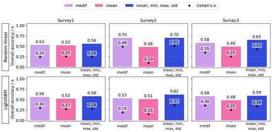
Figure 11.
The overall accuracy (bars) and Cohen’s κ (dots) of random forest and LightGBM algorithms based on different statistical variables of RGB vegetation indices as explanatory variables under a geospatially controlled test set.
3.2.3. Random and Controlled Test Split for Validation
Beyond comparing alternative predictors, how model performance changes was also evaluated when, instead of a conventional random train/test split, the test set was defined as a geospatially delineated field or field-section pretending to be a practical case, when no prior sampling was conducted. Across all three surveys, random splits produced higher overall accuracy and Cohen’s κ than the geospatially controlled test sets. The random data split caused overly optimistic results, regardless of the plant phenology.
For RF, the accuracy gap between random and controlled test sets ranged from 0.07 to 0.2, and κ also differed highly, ranging from 0.1 to 0.36. For LightGBM, the difference between random and spatially controlled testing was also consistently large across all surveys—at least 0.1 in accuracy and 0.14 in κ. Thus, these results indicate that when models involve targets that have spatial attributes, test sets must be defined spatially; otherwise, performance predictions are optimistically biased (Figure 12). Although the models based on VImean showed the same tendency, it was not included in the table as it had previously demonstrated poor performance.
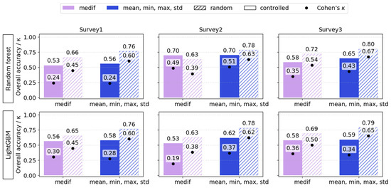
Figure 12.
Overall accuracy (bars) and Cohen’s κ (dots) of VImedif-based and multiple variable (mean, min, and max std)-based random forest and LightGBM under randomly selected training set and geospatially controlled test set across three surveys. Test fields are pure holdouts; random splits are shown to illustrate optimism from spatial leakage.
These findings are consistent with the phenomenon of spatial leakage, whereby random train–test splits permit nearby samples with positively autocorrelated signals to appear in both sets, thereby inflating apparent performance. To mitigate this issue, the test set was defined on a spatial basis, encompassing the entire area that had not been previously sampled. This approach resulted in the production of estimates that were systematically lower and, consequently, more realistic. The pattern was consistent across all three surveys (RF: small gaps in Surveys 1–2, larger in Survey3; LightGBM: consistently large gaps), emphasizing the necessity of evaluating models that exploit spatial structure with spatially explicit splits (e.g., block/leave-location-out cross-validation). It is recommended that spatial validation accuracy and κ be reported as the primary metrics, complemented by uncertainty intervals.
3.2.4. Algorithm Comparison and the Effect of Phenology: Optimal Timing for Detection
The overall performance of RF and LGBM algorithms was extremely similar when a random train–test data split was applied. In contrast, it varied when controlled train–test data splits were used, depending on the survey number (and due to that, on the plant phenology) and also on the feature set.
LightGBM based on mean, minimum, maximum, and standard deviation of the four vegetation indices was identified as the primary model in the first survey, and therefore, during the intensive vegetative growth of cereals. It demonstrated lower κ and accuracy in the second and third surveys compared to the RF models based on the same features. In the second survey, RF VImedif yielded a more competitive κ, and therefore, it was retained as a reference model. The disparities manifested as moderate variations, with typical values of Δκ ranging from 0.01 to 0.29, ΔOA 0.00–0.16, and ΔBA 0.01–0.14. The collective trend across the three surveys demonstrated a pronounced inclination in favor of RF using multiple statistical parameters and LightGBM using VImedif as features, as evidenced in Table 9.
Table 9.
Overall metrics of random forest and LightGBM algorithms on test sets with different feature sets and data split modes.
The overall metrics reveal that the most optimal models were mainly generated at Survey2. This time point corresponded to the termination of the pest’s damaging period (Figure 13).

Figure 13.
The influence of phenology (Survey1—vegetative stage, Survey2—spike emergence, and Survey3—ripening) on the overall accuracy (bars) and Cohen’s κ (dots) of VImedif-based (purple) and multiple variable (mean, min, and max std)-based (blue) random forest and LightGBM under randomly selected test set and a geospatially controlled test set.
From a pragmatic perspective, if the classification of the “damaged” class is the primary objective, the algorithm selection was also evaluated by “damaged” class-level recall and secondarily on precision. Consequently, we prioritized the option that identified a higher proportion of “damaged” class, even if this approach led to a moderate decline in accuracy.
Overall, the damage class mainly has higher precision compared to the other two classes, while control usually has higher recall. In each model, wheel tracks had the least precision, as well as recall (Table 10).
Table 10.
Per class metrics (Precision, Recall, F1 score) of both Random forest and LightGBM models based on VImedif-based and multiple variable (mean, min, and max std)-feature set.
In Survey1, LightGBM demonstrated a higher recall with both feature sets (0.6 and 0.7) compared to random forest (0.66 and 0.68), while RF showed higher precision with multiple feature sets (0.64 vs. 0.59). In Survey2, LightGBM outperformed the other algorithm in terms of damage recall with both feature sets, with 0.87 and 0.56 compared to 0.67 and 0.55 recall of RF. However, RF demonstrated higher damage recognition precision (0.7 and 0.82) compared to LightGBM’s 0.51 and 0.64. In Survey3, the two algorithms were not consistent throughout the feature sets. In accordance with the primary criterion, Survey1 endorses the preference for the LightGBM algorithm with VImedif features, while Survey2–3 support the RF with the multiple feature selection (Table 10).
For both models, changes in recall for the damaged class can be observed from Survey1 to Survey3. The changes in RF were 0.55–0.67, and those with LightGBM were 0.87–0.56, with the advancement of plant growth and phenology, indicating the best recall in Survey2. In parallel, both LightGBM and RF demonstrated a decrease in damage precision by the time of Survey2, indicating an improvement in the number of hits but a decrease in the clarity of the results. Conversely, RF precision showed a moderate increase, from 0.67 to 0.82, with the multiple feature set.
The initial identification of the wheel track class proved challenging (low F1 in Survey1: RF 0.06 and 0.08, and LGBM 0.09 and 0.28). However, both models demonstrated a consistent improvement over time. Nonetheless, the wheel track class demonstrated the poorest performance, particularly in the initial survey.
Both the overall accuracy and kappa values appeared to suggest that the most effective models were developed based on the second survey, and a closer examination of the damage class endorses this conclusion. The enhancement in the overall model can be attributed to the enhanced detection of the wheel track and the stability (RF) or the improvement (LGBM) of the control recall in the models executed prior to harvesting, as well as a slight decrease at the time of spike emergence (Survey2).
Furthermore, confusion matrices were used to assess the severity of critical classification errors. A critical error occurs when damaged areas are incorrectly classified as control. If damaged areas are misclassified as wheel tracks, the resulting error is considered less critical. In such cases, the affected areas would still be treated with pesticides. Similarly, if control is categorized as ‘damaged’, the same course of action will be taken.
From a farming perspective, the most significant issue arises when the model categorizes a value belonging to the damaged class as control, as this diminishes the efficacy of plant protection. An examination of the dates and algorithms from this perspective was also undertaken with confusion matrices.
In the case of Survey1, the VImedif feature set RF algorithm classifies 39.7% of the damaged class as the control class, while in the case of the LightGBM model, this portion is only 37,6% (Figure 14). The RF algorithm classified 95% of the misclassified damaged errors in the control class, while the LightGBM algorithm placed 93%, indicating that almost all of the misclassified damage both algorithms place on the control class, which is the critical error. In the case of multiple feature sets, the RF algorithm misclassifies 33% of the damaged class as the control class, while LightGBM misclassifies only 28% of the damaged class as the control class. The RF algorithm put 95% of the misclassified damaged in the control class, and the LightGBM algorithm put 93% of the misclassified damaged in the control class. It can thus be concluded that, in the intensive vegetation growth phenological stage, when the damage is beginning, the misclassification of both algorithms with both feature sets was the critical error.
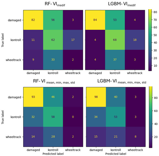
Figure 14.
Confusion matrix of VImedif-based and multiple variable (mean, min, and max std)-based random forest model and LightGBM model under geospatially controlled test set for Survey1.
For Survey2, the RF with the VImedif algorithm misclassifies 24% of the damaged class as the control class, while LightGBM only misclassifies 2%. Out of all its misclassifications of the damaged class, RF placed 72% into the control class, whereas for LightGBM, this figure was 16% (Figure 15). Consequently, most of the RF algorithm’s errors are placed in the control class, which is the critical error, while for LightGBM, it is a very low portion, with a low portion of damage misclassification. This led to only a few critical errors. For the multiple feature set, the RF algorithm misclassifies 35% of the damaged class as the control class, and LightGBM misclassifies 34%. Out of all its misclassifications of the damaged class, RF placed 78% into the control class, while for LightGBM, this was 80.3%. This implies that with multiple feature sets, the two algorithms have a similar number of critical errors.
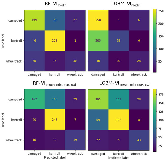
Figure 15.
Confusion matrix of VImediif-based and multiple variable (mean, min, and max std)-based random forest model and LightGBM model under geospatially controlled test set for Survey2.
For Survey3, in the VImedif feature set, the RF algorithm misclassified 15% of the damaged class as the control class, while LightGBM only misclassified 9%. Out of all its misclassifications of the damaged class, RF placed 34% into the control class, and for LightGBM, this figure was 32% (Figure 16). Consequently, a third of both algorithms’ errors are placed in the control class, which is the critical error. For the multiple feature dataset, the RF algorithm misclassifies 31% of the damaged class as the control class, and LightGBM misclassifies 27%. Out of all its misclassifications of the damaged class, RF placed 42% into the control class, while for LightGBM, this was 28%. This implies that RF has a greater tendency to misclassify true damaged instances as control (the critical error) compared to LightGBM.
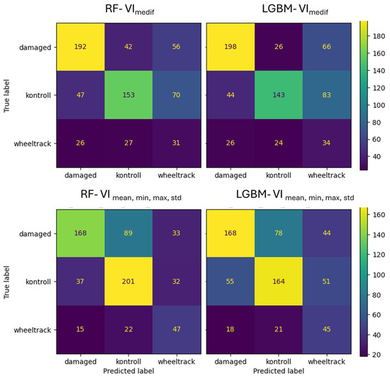
Figure 16.
Confusion matrix of VImediif-based and multiple variable (mean, min, and max std)-based random forest model and LightGBM model under geospatially controlled test set for Survey3.
4. Discussion
Our results indicate that survey timing had the greatest influence on vegetation index values. This finding is consistent with previous studies showing that seasonal variation in plant growth, development, and environmental conditions strongly influences vegetation indices [110]. In our study, we examined the cereal fields from mid-season to the onset of maturation. However, significant differences in VIs may also be caused by the physiological changes that occur during this period, such as defoliation and chlorophyll reduction. Changes in each VI followed a similar trend, with only minor variations [111].
Our study also found that the fields demonstrated a significant impact on VI values. In general, the effect of the location on plant reflectance is significant [112], but these differences were also significant between fields within the same location that were managed using the same agronomic practices (e.g., same crops, cultivars, tillage methods, and sowing times) and experienced similar environmental conditions. This is related to the fact that VIs can be explained by additional human and environmental factors [113,114,115].
Both vegetation cover and visibility can be altered by different types of terrain error [116]. In our study, vegetation indices were reduced by both powerline interference and wheel-track damage. This finding is consistent with the established correlation between vegetation cover and vegetation indices [70].
Although the impact of insect damage on individual vegetation indices was statistically significant, its overall effect size was modest. Although it is important to detect pests early on for effective control, it can be challenging to remotely sense minor infestations in the early stages [117]. Previous studies indicate that the most effective pest detection approaches often rely on more sophisticated deep learning models [118,119].
The confounding effects of survey timing and field location were mitigated by standardizing vegetation index values using field-level medians. Statistical analyses performed in this way revealed that pest damage had a greater explanatory effect than existing terrain errors. However, pest damage alone accounted for only 1–8% of the variation in individual vegetation indices. Powerline interference exhibited lower explanatory power than wheel-track effects. This is related to the extent of the surface area they affect [120]. Additionally, the explanatory effect of pest damage was notably stronger when comparing areas without terrain error, particularly for VARI and NGRDI in the first survey. However, this alone is insufficient to reliably distinguish between infected and uninfected areas.
In conclusion, the field median-based intra-field normalization (VImedif) provides additional information for damage detection. This transformation mitigates global illumination, topography, and other effects and amplifies the “relative to what” type of signal, which is particularly relevant in the damaged vs. control separation. Although this procedure can offset variability caused by field characteristics, further studies should also consider farming factors that may affect vegetation index values, such as crop type [121], phenology [122], soil management [123], and fertility [124]. However, applying field median-based intra-field normalization (VImedif) revealed that the model accounted for a greater proportion of the observed variation, compared to the use of VImean. The partial eta-squared is a useful starting point for a power analysis [125]. Nevertheless, the magnitude did not reach the expected level (for example, the increase in η2p for VARI_medif in the first survey was from 0.04 to 0.07) [126].
The feature importance analysis of the two ML (RF and LightGBM) models showed that the collective inclusion of VARI, NGRDI, GCC, and GLI provides a more comprehensive, resilient, and ultimately more predictive model than any single index could offer alone, leading to stronger, time-robust performance.
Incorporating these vegetation indices into the machine learning algorithms was advantageous because they provide complementary insights, resulting in more reliable predictions over time.
Each of these indices leverages the spectral properties of vegetation within the visible range, where chlorophyll absorbs strongly in the red and reflects strongly in the green. Together, they provided complementary insights into CLB damage. VARI is effective during periods of intense greening at the vegetative phenological phase of plants, while NDRGI becomes more important with a higher portion of soil [85]. Furthermore, these indices exhibit varying resilience to noise and distortion profiles, such as lighting, shadows, and the color of the soil background. VARI is partially atmosphere-resistant [70], GLI is robust to global light fluctuations [84], GCC handles channel contrast effectively [76,90,92], and NDRGI is more sensitive to the green–red portion [70]. This diversity ensures that the algorithm can account for a wide range of environmental conditions and data quality issues. Incorporating these diverse indices into these tree-based machine learning models created a synergistic effect. Therefore, the collective strength of these complementary indices ensures the most robust and accurate predictive capabilities. Similarly to our studies, VIs were combined and incorporated into ML algorithms to predict/detect crop pests or their damage [25,46,100].
In the context of both RF and LGBM, the integrated incorporation of the four selected VImedif yielded highly comparable performance in comparison to models based on averages and combinations of averages with other statistics, across both primary indicators (accuracy, κ). This finding indicates that VImedif optimizes the bias–variance balance when presented with a limited yet informative and complementary set of features.
Consequently, when combining multiple vegetation indices algorithms, it is recommended to consider the use of VIdif, even for other purposes.
The implementation of random test data selection has been demonstrated to yield considerably enhanced test outcomes in comparison to the alternative of spatially controlled and limited testing, which is consistent with the findings of Ramezan et al. [127]. Consequently, within the context of agricultural research, it is imperative to geospatially delimit the area that contains data that is not used for model training, thereby ensuring the development of models that are not excessively optimistic. This discrepancy can be attributed to spatial autocorrelation and background variations (soil, micro-relief, and treatments). In the case of a random split, the test distribution is more closely aligned with the training distribution. Consequently, spatially blocked or grouped validation (e.g., GroupKFold group = table; spatial block CV; and leave-one-field-out) is mandatory in agricultural remote sensing tasks, and practical suitability must be assessed on this basis [128,129,130,131].
In machine learning, this increases the risk that the model partly learns neighborhood similarity (and shared local conditions) rather than true generalizable relationships. If training and test data are spatially close, information leakage can occur, and performance may look artificially high. The optimism of random data splits could be highly derived from the biology of O. melanopus. Because Oulema melanopus shows a strongly aggregated spatial distribution, observations from nearby sampling points (quadrats) tend to be more similar than distant ones. This creates spatial autocorrelation, meaning the data violates the independence assumption.
Aggregation can also leave spatially structured residuals (clusters of over- or underprediction), indicating remaining autocorrelation and underestimated uncertainty.
When examining the CLB damage to winter cereals, the most accurate modeling results were consistently obtained on the second sampling date. This period coincided with the end of larval feeding, making it not optimal from a practical point of view. During this critical phenological phase, the growth rates of the plant and the pest are proportional: the cereal ends its intensive vegetative growth phase, and spikes appear, while the larvae finishes its active feeding period. The rate of plant biomass and chlorophyll loss caused by the pest (‘the plant outgrows the pest’) reached its maximum. Consequently, the impact of pest damage becomes more detectable.
Moreover, CLB larvae primarily feed on the upper leaves; however, as heading begins and progresses, the canopy’s structure and, therefore, reflection characteristics change. The appearance of spikes and the partial shading of the upper leaves modify the reflectance, reducing spectral detectability by UAV.
Studies have identified specific phenological phases that have been shown to be more effective than others when remote sensing was used to assess different characteristics of the fields. The strongest correlations between the canopy reflectance and VIs with regard to yield, dry matter weight, leaf nitrogen, and chlorophyll content were observed during the filling stage [36]. In the context of predicting yield, a combination of different phenological phases has been identified as the most suitable [132]. Conversely, other studies have identified the maximal correlation with yield three months post-sowing [133,134]. Also, a limited period of vegetation was found to be suitable to assess H. armigera damage in maize [32].
Limitations and Outlook
Despite the encouraging results of this study, it is imperative to acknowledge the limitations and disadvantages of the employed interpretation framework. The limiting factors appeared on several interrelated levels, from imaging conditions to data structure to modeling and interpretation conclusions.
The imaging technique holds some limitations, as the spectral signal may vary not only for biological reasons, but also due to the geometry of the imaging and the operation of the sensor. Although the measurements were taken at the same time period of the day (11 a.m. to 3 p.m.), small changes in the solar elevation angle and acquisition geometry may vary, causing edge effects and reflectance shifts [135]. This effect may be confused with biological differences [136]. In connection with illumination, the high vegetation density as a circumstance of our study holds some uncertainties as well, as the plants’ leaf structures shaded the damaged leaves, making noise in the spectral signal, which has been generally reported to have an influence on the vegetation indices [53]. Another important limitation may be the effect of the camera’s automatic settings, e.g., JPEG compression, which can create noise or mask differences [137].
Similarly, limitations associated with the spatial resolution of 1m*1m may have limited the accuracy of the models. At this spatial resolution, a single pixel often contains a mixture of soil, vegetation, and shadow. This produces mixed pixels, leading the model to learn a mixed signal and thereby reducing class separability. In the present study, pixels with sparse vegetation were removed; therefore, the dominant confounding factor is likely to be shadowing associated with the vertical canopy, which was reported to have a significant effect on the reflectance [138]. Therefore, our classification model could be improved with the use of higher-resolution spectral data. However, it would also require a more detailed pest survey of the field to be carried out. Further research on the effect of spatial resolution could be analyzed in terms of the Oulema spp. damage detection problem. Furthermore, an enhancement in the spatial resolution of the estimates for other pests resulted in more accurate models [139,140,141,142,143,144,145,146,147,148], in terms of RGB image analysis, and super-resolution image detection is frequently reported with high accuracy [47,51].
The imbalance of classes had a negative effect on the model, mainly due to the presence of wheel tracks. It is important to note that powerlines were not a significant factor according to ANOVA, thus indicating that they did not represent a separate class and were removed to reduce signal noise. In connection with this, a limitation will emerge in practical use, when powerlines are present in the field, they will require another model to mask them out of the spectral dataset. This also applies to other objects and artifacts appearing on the table.
However, the spectral signal of the wheel track was not negligible. The presence of wheel tracks frequently appears on crop fields in practice, and they are consistently underrepresented compared to the vegetation, as in our study. Therefore, it is a very frequent case in practice that wheel tracks need to be distinguished from damage, despite the accused imbalance of the data. From a model development perspective, it is recommended that further studies increase the sample size of the ‘wheel track’ class in subsequent data collection. This prompts the consideration of two-level models; however, the availability of ‘wheel track’ data for this analysis was limited in the present study. The efficacy of two-level models has also been demonstrated in the context of other pests [149,150,151,152,153,154,155].
A notable disadvantage of the current model is its inability to consider the extent of the damage, which can result in noise arising from varying levels of damage. It is important to note that no high-level damage was observed, and the damage to the leaf surface was minimal. This might result in the algorithm facing a challenging learning environment. It can be hypothesized that data acquisition from fields with a higher level of damage, potentially categorized by damage level, could facilitate more accurate estimation of the models. As indicated by the findings of other studies, the accuracy of models is reduced at low damage levels [118,156].
In addition to the impact of CLB damage, the integrity of images can be compromised by several factors. These include plant diseases (e.g., leaf spots, viruses) and abiotic stresses such as water shortage, heat and frost stress, nutrient deficiency or accumulation, soil salinity, wind and ice damage, and herbicide phytotoxicity. These confounding effects can act as false damage: symptoms can spectrally resemble the pattern caused by CLB, which can push the classification toward false positives. An important limitation is that there was no separate ground truth available for these, and therefore, our results are valid only in the absence of these other types of biotic and abiotic stress symptoms.
Furthermore, factors such as soil heterogeneity, crop phenological status, and cultivation practices (e.g., irrigation, fertilization) have also been demonstrated to influence the spectral signal. During the present study, no visible indications of disease were observed in the fields; however, the impact of abiotic stressors was not examined. Therefore, the results should be considered in the context of this limitation.
Moreover, the data originate from the same year and region, there is a risk of “domain overfit,” and performance may be weaker in other years, under different light conditions (evenings), in other varieties, or in other phenology between studied phenology. Further studies would be beneficial with finer temporal resolution, focusing on the main damage period.
The present study examined the RGB range exclusively, omitting other spectral ranges, as studies reveal that CLB damage causes unambiguous changes in the visible range, especially in the green range [22]. However, it was also clearly evidenced that the structural and pigmentary changes caused by CLB damage are expressed not only in the visible range, but also in the NIR and SWIR bands. More specifically, an increase in reflectance in the visible range (400–700 nm) was typically observed (due to chlorophyll loss), while in NIR/SWIR, changes in cell structure and water content caused characteristic decreases [25]. Therefore, the incorporation of NIR and SWIR bands, using a multispectral camera for the damage classification models, may enhance the accuracy (reducing misclassification due to leaf structural changes).
Regarding further directions for modeling and possible methodologies, they can be incorporated into the working processes of precision agriculture.
For pests that are prone to aggregation, such as Oulema species, a new protocol can be incorporated to avoid autocorrelation by incorporating the geolocation of the data into model development and train–test splits. It is recommended to create smaller blocks with a separate distance between them. Then, the blocks should be grouped into larger blocks according to their spatial location: fields or field sections. Perform the train–test split between these fields of field sections so that the individual field data are not mixed. This is particularly important when developing ML for the detection of pests prone to aggregation in order to reduce the chance of autocorrelation and optimistic models.
Including statistical factors that promote normalization in ML models can help achieve faster processing with low resolution.
In the long term, with a sufficiently reliable model in the future, an automated analysis can be performed based on a field survey to indicate where pests are and are not present. Based on this information, a map for site-specific applications could be created and sent to a precision sprayer. The sprayer would then apply insecticide only where necessary, reducing unnecessary environmental impact and costs in precision agriculture.
5. Conclusions
Based on the results, the combination of VARI, GCC, GLI, and NGRDI constitutes a complementary feature set for the early detection of O. melanopus damage. Using the difference in the sample points’ vegetation index from the field mean (VImedif) is methodologically beneficial, compared to using means only; however, RF and LGBM models reach a higher accuracy with broad feature sets, even in small datasets.
In the context of agricultural remote sensing, machine learning applications require spatially explicit geolocation of test data, as random splits tend to produce overly optimistic performance estimates. Under low damage levels and a 1 × 1 m spatial resolution, random forest and LightGBM models based on RGB-derived vegetation indices (VARI, GCC, GLI, and NGRDI) were insufficient for precision farming applications, as the accuracy and Cohen’s kappa values from spatially controlled validation remained only moderate to high. Consequently, these models require further refinement. Further development should ideally coincide with the mass hatching of CLBs, as it is also the most suitable time from a plant protection perspective.
Supplementary Materials
The following supporting information can be downloaded at: https://www.mdpi.com/article/10.3390/rs18010058/s1.
Author Contributions
Conceptualization, F.E.S.-B. and M.Z.; methodology, F.E.S.-B., M.Z. and G.K.; software, F.E.S.-B., M.Z. and G.K.; validation, F.E.S.-B., M.Z. and G.K.; formal analysis, F.E.S.-B. and M.Z.; investigation, F.E.S.-B., M.Z. and G.K.; resources, F.E.S.-B., M.Z. and G.K.; data curation, F.E.S.-B., M.Z. and G.K.; writing—original draft preparation, F.E.S.-B., M.Z., A.Z.S. and G.K.; writing—review and editing, Z.P. and J.K.; visualization, F.E.S.-B., M.Z. and G.K.; supervision, Z.P. and J.K.; project administration, F.E.S.-B. and M.Z. All authors have read and agreed to the published version of the manuscript.
Funding
The authors received no financial support for the research, authorship, and/or publication of this article.
Data Availability Statement
Our processed data presented in this study are available as Supplementary Materials, along with overall results and per class metrics of all combinations of data split mode, survey number, algorithm.
Acknowledgments
The authors would like to express their gratitude to Gergő Beke for his contribution to the field validation data collection. The authors also thank the expert colleagues from the KITE Innovation Department for their professional support in the identification of the adult moth specimens. We thank Caleb Melenya Ocansey for carefully reviewing the manuscript and for editing and polishing the English to improve clarity, readability, and overall language quality.
Conflicts of Interest
The authors declare no conflicts of interest.
Abbreviations
The following abbreviations are used in this manuscript:
| CLB | Cereal leaf beetle (Oulema melanopus L.) |
| VI | Vegetation index |
| NE | ‘No error’ level of terrain error |
| PL | ‘Powerline’ level of terrain error |
| WT | ‘Wheel track’ level of terrain error |
| VImedif | Field median-based Vegetation index difference value |
| VIavgdif | Field average-based vegetation index difference value |
| VARI | Visible Atmospherically Resistant Index |
| GCC | Green Chromatic Coordinate |
| GLI | Green Leaf Index |
| NGRDI | Normalized Green–Red Difference Index |
| OA | Overall accuracy |
| BA | Balanced accuracy |
| RF | Random forest |
| LightGBM | Light Gradient Boosting Machine |
References
- University, U.S.; Evans, E.W. Cereal Leaf Beetle (Oulema melanopus). In Burleigh Dodds Series in Agricultural Science; Idaho, U., Eigenbrode, A., Tech, U.V., Eds.; Burleigh Dodds Science Publishing: Cambridge, UK, 2023; pp. 3–32. [Google Scholar]
- Keszthelyi, S.; Hoffmann, R.; Lukács, H. Objective Assessment of the Damage Caused by Oulema Melanopus in Winter Wheat with Intensive Cultivation Technology Under Field Conditions. AgriEngineering 2024, 6, 4538–4548. [Google Scholar] [CrossRef]
- Hervet, V.A.D.; Cárcamo, H.A.; Dosdall, L.M.; Miller, T.D.; Kher, S.V. Assessment of Potential Non-Target Effects of Tetrastichus Julis, a Biological Control Agent of the Cereal Leaf Beetle, Oulema melanopus. BioControl 2016, 61, 399–411. [Google Scholar] [CrossRef]
- Oulema melanopus (LEMAME) [World Distribution]| EPPO Global Database. Available online: https://gd.eppo.int/taxon/LEMAME/distribution (accessed on 29 October 2025).
- Regulated Organisms in Canada|EPPO Global Database. Available online: https://gd.eppo.int/country/CA/regulated (accessed on 29 October 2025).
- Regulated Organisms in Egypt|EPPO Global Database. Available online: https://gd.eppo.int/country/EG/regulated (accessed on 29 October 2025).
- Buntin, G.D.; Flanders, K.L.; Slaughter, R.W.; Delamar, Z.D. Damage Loss Assessment and Control of the Cereal Leaf Beetle (Coleoptera: Chrysomelidae) in Winter Wheat. J. Econ. Entomol. 2004, 97, 374–382. [Google Scholar] [CrossRef][Green Version]
- Steinger, T.; Klötzli, F.; Ramseier, H. Experimental Assessment of the Economic Injury Level of the Cereal Leaf Beetle (Coleoptera: Chrysomelidae) in Winter Wheat. J. Econ. Entomol. 2020, 113, 1823–1830. [Google Scholar] [CrossRef]
- Császár, O.; Tóth, F.; Lajos, K. Estimation of the Expected Maximal Defoliation and Yield Loss Caused by Cereal Leaf Beetle (Oulema melanopus L.) Larvae in Winter Wheat (Triticum aestivum L.). Crop Prot. 2021, 145, 105644. [Google Scholar] [CrossRef]
- Kher, S.V.; Dosdall, L.M.; Cárcamo, H.A. Biology, Host Preferences and Fitness of Oulema Melanopus (Coleoptera: Chrysomelidae), a Recent Invasive Pest in Western Canada. Arthropod-Plant Interact. 2016, 10, 365–376. [Google Scholar] [CrossRef]
- Ramsden, M.W.; Kendall, S.L.; Ellis, S.A.; Berry, P.M. A Review of Economic Thresholds for Invertebrate Pests in UK Arable Crops. Crop Prot. 2017, 96, 30–43. [Google Scholar] [CrossRef]
- Cai, R. Herbivorous Insects in Barley Cultivation: Impact and Control Methods. Mol. Entomol. 2024, 15, 69–77. [Google Scholar] [CrossRef]
- Batistič, L.; Vučajnk, F.; Vidrih, M.; Horvat, A.; Košir, I.J.; Šilc, U.; Bohinc, T.; Trdan, S. Evaluating Locally Sourced Inert Dusts as Insecticides against the Cereal Leaf Beetle (Oulema melanopus [L.]; Coleoptera: Chrysomelidae): A Combined Laboratory and Field Study. Cogent Food Agric. 2024, 10, 2415393. [Google Scholar] [CrossRef]
- Kher, S.V.; Dosdall; Carcamo, H. The Cereal Leaf Beetle: Biology, Distribution and Prospects for Control. Prairie Soils Crops J. 2011, 4, 32–41. [Google Scholar]
- Philips, C.R.; Herbert, D.A.; Kuhar, T.P.; Reisig, D.D.; Thomason, W.E.; Malone, S. Fifty Years of Cereal Leaf Beetle in the U.S.: An Update on Its Biology, Management, and Current Research. J. Integr. Pest. Manag. 2011, 2, C1–C5. [Google Scholar] [CrossRef]
- Lukács, H.; Jócsák, I.; Somfalvi-Tóth, K.; Keszthelyi, S. Physiological Responses Manifested by Some Conventional Stress Parameters and Biophoton Emission in Winter Wheat as a Consequence of Cereal Leaf Beetle Infestation. Front. Plant Sci. 2022, 13, 839855. [Google Scholar] [CrossRef]
- Reay-Jones, F.P.F. Spatial Distribution of the Cereal Leaf Beetle (Coleoptera: Chrysomelidae) in Wheat. Environ. Entomol. 2010, 39, 1943–1952. [Google Scholar] [CrossRef] [PubMed]
- Reay-Jones, F.P.F. Spatial Analysis of the Cereal Leaf Beetle (Coleoptera: Chrysomelidae) in Wheat. Environ. Entomol. 2012, 41, 1516–1526. [Google Scholar] [CrossRef][Green Version]
- Reay-Jones, F.P.F. Geostatistical Characterization of Cereal Leaf Beetle (Coleoptera: Chrysomelidae) Distributions in Wheat. Environ. Entomol. 2017, 46, 931–938. [Google Scholar] [CrossRef]
- Kher, S.V.; Dosdall, L.M.; Cárcamo, H.A. Plant Vigor Metrics Determine Spatio-Temporal Distribution Dynamics of Oulema Melanopus (Coleoptera: Chrysomelidae) and Its Larval Parasitoid, Tetrastichus Julis (Hymenoptera: Eulophidae). Environ. Entomol. 2014, 43, 1295–1308. [Google Scholar] [CrossRef] [PubMed]
- Reisig, D.D.; Bacheler, J.S.; Herbert, D.A.; Heiniger, R.; Kuhar, T.; Malone, S.; Philips, C.; Tilley, M.S. Cereal Leaf Beetle (Coleoptera: Chrysomelidae) Regional Dispersion and Relationship With Wheat Stand Denseness. Environ. Entomol. 2017, 46, 425–433. [Google Scholar] [CrossRef] [PubMed]
- Skendžić, S.; Zovko, M.; Lešić, V.; Živković, I.P.; Lemić, D. Detection and Evaluation of Environmental Stress in Winter Wheat Using Remote and Proximal Sensing Methods and Vegetation Indices—A Review. Diversity 2023, 15, 481. [Google Scholar] [CrossRef]
- Wenjiang, H.; Yue, S.; Yingying, D.; Huichun, Y.; Mingquan, W.; Bei, C.; Linyi, L. Progress and Prospects of Crop Diseases and Pests Monitoring by Remote Sensing. Smart Agric. 2019, 1, 1–11. [Google Scholar]
- Mirik, M.; Michels, G.J.; Kassymzhanova-Mirik, S.; Elliott, N.C. Reflectance Characteristics of Russian Wheat Aphid (Hemiptera: Aphididae) Stress and Abundance in Winter Wheat. Comput. Electron. Agric. 2007, 57, 123–134. [Google Scholar] [CrossRef]
- Skendžić, S.; Novak, H.; Zovko, M.; Živković, I.P.; Lešić, V.; Maričević, M.; Lemić, D. Detecting Cereal Leaf Beetle (Oulema Sp.) Damage on Winter Wheat: A Fusion of Proximal Remote Sensing and Advanced Machine Learning; Union of Japanese Societies for Insect Sciences: Kyoto, Japan, 2024. [Google Scholar]
- Ghajar, S.; Tracy, B. Proximal Sensing in Grasslands and Pastures. Agriculture 2021, 11, 740. [Google Scholar] [CrossRef]
- Verma, B.; Porwal, M.; Jha, A.K.; Vyshnavi, R.G.; Rajpoot, A.; Nagar, A.K. Enhancing Precision Agriculture and Environmental Monitoring Using Proximal Remote Sensing. J. Exp. Agric. Int. 2023, 45, 162–176. [Google Scholar] [CrossRef]
- Della Bellver, F.; Franch Gras, B.; Moletto-Lobos, I.; Guerrero Benavent, C.J.; San Bautista Primo, A.; Rubio, C.; Vermote, E.; Saunier, S. Pest Detection in Citrus Orchards Using Sentinel-2: A Case Study on Mealybug (Delottococcus aberiae) in Eastern Spain. Remote Sens. 2024, 16, 4362. [Google Scholar] [CrossRef]
- Vilela, E.F.; Ferreira, W.P.M.; Castro, G.D.M.; de Faria, A.L.R.; de Leite, D.H.; Lima, I.A.; Matos, C.d.S.M.d.; Silva, R.A.; Venzon, M. New Spectral Index and Machine Learning Models for Detecting Coffee Leaf Miner Infestation Using Sentinel-2 Multispectral Imagery. Agriculture 2023, 13, 388. [Google Scholar] [CrossRef]
- Fu, H.; Zhao, H.; Song, R.; Yang, Y.; Li, Z.; Zhang, S. Cotton Aphid Infestation Monitoring Using Sentinel-2 MSI Imagery Coupled with Derivative of Ratio Spectroscopy and Random Forest Algorithm. Front. Plant Sci. 2022, 13, 1029529. [Google Scholar] [CrossRef]
- Kara, S.; Maden, B.; Ercan, B.S.; Sunar, F.; Aysal, T.; Saglam, O. Assessing the Impact of Beet Webworm Moths on Sunflower Fields Using Multitemporal Sentinel-2 Satellite Imagery and Vegetation Indices. Int. Arch. Photogramm. Remote Sens. Spat. Inf. Sci. 2023, 48, 521–527. [Google Scholar] [CrossRef]
- Sári-Barnácz, F.E.; Zalai, M.; Toepfer, S.; Milics, G.; Iványi, D.; Tóthné Kun, M.; Mészáros, J.; Árvai, M.; Kiss, J. Suitability of Satellite Imagery for Surveillance of Maize Ear Damage by Cotton Bollworm (Helicoverpa armigera) Larvae. Remote Sens. 2023, 15, 5602. [Google Scholar] [CrossRef]
- Sári-Barnácz, F.E.; Zalai, M.; Milics, G.; Tóthné Kun, M.; Mészáros, J.; Árvai, M.; Kiss, J. Monitoring Helicoverpa Armigera Damage with PRISMA Hyperspectral Imagery: First Experience in Maize and Comparison with Sentinel-2 Imagery. Remote Sens. 2024, 16, 3235. [Google Scholar] [CrossRef]
- Bai, L.; Huang, X.; Dashzebeg, G.; Ariunaa, M.; Yin, S.; Bao, Y.; Bao, G.; Tong, S.; Dorjsuren, A.; Davaadorj, E. Potential of Unmanned Aerial Vehicle Red–Green–Blue Images for Detecting Needle Pests: A Case Study with Erannis Jacobsoni Djak (Lepidoptera, Geometridae). Insects 2024, 15, 172. [Google Scholar] [CrossRef] [PubMed]
- Velusamy, P.; Rajendran, S.; Mahendran, R.K.; Naseer, S.; Shafiq, M.; Choi, J.-G. Unmanned Aerial Vehicles (UAV) in Precision Agriculture: Applications and Challenges. Energies 2021, 15, 217. [Google Scholar] [CrossRef]
- Zhao, X.; Wang, S.; Wen, T.; Xu, J.; Huang, B.; Yan, S.; Gao, G.; Zhao, Y.; Li, H.; Qiao, J.; et al. On Correlation between Canopy Vegetation and Growth Indexes of Maize Varieties with Different Nitrogen Efficiencies. Open Life Sci. 2023, 18, 20220566. [Google Scholar] [CrossRef]
- Zhou, X.; Yang, L.; Wang, W.; Chen, B. UAV Data as an Alternative to Field Sampling to Monitor Vineyards Using Machine Learning Based on UAV/Sentinel-2 Data Fusion. Remote Sens. 2021, 13, 457. [Google Scholar] [CrossRef]
- Zhang, X.; Zhang, F.; Qi, Y.; Deng, L.; Wang, X.; Yang, S. New Research Methods for Vegetation Information Extraction Based on Visible Light Remote Sensing Images from an Unmanned Aerial Vehicle (UAV). Int. J. Appl. Earth Obs. Geoinf. 2019, 78, 215–226. [Google Scholar] [CrossRef]
- Kior, A.; Yudina, L.; Zolin, Y.; Sukhov, V.; Sukhova, E. RGB Imaging as a Tool for Remote Sensing of Characteristics of Terrestrial Plants: A Review. Plants 2024, 13, 1262. [Google Scholar] [CrossRef]
- Marques, P.; Pádua, L.; Sousa, J.J.; Fernandes-Silva, A. Advancements in Remote Sensing Imagery Applications for Precision Management in Olive Growing: A Systematic Review. Remote Sens. 2024, 16, 1324. [Google Scholar] [CrossRef]
- İeri, O. Usability of Smartphone-Based RGB Vegetation Indices for Steppe Rangeland Inventory and Monitoring. Precis. Agric. 2025, 26, 2. [Google Scholar] [CrossRef]
- Marcial-Pablo, M.d.J.; Gonzalez-Sanchez, A.; Jimenez-Jimenez, S.I.; Ontiveros-Capurata, R.E.; Ojeda-Bustamante, W. Estimation of Vegetation Fraction Using RGB and Multispectral Images from UAV. Int. J. Remote Sens. 2019, 40, 420–438. [Google Scholar] [CrossRef]
- Yeom, J.; Jung, J.; Chang, A.; Maeda, M.; Landivar, J. Cotton Growth Modeling Using Unmanned Aerial Vehicle Vegetation Indices. In Proceedings of the 2017 IEEE International Geoscience and Remote Sensing Symposium (IGARSS), Fort Worth, TX, USA, 23–28 July 2017; pp. 5050–5052. [Google Scholar]
- del-Campo-Sanchez, A.; Ballesteros, R.; Hernandez-Lopez, D.; Ortega, J.F.; Moreno, M.A. Quantifying the Effect of Jacobiasca Lybica Pest on Vineyards with UAVs by Combining Geometric and Computer Vision Techniques. PLoS ONE 2019, 14, e0215521. [Google Scholar] [CrossRef]
- Sugiura, R.; Tsuda, S.; Tamiya, S.; Itoh, A.; Nishiwaki, K.; Murakami, N.; Shibuya, Y.; Hirafuji, M.; Nuske, S. Field Phenotyping System for the Assessment of Potato Late Blight Resistance Using RGB Imagery from an Unmanned Aerial Vehicle. Biosyst. Eng. 2016, 148, 1–10. [Google Scholar] [CrossRef]
- Guo, H.; Cheng, Y.; Liu, J.; Wang, Z. Low-Cost and Precise Traditional Chinese Medicinal Tree Pest and Disease Monitoring Using UAV RGB Image Only. Sci. Rep. 2024, 14, 25562. [Google Scholar] [CrossRef]
- Miraki, M.; Sohrabi, H.; Fatehi, P.; Kneubuehler, M. Detection of Mistletoe Infected Trees Using UAV High Spatial Resolution Images. J. Plant Dis. Prot. 2021, 128, 1679–1689. [Google Scholar] [CrossRef]
- Oide, A.H.; Nagasaka, Y.; Tanaka, K. Performance of Machine Learning Algorithms for Detecting Pine Wilt Disease Infection Using Visible Color Imagery by UAV Remote Sensing. Remote Sens. Appl. Soc. Environ. 2022, 28, 100869. [Google Scholar] [CrossRef]
- Javidan, S.M.; Banakar, A.; Vakilian, K.A.; Ampatzidis, Y.; Rahnama, K. Early Detection and Spectral Signature Identification of Tomato Fungal Diseases (Alternaria alternata, Alternaria solani, Botrytis cinerea, and Fusarium oxysporum) by RGB and Hyperspectral Image Analysis and Machine Learning. Heliyon 2024, 10, e38017. [Google Scholar] [CrossRef]
- Gomez Selvaraj, M.; Vergara, A.; Montenegro, F.; Alonso Ruiz, H.; Safari, N.; Raymaekers, D.; Ocimati, W.; Ntamwira, J.; Tits, L.; Omondi, A.B.; et al. Detection of Banana Plants and Their Major Diseases through Aerial Images and Machine Learning Methods: A Case Study in DR Congo and Republic of Benin. ISPRS J. Photogramm. Remote Sens. 2020, 169, 110–124. [Google Scholar] [CrossRef]
- Wójtowicz, A.; Piekarczyk, J.; Wójtowicz, M.; Królewicz, S.; Świerczyńska, I.; Pieczul, K.; Jasiewicz, J.; Ceglarek, J. Integrating RGB Image Processing and Random Forest Algorithm to Estimate Stripe Rust Disease Severity in Wheat. Remote Sens. 2025, 17, 2981. [Google Scholar] [CrossRef]
- Feng, J.; Sun, Y.; Zhang, K.; Zhao, Y.; Ren, Y.; Chen, Y.; Zhuang, H.; Chen, S. Autonomous Detection of Spodoptera Frugiperda by Feeding Symptoms Directly from UAV RGB Imagery. Appl. Sci. 2022, 12, 2592. [Google Scholar] [CrossRef]
- Xu, N.; Tian, J.; Tian, Q.; Xu, K.; Tang, S. Analysis of Vegetation Red Edge with Different Illuminated/Shaded Canopy Proportions and to Construct Normalized Difference Canopy Shadow Index. Remote Sens. 2019, 11, 1192. [Google Scholar] [CrossRef]
- Alavipanah, S.K.; Karimi Firozjaei, M.; Sedighi, A.; Fathololoumi, S.; Zare Naghadehi, S.; Saleh, S.; Naghdizadegan, M.; Gomeh, Z.; Arsanjani, J.J.; Makki, M.; et al. The Shadow Effect on Surface Biophysical Variables Derived from Remote Sensing: A Review. Land 2022, 11, 2025. [Google Scholar] [CrossRef]
- Zhang, L.; Sun, X.; Wu, T.; Zhang, H. An Analysis of Shadow Effects on Spectral Vegetation Indexes Using a Ground-Based Imaging Spectrometer. IEEE Geosci. Remote Sens. Lett. 2015, 12, 2188–2192. [Google Scholar] [CrossRef]
- Barzman, M.; Bàrberi, P.; Birch, A.N.; Boonekamp, P.; Dachbrodt-Saaydeh, S.; Graf, B.; Hommel, B.; Jensen, J.E.; Kiss, J.; Kudsk, P.; et al. Eight Principles of Integrated Pest Management. Agron. Sustain. Dev. 2015, 35, 1199–1215. [Google Scholar] [CrossRef]
- Pazhanivelan, S.; Kumaraperumal, R.; Shanmugapriya, P.; Sudarmanian, N.S.; Sivamurugan, A.P.; Satheesh, S. Quantification of Biophysical Parameters and Economic Yield in Cotton and Rice Using Drone Technology. Agriculture 2023, 13, 1668. [Google Scholar] [CrossRef]
- Clemente, A.A.; Maciel, G.M.; Siquieroli, A.C.S.; Gallis, R.B.d.A.; Luz, J.M.Q.; Sala, F.C.; Pereira, L.M.; Yada, R.Y. Nutritional Characterization Based on Vegetation Indices to Detect Anthocyanins, Carotenoids, and Chlorophylls in Mini-Lettuce. Agronomy 2023, 13, 1403. [Google Scholar] [CrossRef]
- Liu, Z.; Hu, H.; Yu, H.; Yang, X.; Yang, H.; Ruan, C.; Wang, Y.; Tang, J. Relationship between Leaf Physiologic Traits and Canopy Color Indices during the Leaf Expansion Period in an Oak Forest. Ecosphere 2015, 6, 1–9. [Google Scholar] [CrossRef]
- DJI. Zenmuse L1 User Manual v1.2; DJI: Shenzhen, China, 2021. [Google Scholar]
- DJI. Matrice 300 RTK User Manual v4.0—DJI Pilot 2; DJI: Shenzhen, China, 2023. [Google Scholar]
- Liu, X.; Wang, P.; Zhang, Y. A Lightweight Method for Real-Time Monitoring of Vegetation Using RGB Images from UAVs. Remote Sens. 2020, 12, 3539. [Google Scholar] [CrossRef]
- Nex, F.; Remondino, F. UAV for 3D Mapping Applications: A Review. Appl. Geomat. 2014, 6, 1–15. [Google Scholar] [CrossRef]
- Toth, C.; Jóźków, G. Remote Sensing Platforms and Sensors: A Survey. ISPRS J. Photogramm. Remote Sens. 2016, 115, 22–36. [Google Scholar] [CrossRef]
- Hall, F.G.; Strebel, D.E.; Nickeson, J.E.; Goetz, S.J. Radiometric Rectification: Toward a Common Radiometric Response among Multidate, Multisensor Images. Remote Sens. Environ. 1991, 35, 11–27. [Google Scholar] [CrossRef]
- Chen, Y.; Sun, K.; Li, D.; Bai, T.; Li, W. Improved Relative Radiometric Normalization Method of Remote Sensing Images for Change Detection. JARS 2018, 12, 045018. [Google Scholar] [CrossRef]
- Chen, L.; Ma, Y.; Lian, Y.; Zhang, H.; Yu, Y.; Lin, Y. Radiometric Normalization Using a Pseudo−Invariant Polygon Features−Based Algorithm with Contemporaneous Sentinel−2A and Landsat−8 OLI Imagery. Appl. Sci. 2023, 13, 2525. [Google Scholar] [CrossRef]
- Bao, N.; Lechner, A.M.; Fletcher, A.; Mellor, A.; Mulligan, D.; Bai, Z. Comparison of Relative Radiometric Normalization Methods Using Pseudo-Invariant Features for Change Detection Studies in Rural and Urban Landscapes. J. Appl. Remote Sens. 2012, 6, 063578. [Google Scholar] [CrossRef]
- Montero, D.; Aybar, C.; Mahecha, M.D.; Martinuzzi, F.; Söchting, M.; Wieneke, S. A Standardized Catalogue of Spectral Indices to Advance the Use of Remote Sensing in Earth System Research. Sci Data 2023, 10, 197. [Google Scholar] [CrossRef]
- Gitelson, A.A.; Kaufman, Y.J.; Stark, R.; Rundquist, D. Novel Algorithms for Remote Estimation of Vegetation Fraction. Remote Sens. Environ. 2002, 80, 76–87. [Google Scholar] [CrossRef]
- Esri, Inc. VARI—Visible Atmospherically Resistant Index (ArcGIS Pro Docu-Mentation) 2023; Esri, Inc.: Redlands, CA, USA, 2003. [Google Scholar]
- IndexDatabase GLI—Green Leaf Index 2025. Available online: https://www.indexdatabase.de/db/i-single.php?id=375 (accessed on 12 September 2025).
- Mehrotra, N.; Srinivasan, S. Analysing Drone and Satellite Imagery Using Vegetation Indices. J. Plant Sci. Policy 2019. [Google Scholar]
- Parmentier, F.W.; Nilsen, L.; Tømmervik, H.; Cooper, E.J. A Distributed Time-lapse Camera Network to Track Vegetation Dynamics. Earth Syst. Sci. Data 2021, 13, 3593–3614. [Google Scholar] [CrossRef]
- Sousa, D.; Small, C. Linking Common Multispectral Vegetation Indices to Hyperspectral Mix-Ture Models: Results from 5 Nm, 3 m Airborne Imaging Spectroscopy in a Diverse Agri-Cultural Landscape. arXiv 2022, arXiv:2208.06480. [Google Scholar]
- Thapa, S.; Garcia Millan, V.E.; Eklundh, L. Assessing Forest Phenology: A Multi-Scale Comparison of Near-Surface (UAV, Spectral Reflectance Sensor, PhenoCam) and Satellite (MODIS, Sentinel-2) Remote Sensing. Remote Sens. 2021, 13, 1597. [Google Scholar] [CrossRef]
- Eng, L.S.; Ismail, R.; Wahidah, H.; Baharum, A. The Use of VARI, GLI and VIgreen Formulas in Detecting Vegetation in Aerial Images. Int. J. Technol. 2019, 10, 1385–1394. [Google Scholar] [CrossRef]
- Gerardo, R.; de Lima, I.P. Applying RGB-Based Vegetation Indices Obtained from UAS Imagery for Monitoring the Rice Crop at the Field Scale: A Case Study in Portugal. Agriculture 2023, 13, 1916. [Google Scholar] [CrossRef]
- Pádua, L.; Adão, T.; Hruška, J.; Guimarães, N.; Marques, P.; Peres, E.; Sousa, J.J. Vineyard Classification Using Machine Learning Techniques Applied to RGB-UAV Imagery. In Proceedings of the IGARSS 2020—2020 IEEE International Geoscience and Remote Sensing Symposium, Waikoloa, HI, USA, 26 September–2 October 2020; pp. 6309–6312. [Google Scholar]
- Kersten, T.; Wolf, J.; Lindstaedt, M. Investigations into The Accuracy of the Uav System Dji Matrice 300 Rtk with the Sensors Zenmuse P1 and L1 in the Hamburg Test Field. In Proceedings of the XXIV ISPRS Congress “Imaging Today, Foreseeing Tomorrow”, Nice, France, 6–11 June 2022; pp. 339–346. [Google Scholar] [CrossRef]
- Anzar, S.M.; Sherin, K.; Panthakkan, A.; Al Mansoori, S.; Al-Ahmad, H. Evaluation of UAV-Based RGB and Multispectral Vegetation Indices for Precision Agriculture in Palm Tree Cultivation. Int. Arch. Photogramm. Remote Sens. Spat. Inf. Sci. 2025, 48, 163–170. [Google Scholar] [CrossRef]
- Samko, M.; Zatserkovnyi, V.; Vorokh, V.; Tsyguliov, I.; Ilchenko, A. Monitoring Using UAVs in Precision Farming Technologies; European Association of Geoscientists & Engineers: Utrecht, The Netherlands, 2025; Volume 2025, pp. 1–5. [Google Scholar]
- Reid, A.M.; Chapman, W.K.; Prescott, C.E.; Nijland, W. Using Excess Greenness and Green Chromatic Coordinate Colour Indices from Aerial Images to Assess Lodgepole Pine Vigour, Mortality and Disease Occurrence. For. Ecol. Manag. 2016, 374, 146–153. [Google Scholar] [CrossRef]
- Gobron, N.; Pinty, B.; Verstraete, M.M.; Widlowski, J.-L. Advanced Vegetation Indices Optimized for Up-Coming Sensors: Design, Performance, and Applications. IEEE Trans. Geosci. Remote Sens. 2000, 38, 2489–2505. [Google Scholar] [CrossRef]
- Macedo, F.L.; Nóbrega, H.; de Freitas, J.G.R.; Pinheiro de Carvalho, M.A.A. Assessment of Vegetation Indices Derived from UAV Imagery for Weed Detection in Vineyards. Remote Sens. 2025, 17, 1899. [Google Scholar] [CrossRef]
- Jannoura, R.; Brinkmann, K.; Uteau, D.; Joergensen, R.G. Monitoring of Crop Biomass Using True Colour Aerial Photographs Taken from a Remote Controlled Hexacopter. Biosyst. Eng. 2015, 136, 73–80. [Google Scholar] [CrossRef]
- Xiong, Y.; Chiau, L.M.R.; Wenham, K.; Chapman, S.C. Utilisation of Unmanned Aerial Vehicle Imagery to Assess Growth Pa-Rameters in Mungbean (Vigna radiata L.). Crop Pasture Sci. 2024, 75, CP22335_CO. [Google Scholar] [CrossRef]
- Zhang, L.-X.; Chen, Y.-Q.; Li, Y.-X.; Sun, Z.-F. Estimating Above-Ground Biomass of Winter Wheat at Early Growth Stages Based on Visible Spectral Indices. Spectrosc. Spectr. Analysis 2019, 39, 863–870. Available online: https://www.researching.cn/articles/OJ1ad25ec830cdde3c (accessed on 30 October 2025).
- Lai, B.-L.; Hsiao, Y.-S. Analyzing Land Use on Slopes Through the Integration of Unmanned Aerial System Imagery with Remote-Sensing Indices. J. Chin. Soil. Water Conserv. 2024, 55, 65–72. Available online: https://cswcs.org.tw/AllDataPos/JournalPos/VOL55/NO2/jcswc55(2)_%E4%BA%8C%E6%A0%A1_02_065.pdf (accessed on 30 October 2025).
- Bassine, F.Z.; Errami, A.; Khaldoun, M. Vegetation Recognition Based on UAV Image Color Index. In Proceedings of the IEEE International Conference on Environment and Electrical Engineering (EEEIC/I and CPS Europe), Genova, Italy, 11–14 June 2019. [Google Scholar]
- Öztürk, M.Y.; Çölkesen, İ. The Impacts of Vegetation Indices from UAV-Based RGB Imagery on Land Cover Classification Using Ensemble Learning. Mersin Photogramm. J. 2021, 3, 41–47. [Google Scholar] [CrossRef]
- Ballesteros, R.; Moreno, M.A.; Barroso, F.; Ortega, J.F. Assessment of Maize Growth and Development With High- and Medi-Um-Resolution Remote Sensing Products. Agronomy 2021, 11, 940. [Google Scholar] [CrossRef]
- de Oliveira, M.; Aono, A.H.; Braga, P.; Moreira, A.A.; Campion, F.S.; Krause, F.A.; Filho, F.H.I.; Pazini, J.d.B.; Yamamoto, P.T.; Pinheiro, J.B. Optimizing Soybean Breeding: High-Throughput Phenotyping Technologies for Stink Bug Resistance and High Yields. bioRxiv 2025. [Google Scholar] [CrossRef]
- Uspanov, A.M.; Boltayev, M.D.; Kambulin, V.Y.; Niyazbekov, Z.B.; Yessimov, U.O.; Bashkarayev, N.A. Results of Geoinformation Technologies and Unmanned Aerial Vehicle Application for Maroc Locust Larvae Identification. Mod. Concepts Dev. Agron. 2020, 7, 738–739. [Google Scholar] [CrossRef]
- Jha, S.; Luhach, V.; Gupta, G.S.; Singh, B. Crop Disease Classification Using Support Vector Machines with Green Chromatic Coordinate (GCC) and Attention Based Feature Extraction for IoT Based Smart Agricultural Applications. arXiv 2023, arXiv:2311.00429. [Google Scholar] [CrossRef]
- Aziz, N.H.; Narashid, R.H.; Razak, T.R.; Anshah, S.A.; Talib, N.; Latif, Z.A.; Hashim, N.; Zainuddin, K. Detection of Bacterial Leaf Blight Disease Using RGB-Based Vegetation Indices and Fuzzy Logic. In Proceedings of the 2023 19th IEEE International Colloquium on Signal Processing & Its Applications (CSPA), Kedah, Malaysia, 3–4 March 2023; IEEE: New York, NY, USA, 2023; pp. 134–139. [Google Scholar]
- Estrada-Peraza, E.; Alvarez-Huezo, E.; Girón-Morales, G.; Rodriguez-Gallo, Y. RGB Image-Based Coffee Rust Detection: Application of Vegetation Indices and Algorithm Development. In Proceedings of the 2023 IEEE Central America and Panama Student Conference (CONESCAPAN), Guatemala, 26–29 September 2023; IEEE: New York, NY, USA, 2023; pp. 23–28. [Google Scholar]
- Breiman, L. Random Forests. Mach. Learn. 2001, 45, 5–32. [Google Scholar] [CrossRef]
- Ercan, B.S.; Maden, B.; Kara, S.; Sunar, F.; Aysal, T.; Ozkaya, N.; Saglam, O. A Comparative Study of Satellite Image Resolutions for Detecting Pest Damage in Sunflower Fields. Int. Arch. Photogramm. Remote Sens. Spat. Inf. Sci. 2024, 48, 133–139. [Google Scholar] [CrossRef]
- Garcia Furuya, D.E.; Ma, L.; Faita Pinheiro, M.M.; Georges Gomes, F.D.; Gonçalvez, W.N.; Junior, J.M.; de Castro Rodrigues, D.; Blassioli-Moraes, M.C.; Furtado Michereff, M.F.; Borges, M.; et al. Prediction of Insect-Herbivory-Damage and Insect-Type Attack in Maize Plants Using Hyperspectral Data. Int. J. Appl. Earth Obs. Geoinf. 2021, 105, 102608. [Google Scholar] [CrossRef]
- Congalton, R.G. A Review of Assessing the Accuracy of Classifications of Remotely Sensed Data. Remote Sens. Environ. 1991, 37, 35–46. [Google Scholar] [CrossRef]
- Bouasria, A.; Bouslihim, Y.; Gupta, S.; Taghizadeh-Mehrjardi, R.; Hengl, T. Predictive Performance of Machine Learning Model with Varying Sampling Designs, Sample Sizes, and Spatial Extents. Ecol. Inform. 2023, 78, 102294. [Google Scholar] [CrossRef]
- Ke, G.; Meng, Q.; Finley, T.; Wang, T.; Chen, W.; Ma, W.; Ye, Q.; Liu, T.-Y. LightGBM: A Highly Efficient Gradient Boosting Decision Tree. In Advances in Neural Information Processing Systems; Curran Associates, Inc.: Red Hook, NY, USA, 2017; Volume 30. [Google Scholar]
- Palma, G.R.; Mello, R.F.; Godoy, W.A.C.; Engel, E.; Lau, D.; Markham, C.; Moral, R.A. Forecasting Insect Abundance Using Time Series Embedding and Machine Learning. Ecol. Inform. 2025, 85, 102934. [Google Scholar] [CrossRef]
- Folberth, C.; Baklanov, A.; Balkovič, J.; Skalský, R.; Khabarov, N.; Obersteiner, M. Spatio-Temporal Downscaling of Gridded Crop Model Yield Estimates Based on Machine Learning. Agric. For. Meteorol. 2019, 264, 1–15. [Google Scholar] [CrossRef]
- Seydi, S.T.; Amani, M.; Ghorbanian, A. A Dual Attention Convolutional Neural Network for Crop Classification Using Time-Series Sentinel-2 Imagery. Remote Sens. 2022, 14, 498. [Google Scholar] [CrossRef]
- Han, L.; Yang, G.; Dai, H.; Xu, B.; Yang, H.; Feng, H.; Li, Z.; Yang, X. Modeling Maize Above-Ground Biomass Based on Machine Learning Approaches Using UAV Remote-Sensing Data. Plant Methods 2019, 15, 10. [Google Scholar] [CrossRef]
- Li, Q.; Tian, J.; Tian, Q. Deep Learning Application for Crop Classification via Multi-Temporal Remote Sensing Images. Agriculture 2023, 13, 906. [Google Scholar] [CrossRef]
- Sim, J.; Wright, C.C. The Kappa Statistic in Reliability Studies: Use, Interpretation, and Sample Size Requirements. Phys. Ther. 2005, 85, 257–268. [Google Scholar] [CrossRef]
- Felix, F.C.; Avalos, F.A.P.; Lima, W.D.; Cândido, B.M.; Silva, M.L.N.; Mincato, R.L. Seasonal Behavior of Vegetation Determined by Sensor on an Unmanned Aerial Vehicle. An. Acad. Bras. Ciênc. 2021, 93, e20200712. [Google Scholar] [CrossRef] [PubMed]
- Fernandez-Gallego, J.A.; Kefauver, S.C.; Vatter, T.; Aparicio Gutiérrez, N.; Nieto-Taladriz, M.T.; Araus, J.L. Low-Cost Assessment of Grain Yield in Durum Wheat Using RGB Images. Eur. J. Agron. 2019, 105, 146–156. [Google Scholar] [CrossRef]
- Ma, Y.; He, T.; McVicar, T.R.; Liang, S.; Liu, T.; Peng, W.; Song, D.-X.; Tian, F. Quantifying How Topography Impacts Vegetation Indices at Various Spatial and Temporal Scales. Remote Sens. Environ. 2024, 312, 114311. [Google Scholar] [CrossRef]
- Gu, Z.; Chen, X.; Ruan, W.; Zheng, M.; Gen, K.; Li, X.; Deng, H.; Chen, Y.; Liu, M. Quantifying the Direct and Indirect Effects of Terrain, Climate and Human Activity on the Spatial Pattern of kNDVI-Based Vegetation Growth: A Case Study from the Minjiang River Basin, Southeast China. Ecol. Inform. 2024, 80, 102493. [Google Scholar] [CrossRef]
- Hussain, S.; Raza, A.; Abdo, H.; Mubeen, M.; Tariq, A.; Nasim, W.; Majeed, M.; Almohamad, H.; Dughairi, A. Relation of Land Surface Temperature with Different Vegetation Indices Using Multi-Temporal Remote Sensing Data in Sahiwal Region, Pakistan. Geosci. Lett. 2023, 10, 33. [Google Scholar] [CrossRef]
- Qiao, L.; Tang, W.; Gao, D.; Zhao, R.; An, L.; Li, M.; Sun, H.; Song, D. UAV-Based Chlorophyll Content Estimation by Evaluating Vegetation Index Responses under Different Crop Coverages. Comput. Electron. Agric. 2022, 196, 106775. [Google Scholar] [CrossRef]
- Foster, J.R.; Ayers, P.D.; Lombardi-Przybylowicz, A.M.; Simmons, K. Initial Effects of Light Armored Vehicle Use on Grassland Vegetation at Fort Lewis, Washington. J. Environ. Manag. 2006, 81, 315–322. [Google Scholar] [CrossRef]
- Huo, L.; Lindberg, E.; Bohlin, J.; Persson, H.J. Assessing the Detectability of European Spruce Bark Beetle Green Attack in Multispectral Drone Images with High Spatial- and Temporal Resolutions. Remote Sens. Environ. 2023, 287, 113484. [Google Scholar] [CrossRef]
- Khan, A.; Malebary, S.J.; Dang, L.M.; Binzagr, F.; Song, H.-K.; Moon, H. AI-Enabled Crop Management Framework for Pest Detection Using Visual Sensor Data. Plants 2024, 13, 653. [Google Scholar] [CrossRef]
- Wang, L.; Gao, Y.; Liu, Y.; Zhong, L.; Wang, S.; Ma, Y.; Zhan, Z. Monitoring Pine Shoot Beetle Damage Using UAV Imagery and Deep Learning Semantic Segmentation Under Different Forest Backgrounds. Forests 2025, 16, 668. [Google Scholar] [CrossRef]
- Poudel, A.; Burns, D.; Adhikari, R.; Duron, D.; Hendrix, J.; Gentimis, T.; Tubana, B.; Setiyono, T. Cover Crop Biomass Predictions with Unmanned Aerial Vehicle Remote Sensing and TensorFlow Machine Learning. Drones 2025, 9, 131. [Google Scholar] [CrossRef]
- Romero, A.G.; Lopes, M.S. Heading and Maturity Date Prediction Using Vegetation Indices: A Case Study Using Bread Wheat, Barley and Oat Crops. Eur. J. Agron. 2024, 160, 127330. [Google Scholar] [CrossRef]
- Huang, X.; Liu, J.; Zhu, W.; Atzberger, C.; Liu, Q. The Optimal Threshold and Vegetation Index Time Series for Retrieving Crop Phenology Based on a Modified Dynamic Threshold Method. Remote Sens. 2019, 11, 2725. [Google Scholar] [CrossRef]
- Orsini, R.; Fiorentini, M.; Zenobi, S. Evaluation of Soil Management Effect on Crop Productivity and Vegetation Indices Accuracy in Mediterranean Cereal-Based Cropping Systems. Sensors 2020, 20, 3383. [Google Scholar] [CrossRef] [PubMed]
- Franzen, D.; Kitchen, N.; Holland, K.; Schepers, J.; Raun, W. Algorithms for In-Season Nutrient Management in Cereals. Agron. J. 2016, 108, 1775–1781. [Google Scholar] [CrossRef]
- Mordkoff, J.T. A Simple Method for Removing Bias from a Popular Measure of Standardized Effect Size: Adjusted Partial Eta Squared. Adv. Methods Pract. Psychol. Sci. 2019, 2, 228–232. [Google Scholar] [CrossRef]
- Mills-Smith, L.; Spangler, D.P.; Panneton, R.; Fritz, M.S. A Missed Opportunity for Clarity: Problems in the Reporting of Effect Size Estimates in Infant Developmental Science. Infancy 2015, 20, 416–432. [Google Scholar] [CrossRef]
- Ramezan, C.A.; Warner, T.A.; Maxwell, A.E. Evaluation of Sampling and Cross-Validation Tuning Strategies for Regional-Scale Machine Learning Classification. Remote Sens. 2019, 11, 185. [Google Scholar] [CrossRef]
- Habibi, L.N.; Matsui, T.; Tanaka, T.S.T. Critical Evaluation of the Effects of a Cross-Validation Strategy and Machine Learning Optimization on the Prediction Accuracy and Transferability of a Soybean Yield Prediction Model Using UAV-Based Remote Sensing. J. Agric. Food Res. 2024, 16, 101096. [Google Scholar] [CrossRef]
- Kattenborn, T.; Schiefer, F.; Frey, J.; Feilhauer, H.; Mahecha, M.D.; Dormann, C.F. Spatially Autocorrelated Training and Validation Samples Inflate Performance Assessment of Convolutional Neural Networks. ISPRS Open J. Photogramm. Remote Sens. 2022, 5, 100018. [Google Scholar] [CrossRef]
- Karasiak, N.; Dejoux, J.-F.; Monteil, C.; Sheeren, D. Spatial Dependence between Training and Test Sets: Another Pitfall of Classification Accuracy Assessment in Remote Sensing. Mach. Learn. 2022, 111, 2715–2740. [Google Scholar] [CrossRef]
- Kumar, C.; Walton, G.; Santi, P.; Luza, C. Random Cross-Validation Produces Biased Assessment of Machine Learning Performance in Regional Landslide Susceptibility Prediction. Remote Sens. 2025, 17, 213. [Google Scholar] [CrossRef]
- Yang, B.; Zhu, W.; Rezaei, E.E.; Li, J.; Sun, Z.; Zhang, J. The Optimal Phenological Phase of Maize for Yield Prediction with High-Frequency UAV Remote Sensing. Remote Sens. 2022, 14, 1559. [Google Scholar] [CrossRef]
- Han, L.; Yang, G.; Yang, H.; Xu, B.; Li, Z.; Yang, X. Clustering Field-Based Maize Phenotyping of Plant-Height Growth and Canopy Spectral Dynamics Using a UAV Remote-Sensing Approach. Front. Plant Sci. 2018, 9, 1638. [Google Scholar] [CrossRef]
- Loladze, A.; Rodrigues, F.A.; Toledo, F.; San Vicente, F.; Gérard, B.; Boddupalli, M.P. Application of Remote Sensing for Phenotyping Tar Spot Complex Resistance in Maize. Front. Plant Sci. 2019, 10, 552. [Google Scholar] [CrossRef]
- Jafarbiglu, H.; Pourreza, A. Impact of Sun-View Geometry on Canopy Spectral Reflectance Variability. ISPRS J. Photogramm. Remote Sens. 2023, 196, 270–286. [Google Scholar] [CrossRef]
- Biriukova, K.; Celesti, M.; Evdokimov, A.; Pacheco-Labrador, J.; Julitta, T.; Migliavacca, M.; Giardino, C.; Miglietta, F.; Colombo, R.; Panigada, C.; et al. Effects of Varying Solar-View Geometry and Canopy Structure on Solar-Induced Chlorophyll Fluorescence and PRI. Int. J. Appl. Earth Obs. Geoinf. 2020, 89, 102069. [Google Scholar] [CrossRef]
- Gardella, M.; Nikoukhah, T.; Li, Y.; Bammey, Q. The Impact of JPEG Compression on Prior Image Noise. In Proceedings of the ICASSP 2022–2022 IEEE International Conference on Acoustics, Speech and Signal Processing (ICASSP), Singapore, 22–27 May 2022; pp. 2689–2693. [Google Scholar]
- Stow, D.; Nichol, C.J.; Wade, T.; Assmann, J.J.; Simpson, G.; Helfter, C. Illumination Geometry and Flying Height Influence Surface Reflectance and NDVI Derived from Multispectral UAS Imagery. Drones 2019, 3, 55. [Google Scholar] [CrossRef]
- Fulton, E.A.; Smith, A.D.M.; Johnson, C.R. Effects of Spatial Resolution on the Performance and Interpretation of Marine Ecosystem Models. Ecol. Model. 2004, 176, 27–42. [Google Scholar] [CrossRef]
- Hein, G.L.; Sappington, T.W.; MacRae, I. Influence of Spatial Scale on Landscape Effects Important to Arthropod Management. In Arthropod Management and Landscape Considerations in Large-Scale Agroecosystems; CABI: Wallingford, UK, 2024. [Google Scholar]
- Ksantini, F.; Quemada, M.; Arencibia-Pérez, N.; Tarquis, A.M. Impact of Data Spatial Resolution on Barley Yield Prediction Mapping. Smart Agric. Technol. 2025, 12, 101253. [Google Scholar] [CrossRef]
- Peck, S.L. Perspectives on Why Digital Ecologies Matter: Combining Population Genetics and Ecologically Informed Agent-Based Models with GIS for Managing Dip-Teran Livestock Pests. Acta Trop. 2014, 138, S22–S25. [Google Scholar] [CrossRef]
- Sciarretta, A.; Trematerra, P. Geostatistical Tools for the Study of Insect Spatial Distribution: Practical Implications in the Integrated Management of Orchard and Vineyard Pests. Plant Prot. Sci. 2014, 50, 97–110. [Google Scholar] [CrossRef]
- Steiner, U.; Bürling, K.; Oerke, E.-C. Sensor Use in Plant Protection. Gesunde Pflanz. 2008, 60, 131–141. [Google Scholar] [CrossRef]
- Ubben, N.; Pukrop, M.; Jarmer, T. Spatial Resolution as a Factor for Efficient UAV-Based Weed Map-Ping—A Soybean Field Case Study. Remote Sens. 2024, 16, 1778. [Google Scholar] [CrossRef]
- van Klinken, R.D.; Murray, J.V.; Garcia, J.N.; Clarke, A.R. Scale-Appropriate Spatial Modelling to Support Area-Wide Manage-Ment of a Polyphagous Fruit Fly (Diptera: Tephritidae). Ann. Appl. Biol. 2019, 175, 350–362. [Google Scholar] [CrossRef]
- Yan, Y.; Wu, C.; Wen, Y. Determining the Impacts of Climate Change and Urban Expansion on Net Primary Productivity Using the Spatio-Temporal Fusion of Remote Sensing Data. Ecol. Indic. 2021, 127, 107737. [Google Scholar] [CrossRef]
- Zhang, J.; Pan, Y.; Tao, X.; Liu, X. In-Season Mapping of Rice Yield Potential at Jointing Stage Using Sen-Tinel-2 Images Integrated with High-Precision UAS Data. Eur. J. Agron. 2023, 146, 126808. [Google Scholar] [CrossRef]
- Hamdallah, S.A.A. Dynamics Analysis of Filippov Pest Control Model with Two Economic Thresholds. Dyn. Syst. 2025, 40, 165–189. [Google Scholar] [CrossRef]
- Li, W.; Chen, Y.; Huang, L.; Wang, J. Global Dynamics of a Filippov Predator-Prey Model with Two Thresh-Olds for Integrated Pest Management. Chaos Solitons Fractals 2022, 157, 111881. [Google Scholar] [CrossRef]
- Rasche, L.; Taylor, R.A.J. EPIC-GILSYM: Modelling Crop-Pest Insect Interactions and Manage-Ment with a Novel Coupled Crop-Insect Model. J. Appl. Ecol. 2019, 56, 2045–2056. [Google Scholar] [CrossRef]
- Tang, S.; Xiao, Y.; Chen, L.; Cheke, R.A. Integrated Pest Management Models and Their Dynamical Behaviour. Bull. Math. Biol. 2005, 67, 115–135. [Google Scholar] [CrossRef]
- Tang, S.; Chen, L. Modelling and Analysis of Integrated Pest Management Strategy. Discret. Contin. Dyn. Syst.—Ser. B 2004, 4, 759–768. [Google Scholar] [CrossRef]
- Zhang, T.; Meng, X.; Song, Y.; Zhang, T. A Stage-Structured Predator-Prey SI Model with Disease in the Prey and Impulsive Effects. Math. Model. Anal. 2013, 18, 505–528. [Google Scholar] [CrossRef][Green Version]
- Zhang, T.; Meng, X.; Liu, R.; Zhang, T. Periodic Solution of a Pest Management Gompertz Model with Impulsive State Feedback Control. Nonlinear Dyn. 2014, 78, 921–938. [Google Scholar] [CrossRef]
- Fernandez-Carrillo, A.; Patočka, Z.; Dobrovolný, L.; Franco-Nieto, A.; Revilla-Romero, B. Monitoring Bark Beetle Forest Damage in Central Europe. A Remote Sensing Approach Validated with Field Data. Remote Sens. 2020, 12, 3634. [Google Scholar] [CrossRef]


Disclaimer/Publisher’s Note: The statements, opinions and data contained in all publications are solely those of the individual author(s) and contributor(s) and not of MDPI and/or the editor(s). MDPI and/or the editor(s) disclaim responsibility for any injury to people or property resulting from any ideas, methods, instructions or products referred to in the content. |
© 2025 by the authors. Licensee MDPI, Basel, Switzerland. This article is an open access article distributed under the terms and conditions of the Creative Commons Attribution (CC BY) license.