Abstract
Recently, remote sensing image scene classification (RSISC) has gained considerable interest from the research community. Numerous approaches have been developed to tackling this issue, with deep learning techniques standing out due to their great performance in RSISC. Nevertheless, there is a general consensus that deep learning techniques usually need a lot of labeled data to work best. Collecting sufficient labeled data usually necessitates substantial human labor and resource allocation. Hence, the significance of few-shot learning to RSISC has greatly increased. Thankfully, the recently proposed discriminative enhanced attention-based deep nearest neighbor neural network (DEADN4) method has introduced episodic training- and attention-based strategies to reduce the effect of background noise on the classification accuracy. Furthermore, DEADN4 uses deep global–local descriptors that extract both the overall features and detailed features, adjusts the loss function to distinguish between different classes better, and adds a term to make features within the same class closer together. This helps solve the problem of features within the same class being spread out and features between classes being too similar in remote sensing images. However, the DEADN4 method does not address the impact of large-scale variations in objects on RSISC. Therefore, we propose a two-stream deep nearest neighbor neural network (TSDN4) to resolve the aforementioned problem. Our framework consists of two streams: a global stream that assesses the likelihood of the whole image being associated with a particular class and a local stream that evaluates the probability of the most significant area corresponding to a particular class. The ultimate classification outcome is determined by putting together the results from both streams. Our method was evaluated across three distinct remote sensing image datasets to assess its effectiveness. To assess its performance, we compare our method with a range of advanced techniques, such as MatchingNet, RelationNet, MAML, Meta-SGD, DLA-MatchNet, DN4, DN4AM, and DEADN4, showcasing its encouraging results in addressing the challenges of few-shot RSISC.
1. Introduction
Remote sensing images (RSIs) offer a wealth of data related to land cover targets [1,2,3,4,5,6], finding extensive applications in diverse contexts, including road identification [7], ecological surveillance [8], disaster forecasting, and numerous other domains [9,10]. Classifying RSIs into different scenes based on the collected data is a key focus of the current research [11,12,13,14,15,16,17,18], aiming to classify new images into relevant classes [19,20,21,22,23]. The objective of few-shot scene classification is to accurately categorize images into their respective classes despite limited examples [24], a capability that is vital given the challenge of obtaining sufficient labeled data in numerous practical applications. The potential for few-shot classification of RSIs is significant because of its usefulness in many areas, thereby reducing the need for field investigation and manual labeling.
In the domain of conventional image classification, deep learning has shown great effectiveness [25,26] but usually demands extensive labeled datasets to achieve the optimal training results [27,28,29,30,31]. A neural network utilizing a well-designed architecture will achieve a good performance when equipped with comprehensive foundational knowledge [32,33]. Nevertheless, not having enough labeled data can cause deep models to overfit and incomplete feature representations. In diverse remote sensing applications, acquiring tagged examples is difficult and made harder by the time-consuming task of creating labeled datasets [34]. Moreover, training deep neural networks necessitates substantial computational power, and if the settings of the hyperparameters are not suitable, the process may need to be repeated [35,36,37,38].
Hence, as for remote sensing image scene classification (RSISC), the importance of few-shot learning cannot be overstated. The basic idea of few-shot learning is to create methods that rapidly adapt to a limited set of tagged examples, mainly to give models the ability to learn fast [39,40,41]. As for few-shot learning, it is crucial that the model learns deep features that are both well separated and easily distinguishable so that it can recognize novel classes despite having only a few tagged samples. Snell et al. [42] proposed Prototypical Networks for few-shot classification, learning a metric space for classification through computation of the distance to class prototypes, demonstrating that simple designs outperform complex architectures and meta-learning. Yan et al. [43] presented a straightforward and effective approach seamlessly integrable into both meta-learning and transfer-learning frameworks, isolating confusing negatives while preserving the impact of hard negatives, adjusting the gradients by their category affinity, and reducing the effects of false negatives without extra parameters. Zeng et al. [44] proposed a novel framework for few-shot RSISC which introduced a feature-generating model and prototype calibration, employing a self-attention encoder to filter irrelevant data, expanding the support set via generated features, and refining the prototypes to improve the category feature representation. Vinyals et al. [45] presented an episodic training method that dealt with the difficulties inherent in few-shot learning. Throughout the training phase, a support set is formed by randomly picking K images from each of the C classes within the dataset, yielding a collection of images. After that, N images are taken from the rest of the dataset for each of the C chosen classes to make up a query set. Each episode combines one support set with one query set, and this process is repeated until the model converges. Many few-shot models use a method that focuses on learning distances, where they calculate the similarity measure between support and query instances directly to train the classifier based on this distance. However, these methods may not fully use the network’s ability to extract good features, which will significantly affect these methods’ discriminative ability.
Large variations in the object sizes are also a difficult problem in few-shot RSISC. In RSIs, the same target may look very different in different images because of factors like the camera’s angle and the height of the sensor. As depicted in Figure 1, scenes like airplanes, oil tanks, and power plants photographed at different heights show large size differences, even within the same type of object. Furthermore, because of a scene’s characteristics, the sizes of the objects in it can differ, as shown by the river scene in the figure, which has several different parts, like small rivers and streams. From Figure 1, it can be observed that the sizes of key objects differ, occupying just a small part of the whole picture and often being around many unrelated features and objects. Obviously, it does not make sense to use one big object to match pictures that contain many small ones.
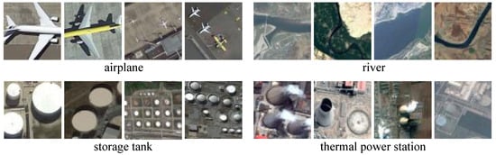
Figure 1.
Diagram of samples in the NWPU-RESISC45 dataset with large differences in the object scales.
To solve this problem, Chen et al. [46] developed the discriminative enhanced attention-based deep nearest neighbor neural network (DEADN4). Initially, the DEADN4 model employs a deep local–global descriptor (DLGD) to perform classification by combining localized and global characteristics, thereby facilitating the distinction between various classes. After this, to strengthen the similarity within the same class, DEADN4 uses a special loss to improve the overall details, bringing features in the same class closer together and reducing the differences within the class. Finally, DEADN4 enhances the accuracy of classification by incorporating a cosine margin into the Softmax loss, making the differences between features from different classes clearer. However, the DEADN4 method does not solve the problem of the large size differences among the objects in the RSI.
To address the abovementioned problem, this paper proposes a two-stream deep nearest neighbor neural network (TSDN4), accomplished by constructing a global–local two-stream network. This network has two parts: the global stream, which looks at the whole image to find out whether it belongs to a certain class, and the local stream, which focuses on the most important part of the image to see whether it falls into a particular class. The final classification result is obtained by combining the results from both parts. To find the most important areas in the image, the key area localization (KAL) method is used to link the two parts mentioned above. Section 2 discusses earlier work within this domain, while Section 3 introduces our proposed method. Next, Section 4 discusses the results of our experiments and analysis. Lastly, Section 6 highlights the main conclusions from our research.
2. Related Work
The method proposed in this paper builds upon DEADN4 [46]; therefore, this section mainly focuses on introducing DEADN4. The primary objective of DEADN4 is to tackle the challenge posed by few-shot RSISC, which comprises two key components: a deep embedding module that utilizes attention mechanisms, denoted as , and a metric module, represented by . The core function of the module is to derive representative details from the images and generate attention maps highly pertinent to the scene class. As for every input image X, the function produces a feature map of the dimensions , comprising DLGD instances, each with d dimensions. A DLGD consists of a deep local descriptor (DLD) and a deep global descriptor (DGD). DLDs extract features from various regions of the image, while the DGD captures the global details, serving as a useful guide to enhance the distinctiveness of each local feature.
Moreover, the module includes a component for acquiring class-distinctive attention capabilities. This component classifies the local features into pertinent and non-pertinent segments according to the scene classification. The main goal here is to minimize the impact of background noise and highlight features that are important to the scene class. Lastly, within the module, the classification of a query image is acquired by contrasting its features with those of the support images.
To summarize, DEADN4 employs the module to derive features pertinent to scene classification from the images, and then the module assesses the feature resemblance between the query and support images to enable RSISC.
The DEADN4 loss function is defined as follows:
where the overall loss includes contributions from the central loss and the class loss , with as a scalar that adjusts the influence of .
The central loss term in Equation (1) can be described as follows:
where C denotes the overall count of classes, K indicates the quantity of instances per class in the support set, is the global feature of the j-th instance within the support set’s i-th class, and denotes the mean global feature across all instances associated with the i-th class in the support set.
The class loss , as mentioned in Equation (1), is defined as follows:
where stands for the likelihood of accurately categorizing the query image, k represents the number of nearest neighbors, m denotes the DLGD’s count, and M serves as an additional margin enhancing the resemblance between descriptors.
3. Methods
3.1. Architecture
To tackle the challenge of significant variations in the objects within images, this paper proposes a method for scene image classification that combines global and local metrics. As shown in Figure 2, a two-stream network that combines both global and local measurements is designed. Within this framework, the network’s blue pathway represents the global stream for measuring the overall image, calculating the resemblance between images and classes. Meanwhile, the network’s green pathway represents the local stream, which focuses on measuring a particular area within the image. It emphasizes the most significant object by focusing on key local areas when calculating the similarities between areas. The two-stream network proposed in this paper allows for separate measurements of the entire image and specific areas from inputs of different sizes, with their classification results eventually being combined.
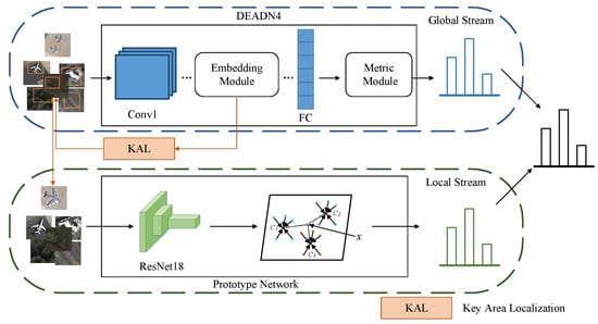
Figure 2.
Diagram of global–local two-stream network.
The global stream uses the DEADN4 model, while the local stream employs a prototype network. To identify the most important local areas within the whole image, this paper further introduces a weakly supervised key area detection method, called KAL, as shown in the path in Figure 2. KAL, using scene-related attention maps, is a clear method for finding key local areas, connecting the two streams. It aims to precisely identify the most significant area and find the coordinates of its bounding box , where and are the left and right edges of the area’s width, and and represent the upper and lower edges of the area’s height.
3.2. Key Area Localization
In an image, finding key areas is the most important step, connecting the global and local streams. The flowchart for the KAL strategy is displayed in Figure 3. Specifically, using the attention maps related to the scene classes from DEADN4, a bounding box is created to help classify the local stream. KAL consists of two sub-steps: vector construction and a greedy boundary search.
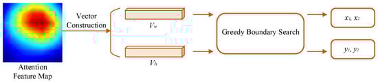
Figure 3.
Flowchart of key area localization method.
3.2.1. Vector Construction
The attention maps related to the scene classes can measure how important each part of an image is. So, using this attention map, we can find areas with high energy, which are the key areas. Because searching in two-dimensional space is complex, in this paper, the attention map is simplified into two one-dimensional energy vectors, one along the height and one along the width of the space, which is formulated as follows:
where is the attention map we obtain, is the value located at position in , the total height is H, and the total width is W. By summing along its height and width, we obtain and , respectively.
To quickly find the most important one-dimensional area in an energy vector, this paper proposes a energy-based greedy boundary search method, which is formulated as follows:
where represents the total energy of all of the components in the width vector , and is the sum of the energies from spatial widths to .
3.2.2. Greedy Boundary Search
This paper defines the key areas in an image as the areas that occupy the minimum space while containing no less than a certain proportion of the overall energy, specifically where , with representing a hyperparameter for the energy ratio. Based on this criterion, a greedy-like algorithm can be employed to search for the most critical areas, which is outlined in Algorithm 1. The greedy boundary search algorithm is described as follows:
| Algorithm 1 Greedy Boundary Search |
| Require: Width vector: |
| Ensure: Width boundaries of the most critical area: |
| for do |
| if then |
| end if |
| end for |
| if then |
| while do |
| if then |
| else |
| end if |
| end while |
| else |
| while do |
| if then |
| else |
| end if |
| end while |
| end if |
Step 1: Initialize and .
Step 2: This involves repeatedly adjusting the limits of to make the energy closer to . After Step 1, two states are possible: the ratio of energy in the area to the total energy in the width direction, , is either higher or lower than . When the ratio is higher than , the area needs to contract in the direction of the slowest energy decrease until the ratio is no longer higher than . On the other hand, when the ratio is lower than , the area must expand in the direction of the fastest energy increase until it is no longer below . This paper’s greedy boundary search can identify the most compact yet informative area.
Step 3: The boundary coordinates are mapped from the feature map to the input image. Since the aforementioned boundary coordinates are located on the feature map, it is necessary to acquire the corresponding coordinates on the image, represented as , where is the coordinate in the width direction on the image, is the coordinate on the feature map, represents the width size of the image, and W indicates the width size of the feature map. The width boundaries of the most critical area in the image, denoted as , can be obtained using the three steps described above. By employing the same algorithm, the height boundaries of the most crucial area, represented as , can similarly be obtained.
3.2.3. The Two-Stream Architecture
The key areas’ positions can be obtained using the KAL module, represented by . The classification results for the global stream are obtained from query and support images inputted into the DEADN4 model, whereas the classification scores of the local stream are generated by utilizing bilinear interpolation to feed the key areas of the query and support images into the prototype network and obtain classification scores. The prototype network is designed to utilize a mapping function that maps input images into a lower-dimensional embedding space, and a prototype representation is learned for each class. Lastly, we compute the distances between the query image’s features and the prototype representation of each class using a standard distance measure for classification purposes. In the prototype network, convolutional neural networks are typically used as the mapping function, with the average of the embedding features for all images within a class being taken as the prototype representation for that class.
Let the mapping function : be defined to transform sample data of the dimension D into an embedding space of the dimension F. The prototype representation for each class is computed as follows:
where represents the dataset for class k, denotes a sample in , and is its corresponding class. The prototype representation corresponds to the mean of all of the embedding features within the support set for the respective class.
For a given query image , the likelihood that the query image falls into class k can be determined as follows:
where denotes the mapping features obtained from the query image through the mapping function, represents the distance function, and the cosine distance is used in this paper for computation. It should be noted that since the cosine distance offers advantages such as directional consistency, scale invariance, suitability for high-dimensional data, computational efficiency, and strong robustness and the global stream also employs the cosine distance for measurement, the cosine distance is adopted here as well for consistency.
Based on the actual labels of the images and the forecasted likelihood distribution, the local stream loss function is formulated as the negative log-probability, expressed using the formula below:
where N signifies the overall count of samples in the query set, and C denotes the overall count of classes in the query set.
3.2.4. The Loss Function
4. Results
4.1. Dataset Description
In the experiments of this paper, the datasets utilized are the NWPU-RESISC45 [47] dataset, the UC Merced [48] dataset, and the WHU-RS19 [49] dataset. To facilitate comparison, the partitioning of the three datasets is the same as that for DLA-MatchNet [27].
4.1.1. The NWPU-RESISC45 Dataset
The NWPU-RESISC45 dataset, originating from Northwestern Polytechnical University in China, comprises a collection of 31,500 images sourced from Google Earth. The images encompass a diverse variety of over 100 countries and territories, created through a combination of satellite imagery, aerial photography, and geographical information. The dataset includes a variety of weather conditions, scene variations, sizes, seasonal settings, and lighting conditions. The images in this dataset typically have resolutions ranging from 30 m to m and are presented in a full color palette, including red, green, and blue. Figure 4 shows 45 distinct scene classes, with each containing a set of 700 images with dimensions of . In the experimental setup, the dataset is partitioned into three parts: a training subset with 25 classes, a validation subset with 10 classes, and a testing subset with another 10 classes.
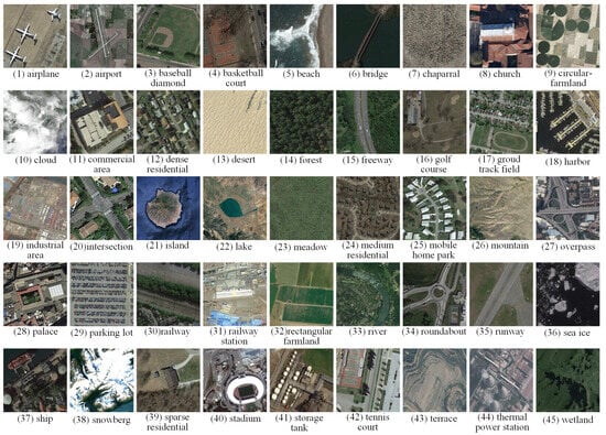
Figure 4.
The NWPU-RESISC45 dataset comprises 45 different scene classes, with each containing 700 images measuring pixels.
4.1.2. The UC Merced Dataset
The UC Merced dataset, introduced in 2010, is based on detailed maps provided by the United States Geological Survey National Map, showcasing a variety of areas in the USA. The RGB dataset maintains a high image resolution of m, spanning 21 varied scene categories. Within this dataset, each of the 21 categories comprises 100 detailed land use images, with each measuring dimensions, as illustrated in Figure 5. To conduct the experiments, the dataset is partitioned into three distinct sets: a training subset with 10 classes, a validation subset with 6 classes, and a testing subset with another 5 classes.
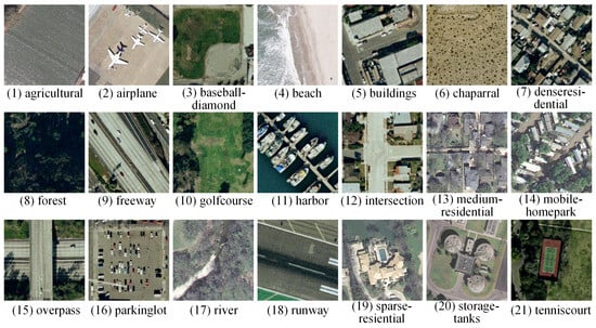
Figure 5.
The UC Merced dataset features 21 unique scene classes, with each containing 100 land use images measuring pixels.
4.1.3. The WHU-RS19 Dataset
Released by Wuhan University in China, the WHU-RS19 dataset is a collection of images sourced directly from the famous Google Earth platform. The RGB dataset employs a fine resolution of m. Displayed in Figure 6, the dataset contains a diverse collection of 19 distinct scene classes. Each of these carefully selected classes contains a minimum of 50 representative samples, with each having a resolution of pixels. The dataset includes a total of 1005 scene images. In the experimental setup, the dataset is partitioned into three distinct parts: a training subset for 9 specific classes, a validation subset for 5 selected classes, and a testing subset comprising another 5 classes.
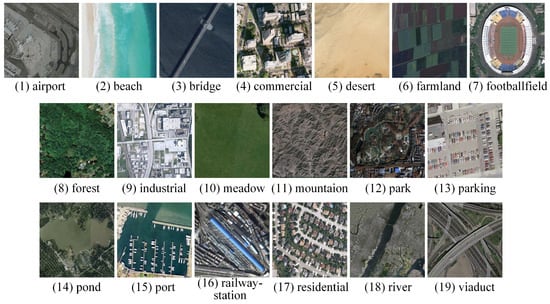
Figure 6.
The WHU-RS19 dataset contains 19 scene classes, each with at least 50 images measuring pixels.
4.2. The Experimental Setting
4.2.1. The Experimental Software and Hardware Environment
The detailed specifications of the software configurations and hardware setups used in this paper are thoroughly presented in Table 1.

Table 1.
The experimental setup included both software and hardware components.
4.2.2. The Experimental Design
We performed experimental evaluations of solving both 5-way 1-shot and 5-way 5-shot problems across the three aforementioned datasets. In order to assess the effectiveness of our method, we benchmarked it against eight well-known few-shot learning methods: MatchingNet [45], RelationNet [50], MAML [51], Meta-SGD [52], DLA-MatchNet [27], DN4 [53], DN4AM [54], and DEADN4 [46]. Given that our method builds upon the DEADN4 framework, we benchmarked it against DEADN4, utilizing an identical embedding network for a fair evaluation. We evaluated the classification results utilizing the mean top-1 accuracy, along with the confidence intervals (CIs), as described in [54].
The global stream of our method adopts the network from DEADN4, while the local stream uses a prototype network, and both streams utilize ResNet18 models for their embedding modules. Random cropping is applied to input images, resizing them to pixels, and these resized images are then subjected to enhancements such as random horizontal flipping, brightness variations, color augmentation, and contrast enhancement. In the classification module, we specify the count of nearest neighbors as , configure the loss function hyperparameter M to , and set the parameter to . The training set comprises 300,000 scenario sets in total, where in the 5-way 1-shot experiment, each scenario set includes 5 support images and 75 query images, while in the 5-way 5-shot experiment, each scenario set includes 25 support images and 50 query images. The Adam [55] algorithm is employed during network training, and the initial learning rate is set to 0.0001. The learning rate undergoes a decay every 100,000 scenarios, and for validation, 600 randomly generated scenario sets are utilized on the validation dataset. The top-performing model’s mean top-1 accuracy is used as the current network’s training outcome, and the model achieving the highest scores is saved as the final version. During the testing phase, we randomly sample 600 scenario sets from the test set five times, calculate the average top-1 accuracy for each iteration, and determine the final testing outcome as the mean of the results obtained from these iterations. Additionally, the CI is provided.
4.3. The Experimental Results
In this paper, corresponding experiments are performed on the three aforementioned datasets, and comparisons are made with other few-shot learning methods. Table 2, Table 3 and Table 4 show the experimental results of various few-shot classification methods on the three datasets.
Table 2.
Comparison of results of various methods tested on the NWPU-RESISC45 dataset.
Table 3.
Comparison of results of various methods tested on the UC Merced dataset.
Table 4.
Comparison of results of various methods tested on the WHU-RS19 dataset.
5. Discussion
From the results in Table 2, Table 3 and Table 4, it is evident that our method outperforms the others across all three datasets, achieving the highest average accuracy. Additionally, when compared to DEADN4, our method demonstrates improvements of varying degrees across all three datasets, particularly a significant enhancement on the UC Merced dataset, with an average increase in accuracy of . The UC Merced test set comprises scene classes with multi-scale characteristics, such as rivers, sparse residential areas, and tennis courts, indicating that our method has effectively addressed the multi-scale challenges in RSISC.
To visually illustrate the efficacy of the KAL method, the localization results on the NWPU-RESISC45 dataset have been visualized, as depicted in Figure 7. Based on the visual outcomes, it is clear that our method accurately locate key areas within the scenes. In the airplane scene, targets of varying sizes can be accurately localized, while objects with slight scale variations in other scenes, such as rivers, storage tanks, thermal power stations, and parking lots, are also successfully located. This, in turn, benefits the classification processes of the local stream.
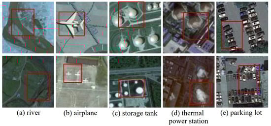
Figure 7.
Localization results for key areas (delineated by red bounding boxes) in some samples from the NWPU-RESISC45 dataset.
6. Conclusions
This paper introduces a few-shot scene classification model utilizing a dual-stream network. Our method constructs a global–local two-stream framework, integrating global and local streams, to calculate the likelihood of a sample belonging to a class by analyzing both the entire image and its most crucial regions. The KAL method is also designed to identify the most crucial areas within the entire image. Our method utilizes a greedy strategy to quickly identify the most critical areas within the overall image while linking the two aforementioned streams. To assess our method’s performance, tests are carried out on three public RSI datasets, and the visual outcomes of the KAL method on the NWPU-RESISC45 dataset are presented. Through a qualitative analysis and ablation experiments, our method can successfully tackle the multi-scale challenge in scene classification for few-shot RSIs. In the context of few-shot RSISC, mislabeled samples significantly impact the classification accuracy, and exploring strategies to mitigate their effects presents a promising direction for future research.
Author Contributions
Methodology, Y.L. (Yaolin Lei), Y.L. (Yangyang Li) and H.M. Resources, Y.L. (Yangyang Li). Software, H.M. and Y.L. (Yangyang Li). Writing, Y.L. (Yaolin Lei). All authors have read and agreed to the published version of the manuscript.
Funding
This work was supported in part by the National Natural Science Foundation of China under Grant No. 62476209, in part by the Key Research and Development Program of Shaanxi under Grant No. 2024CY2-GJHX-18, and in part by the Natural Science Basic Research Program of Shaanxi under Grant No. 2022JC-45.
Data Availability Statement
The NWPU-RESISC45 dataset can be retrieved from [47], the UC Merced dataset accessed via [48], and the WHU-RS19 dataset obtained through [49].
Acknowledgments
The authors express their sincere gratitude to all of the reviewers and editors for the invaluable feedback provided on this paper.
Conflicts of Interest
The authors assert the absence of any conflicts of interest.
Abbreviations
The following abbreviations are used in this manuscript:
| N | sample count per class of the query set |
| K | sample count per class of the support set |
| C | class number |
| metric module | |
| embedding module | |
| c | a specific class |
| feature map | |
| s | constant |
| cosine | |
| central loss of DEADN4 | |
| class loss of EWADN4 | |
| left boundary of the key area width | |
| right boundary of the key area width | |
| upper boundary of the key area height | |
| lower boundary of the key area height | |
| total of the feature map across the width axis | |
| total of the feature map across the height axis | |
| E | energy |
| total loss of DEADN4 | |
| prototype representation | |
| local stream loss of our method | |
| total loss of our method | |
| total loss of our method | |
| constant | |
| constant | |
| p | classification probability |
| H | feature map’s height |
| W | feature map’s width |
| d | size of the DLGD |
| B | bounding box |
References
- Jiang, N.; Shi, H.; Geng, J. Multi-Scale Graph-Based Feature Fusion for Few-Shot Remote Sensing Image Scene Classification. Remote Sens. 2022, 14, 5550. [Google Scholar] [CrossRef]
- Xing, S.; Xing, J.; Ju, J.; Hou, Q.; Ding, X. Collaborative Consistent Knowledge Distillation Framework for Remote Sensing Image Scene Classification Network. Remote Sens. 2022, 14, 5186. [Google Scholar] [CrossRef]
- Xiong, Y.; Xu, K.; Dou, Y.; Zhao, Y.; Gao, Z. WRMatch: Improving FixMatch with Weighted Nuclear-Norm Regularization for Few-Shot Remote Sensing Scene Classification. IEEE Trans. Geosci. Remote Sens. 2022, 60, 5612214. [Google Scholar]
- Bai, T.; Wang, H.; Wen, B. Targeted Universal Adversarial Examples for Remote Sensing. Remote Sens. 2022, 14, 5833. [Google Scholar] [CrossRef]
- Muhammad, U.; Hoque, M.; Wang, W.; Oussalah, M. Patch-Based Discriminative Learning for Remote Sensing Scene Classification. Remote Sens. 2022, 14, 5913. [Google Scholar] [CrossRef]
- Chen, X.; Zhu, G.; Liu, M. Remote Sensing Image Scene Classification with Self-Supervised Learning Based on Partially Unlabeled Datasets. Remote Sens. 2022, 14, 5838. [Google Scholar] [CrossRef]
- Yao, X.; Feng, X.; Han, J.; Cheng, G.; Guo, L. Automatic Weakly Supervised Object Detection from High Spatial Resolution Remote Sensing Images via Dynamic Curriculum Learning. IEEE Trans. Geosci. Remote Sens. 2021, 59, 675–685. [Google Scholar] [CrossRef]
- Huang, X.; Han, X.; Ma, S.; Lin, T.; Gong, J. Monitoring ecosystem service change in the City of Shenzhen by the use of high-resolution remotely sensed imagery and deep learning. Land Degrad. 2019, 30, 1490–1501. [Google Scholar] [CrossRef]
- Zhu, Q.; Zhong, Y.; Zhang, L.; Li, D. Adaptive deep sparse semantic modeling framework for high spatial resolution image scene classification. IEEE Trans. Geosci. Remote Sens. 2018, 56, 6180–6195. [Google Scholar]
- Fang, B.; Li, Y.; Zhang, H.; Chan, J.C.W. Semi-Supervised Deep Learning Classification for Hyperspectral Image Based on Dual-Strategy Sample Selection. Remote Sens. 2018, 10, 574. [Google Scholar] [CrossRef]
- Cheng, G.; Guo, L.; Zhao, T.; Han, J.; Li, H.; Fang, J. Automatic landslide detection from remote-sensing imagery using a scene classification method based on BoVW and pLSA. Int. J. Remote Sens. 2013, 34, 45–59. [Google Scholar] [CrossRef]
- Lv, Z.; Shi, W.; Zhang, X.; Benediktsson, J. Landslide inventory mapping from bitemporal high-resolution remote sensing images using change detection and multiscale segmentation. IEEE J. Sel. Top. Appl. Earth Observ. 2018, 11, 1520–1532. [Google Scholar]
- Longbotham, N.; Chaapel, C.; Bleiler, L.; Padwick, C.; Emery, W.; Pacifici, F. Very high resolution multiangle urban classification analysis. IEEE Trans. Geosci. Remote Sens. 2011, 50, 1155–1170. [Google Scholar] [CrossRef]
- Tayyebi, A.; Pijanowski, B.; Tayyebi, A. An urban growth boundary model using neural networks, GIS and radial parameterization: An application to Tehran, Iran. Landscape Urban. Plan. 2011, 100, 35–44. [Google Scholar] [CrossRef]
- Huang, X.; Wen, D.; Li, J.; Qin, R. Multi-level monitoring of subtle urban changes for the megacities of China using high-resolution multi-view satellite imagery. Remote Sens. Environ. 2017, 196, 56–75. [Google Scholar]
- Zhang, T.; Huang, X. Monitoring of urban impervious surfaces using time series of high-resolution remote sensing images in rapidly urbanized areas: A case study of Shenzhen. IEEE J. Sel. Top. Appl. Earth Observ. 2018, 11, 2692–2708. [Google Scholar]
- Li, X.; Shao, G. Object-based urban vegetation mapping with high-resolution aerial photography as a single data source. Int. J. Remote Sens. 2013, 34, 771–789. [Google Scholar]
- Rußwurm, M.; Körner, M. Multi-temporal land cover classification with sequential recurrent encoders. ISPRS Int. J. Geo-Inf. 2018, 7, 129. [Google Scholar] [CrossRef]
- Othman, E.; Bazi, Y.; Melgani, F.; Alhichri, H.; Alajlan, N.; Zuair, M. Domain adaptation network for cross-scene classification. Remote Sens. 2017, 55, 4441–4456. [Google Scholar] [CrossRef]
- Chaib, S.; Liu, H.; Gu, Y.; Yao, H. Deep feature fusion for VHR remote sensing scene classification. Remote Sens. 2017, 55, 4775–4784. [Google Scholar] [CrossRef]
- Wang, X.; Xu, H.; Yuan, L.; Dai, W.; Wen, X. A remote-sensing scene-image classification method based on deep multiple-instance learning with a residual dense attention ConvNet. Remote Sens. 2022, 14, 5095. [Google Scholar] [CrossRef]
- Gao, Y.; Sun, X.; Liu, C. A General Self-Supervised Framework for Remote Sensing Image Classification. Remote Sens. 2022, 14, 4824. [Google Scholar] [CrossRef]
- Zhao, Y.; Liu, J.; Yang, J.; Wu, Z. Remote Sensing Image Scene Classification via Self-Supervised Learning and Knowledge Distillation. Remote Sens. 2022, 14, 4813. [Google Scholar] [CrossRef]
- Alajaji, D.; Alhichri, H.S.; Ammour, N.; Alajlan, N. Few-Shot Learning For Remote Sensing Scene Classification. In Proceedings of the Mediterranean and Middle-East Geoscience and Remote Sensing Symposium, Tunis, Tunisia, 9–11 March 2020; pp. 81–84. [Google Scholar]
- Noothout, J.M.H.; De Vos, B.D.; Wolterink, J.M.; Postma, E.M.; Smeets, P.A.M.; Takx, R.A.P.; Leiner, T.; Viergever, M.A.; Išgum, I. Deep Learning-Based Regression and Classification for Automatic Landmark Localization in Medical Images. IEEE Trans. Med. Imaging. 2020, 39, 4011–4022. [Google Scholar] [CrossRef] [PubMed]
- Cen, F.; Wang, G. Boosting Occluded Image Classification via Subspace Decomposition-Based Estimation of Deep Features. IEEE Trans. Cybern. 2020, 50, 3409–3422. [Google Scholar] [CrossRef] [PubMed]
- Li, L.; Han, J.; Yao, X.; Cheng, G.; Guo, L. DLA-MatchNet for few-shot remote sensing image scene classification. IEEE Trans. Geosci. Remote Sens. 2020, 59, 7844–7853. [Google Scholar] [CrossRef]
- Simonyan, K.; Zisserman, A. Very deep convolutional networks for large-scale image recognition. arXiv 2014, arXiv:1409.1556v6. [Google Scholar]
- Szegedy, C.; Liu, W.; Jia, Y.; Sermanet, P.; Reed, S.; Anguelov, D.; Erhan, D.; Vanhoucke, V.; Rabinovich, A. Going deeper with convolutions. In Proceedings of the IEEE Conference on Computer Vision and Pattern Recognition, Boston, MA, USA, 7–12 June 2015; pp. 1–9. [Google Scholar]
- Krizhevsky, A.; Sutskever, I.; Hinton, G.E. Imagenet classification with deep convolutional neural networks. Commun. ACM 2017, 60, 84–90. [Google Scholar] [CrossRef]
- He, K.; Zhang, X.; Ren, S.; Sun, J. Deep residual learning for image recognition. In Proceedings of the IEEE Conference on Computer Vision and Pattern Recognition (CVPR), Las Vegas, NV, USA, 27–30 June 2016; pp. 770–778. [Google Scholar]
- Liu, Y.; Zhong, Y.; Fei, F.; Zhang, L. Scene semantic classification based on random-scale stretched convolutional neural network for high-spatial resolution remote sensing imagery. In Proceedings of the IEEE International Geoscience and Remote Sensing Symposium, Beijing, China, 10–15 July 2016; pp. 763–766. [Google Scholar]
- Wu, B.; Meng, D.; Zhao, H. Semi-Supervised Learning for Seismic Impedance Inversion Using Generative Adversarial Networks. Remote Sens. 2021, 13, 909. [Google Scholar] [CrossRef]
- Geng, J.; Deng, X.; Ma, X.; Jiang, W. Transfer Learning for SAR Image Classification via Deep Joint Distribution Adaptation Networks. IEEE Trans. Geosci. Remote Sens. 2020, 58, 5377–5392. [Google Scholar] [CrossRef]
- Zhan, T.; Song, B.; Xu, Y.; Wan, M.; Wang, X.; Yang, G.; Wu, Z. SSCNN-S: A spectral-spatial convolution neural network with Siamese architecture for change detection. Remote Sens. 2021, 13, 895. [Google Scholar] [CrossRef]
- Du, L.; Li, L.; Guo, Y.; Wang, Y.; Ren, K.; Chen, J. Two-Stream Deep Fusion Network Based on VAE and CNN for Synthetic Aperture Radar Target Recognition. Remote Sens. 2021, 13, 4021. [Google Scholar] [CrossRef]
- Xu, P.; Li, Q.; Zhang, B.; Wu, F.; Zhao, K.; Du, X.; Yang, C.; Zhong, R. On-Board Real-Time Ship Detection in HISEA-1 SAR Images Based on CFAR and Lightweight Deep Learning. Remote Sens. 2021, 13, 1995. [Google Scholar] [CrossRef]
- Wang, X.; Wang, S.; Ning, C.; Zhou, H. Enhanced feature pyramid network with deep semantic embedding for remote sensing scene classification. IEEE Trans. Geosci. Remote Sens. 2021, 59, 7918–7932. [Google Scholar] [CrossRef]
- Sun, X.; Wang, B.; Wang, Z.; Li, H.; Li, H.; Fu, K. Research Progress on Few-Shot Learning for Remote Sensing Image Interpretation. IEEE J. Sel. Top. Appl. Earth Obs. Remote Sens. 2021, 14, 637–648. [Google Scholar]
- Wang, Y.; Yao, Q.; Kwok, J.; Ni, L. Generalizing from a few examples: A survey on few-shot learning. ACM Comput. Surv. 2020, 53, 1–34. [Google Scholar]
- Li, X.; Sun, Z.; Xue, J.; Ma, Z. A concise review of recent few-shot meta-learning methods. Neurocomputing 2021, 456, 463–468. [Google Scholar] [CrossRef]
- Snell, J.; Swersky, K.; Zemel, R. Prototypical networks for few-shot learning. Adv. Neural Inf. Process. Syst. 2017, 30, 4080–4090. [Google Scholar]
- Yan, B.; Lang, C.; Cheng, G.; Han, J. Understanding negative proposals in generic few-shot object detection. IEEE Trans. Circ. Syst. Vid. 2024, 34, 5818–5829. [Google Scholar]
- Zeng, Q.; Geng, J.; Huang, K.; Jiang, W.; Guo, J. Prototype calibration with feature generation for few-shot remote sensing image scene classification. Remote Sens. 2021, 13, 2728. [Google Scholar] [CrossRef]
- Vinyals, O.; Blundell, C.; Lillicrap, T.; Wierstra, D. Matching networks for one shot learning. In Proceedings of the Advances in Neural Information Processing Systems, Barcelona, Spain, 5–10 December 2016; pp. 3630–3638. [Google Scholar]
- Chen, Y.; Li, Y.; Mao, H.; Liu, G.; Chai, X.; Jiao, L. A Novel Discriminative Enhancement Method for Few-Shot Remote Sensing Image Scene Classification. Remote Sens. 2023, 15, 4588. [Google Scholar] [CrossRef]
- Cheng, G.; Han, J.; Lu, X. Remote sensing image scene classification: Benchmark and state of the art. Proc. IEEE 2017, 105, 1865–1883. [Google Scholar] [CrossRef]
- Yang, Y.; Newsam, S. Bag-of-visual-words and spatial extensions for land-use classification. In Proceedings of the 18th SIGSPATIAL International Conference on Advances in Geographic Information Systems, San Jose, CA, USA, 2–5 November 2010; pp. 270–279. [Google Scholar]
- Sheng, G.; Yang, W.; Xu, T.; Sun, H. High-resolution satellite scene classification using a sparse coding based multiple feature combination. Int. J. Remote Sens. 2012, 33, 2395–2412. [Google Scholar] [CrossRef]
- Sung, F.; Yang, Y.; Zhang, L.; Xiang, T.; Torr, P.; Hospedales, T. Learning to compare: Relation network for few-shot learning. In Proceedings of the IEEE Conference on Computer Vision and Pattern Recognition (CVPR), Salt Lake City, UT, USA, 18–22 June 2018; pp. 1199–1208. [Google Scholar]
- Finn, C.; Abbeel, P.; Levine, S. Model-agnostic meta-learning for fast adaptation of deep networks. In Proceedings of the International Conference on Machine Learning (ICML), Sydney, Australia, 6–11 August 2017; pp. 1126–1135. [Google Scholar]
- Li, Z.; Zhou, F.; Chen, F.; Li, H. Meta-sgd: Learning to learn quickly for few-shot learning. arXiv 2017, arXiv:1707.09835v2. [Google Scholar]
- Li, W.; Wang, L.; Xu, J.; Huo, J.; Gao, Y.; Luo, J. Revisiting Local Descriptor Based Image-To-Class Measure for Few-Shot Learning. arXiv 2019, arXiv:1903.12290v2. [Google Scholar]
- Chen, Y.; Li, Y.; Mao, H.; Chai, X.; Jiao, L. A Novel Deep Nearest Neighbor Neural Network for Few-Shot Remote Sensing Image Scene Classification. Remote Sens. 2023, 15, 666. [Google Scholar] [CrossRef]
- Kingma, D.; Ba, J. Adam: A Method for Stochastic Optimization. In Proceedings of the International Conference on Learning Representations (ICLR), San Diego, CA, USA, 7–9 May 2015. [Google Scholar]
Disclaimer/Publisher’s Note: The statements, opinions and data contained in all publications are solely those of the individual author(s) and contributor(s) and not of MDPI and/or the editor(s). MDPI and/or the editor(s) disclaim responsibility for any injury to people or property resulting from any ideas, methods, instructions or products referred to in the content. |
© 2025 by the authors. Licensee MDPI, Basel, Switzerland. This article is an open access article distributed under the terms and conditions of the Creative Commons Attribution (CC BY) license (https://creativecommons.org/licenses/by/4.0/).