Deep Learning and Hydrological Feature Constraint Strategies for Dam Detection: Global Application to Sentinel-2 Remote Sensing Imagery

Abstract

Dams are instrumental in flood and drought control, agricultural irrigation, and hydropower generation. Remote sensing imagery enables the detection of dams across extensive areas, thereby supplying valuable data to facilitate effective water resource management. However, existing dam detection methods cannot achieve high-precision and rapid detection of dams in medium-resolution remote sensing images at the global scale. To fill the gap, deep learning and hydrological feature constraint strategies (DL-HFCS) for dam detection in Sentinel-2 MSI imagery were proposed. This method leverages the efficient YOLOv5s model for preliminary deep learning-based dam detection. Next, based on the hydrological features of dams, constraints such as adjacent water body, single reservoir-based dam number, watershed river network, and detection box-based river network elevation difference are progressively introduced to eliminate false detections. To verify the effectiveness and generalization of our method, 91 1° × 1° regions worldwide were selected as test areas to conduct dam prediction experiments. Experimental results demonstrate that the DL-HFCS achieves a precision of 86.29% and a recall of 82.26%, a 47.58% improvement in precision compared to deep learning alone. Furthermore, over 98% of the detection results accurately locate the dam bodies, whereas in existing dam datasets, this proportion is less than 75%. This study indicates that the HFCS can effectively reduce the false alarm in dam detection. The DL-HFCS method enables thorough and accurate dam detection on a global scale. It holds significant potential for application to Sentinel-2 MSI imagery worldwide, thereby facilitating the creation of a global dam dataset.

1. Introduction

Dams are one of the oldest and most important water infrastructures, benefiting various aspects such as water supply, irrigation, power generation, and flood control, with substantial socio-economic impacts [1,2,3,4]. A comprehensive and accurate dam dataset is essential for assessing global-scale dam construction’s impact on hydrological processes, water resource redistribution, ecological environments, and climate change [5,6,7,8]. However, existing global dam datasets exhibit geographical position deviation and limited coverage, hindering the assessment [9]. Therefore, achieving comprehensive and accurate global dam remote sensing detection and mapping is crucial. As a key technology, satellite remote sensing has developed over several decades. It offers advantages such as extensive spatial coverage, short revisit cycles, and low costs [10]. However, a global dam dataset constructed via deep learning-based detection has not been released [11], primarily due to a lack of research on related methods. Therefore, it is necessary and urgent to develop a dam detection method tailored to Sentinel-2 MSI imagery, with the potential for global-scale application.

In recent years, with the advent of artificial intelligence [12,13,14,15], dam detection methods have gradually shifted from traditional edge detection and manual detection to deep learning-based object detection. Edge detection constructs discriminative criteria based on the geometric features of the up and downstream edges of dams, which are approximately parallel, to detect dams in water bodies [16]; manual detection involves inspecting high-resolution remote sensing images and annotating dams [9]; deep learning-based object detection methods refer to inputting remote sensing imagery into a well-trained deep learning model, automatically performing multi-level feature extraction to identify and locate dams [17].

Manual detection is generally used for constructing dam datasets, such as GranD [18], GeoDAR [19], GOODD [20], GDAT [21], and so on [9,22,23,24,25,26]. The accuracy of dam location can be guaranteed by referencing high-resolution remote sensing imagery to validate and refine existing dam catalogs. In object detection, Fang was the first to apply the HRLibra-RCNN model to detect dams in Google Earth’s 5 m resolution imagery, achieving an average precision of 79.4% across seven global regions [17]. Jing, building upon the application of multiple YOLO models for dam detection, introduced terrain-sensitive indices and land cover data for geographical constraints, successfully detecting 112 out of 140 dams in the experimental area, with a precision of 80% and a recall rate of 91.06% [27,28]. Jing fused convolutional neural networks (CNNs) and self-attention mechanisms to propose a dam detection and segmentation method named YOLOv5s-ViT-BiFPN [29]. In two experimental areas, the recall rates reached 69.2% and 81.5%, respectively. Wang compared the performance of multiple deep learning models for dam detection in high-resolution remote sensing imagery and proposed a three-stage spatial constraint strategy. This strategy includes hydrological analysis, terrain analysis, and the dam detection ratio method (DDRM) [30]. Using this strategy, the Cascade R-CNN + SCS model achieved the highest accuracy, with a precision of 88% and a recall exceeding 94%. The two-stage Bilinear-CNN and NIR-RCNN proposed by Zhang, when applied to Sentinel-2 remote sensing imagery, can detect the majority of dams, achieving a recall rate of 80.83% and a precision of 40.56% [31].

There are still several issues in current dam detection methods: (1) In edge detection, dam edges are influenced by seasonal fluctuations in water bodies, leading to significant variations in detection results across seasons. In addition, the geometric shape of dams can easily be confused with other structures, such as bridges [16]. (2) In manual detection, the accuracy is highly dependent on the observer’s dam expertise. Different observers may have varying interpretations of the dams, especially when the boundaries of the features are unclear or the image quality is poor. Consequently, scaling up this method to a global scale becomes time-consuming and labor-intensive. (3) Existing AI-based dam detection studies are generally limited to small or specific regions and primarily utilize high-resolution remote sensing imagery. Whether these methods are equally effective when applied to larger areas remains unclear. Some studies suggest that the detection performance may degrade with the expansion of the study area [28]. In the context of medium-resolution imagery, dam detection accuracy is often unsatisfactory, and manual verification is required before practical application [31]. Additionally, current dam detection methods primarily utilize RGB (Red, Green, Blue) bands [32], ignoring dams’ reflection characteristics in multispectral bands. (4) In geographic or spatial constraint methods, false detections are removed based on terrain-sensitive indices such as undulation and roughness [28,30]. However, in cross-regional applications, these methods encounter issues such as limited applicability and reduced accuracy, necessitating a redesign of the constraint.

To address the shortcomings of existing methods, we propose a novel dam detection method based on Sentinel-2 imagery, which integrates deep learning and hydrological feature constraint strategies (DL-HFCS). Numerous test areas were selected on a global scale to validate the effectiveness of our method, ensuring a comprehensive assessment. The structures of this paper are constructed as follows. Section 2 provides a detailed description of the DL-HFCS framework; Section 3 introduces the data used and specific experimental procedures; Section 4 and Section 5 present and discuss the experimental results; Section 6 concludes the paper.

2. DL-HFCS

2.1. Deep Learning

2.1.1. Deep Learning Model

In recent years, advancements in deep learning have spurred the development of intelligent models for detecting ground objects (e.g., airports and ships), enabling the rapid and accurate extraction of target features from large-scale remote sensing images [33,34]. These models can be broadly categorized into two types: (1) single-stage models, such as YOLO and SSD [35,36], which directly predict bounding boxes and categories without generating candidate regions. These models are computationally efficient and fast but tend to have relatively lower detection accuracy; (2) two-stage models based on “region proposal and fine regression”, such as Faster R-CNN [37], which achieve higher accuracy at the cost of computational complexity. Additionally, Transformer-based architectures like DETR and RT-DETR leverage self-attention mechanisms to extract global context [38], eliminating the need for traditional non-maximum suppression (NMS) in post-processing. However, these models heavily rely on large training data. Overall, a significant trade-off exists among speed, accuracy, and resource requirements across different models. In large-scale remote sensing images, where most of the image area does not contain targets such as dams, selecting an object detection model that balances both high speed and accuracy becomes critically important.

The YOLOv5 deep learning model is chosen to detect dams in Sentinel-2 imagery. YOLOv5 is a single-stage object detection model capable of directly locating and classifying targets within input images [39]. Featuring high accuracy, fast processing speed, and low computational cost, it is suitable for detecting dams on large spatial scales [28]. YOLOv5 offers multiple versions, including Nano, Small, Medium, Large, and Extra Large, with differences in parameter size and computational complexity. Considering the limitations of computational resources, the YOLOv5s version is selected. The key architecture of YOLOv5s comprises three components, which are the backbone, neck, and head (Figure 1). The backbone uses the lightweight CSPDarknet to enhance feature extraction capabilities [40], the neck improves detection performance for targets of diverse sizes through multi-scale feature fusion, and the head introduces the CIOU loss function to enhance localization accuracy.

2.1.2. Band Combinations of Dam Samples

Dams are typically located adjacent to reservoirs. Selecting band combinations that highlight both the spectral features of the dam and the water body helps the model better learn their characteristics, thereby improving detection accuracy [41]. In RGB bands, the dam appears as white strips or arcs, exhibiting a distinct spectral difference from the surrounding features, with houses, white clouds, and snow showing similar reflectance. In SNR (SWIR, NIR, Red) bands, the water appears deep black, with shadows having similar reflectance, making it easy to distinguish from the dam.

In RGB bands, factors such as vegetation cover may interfere with the spectral characteristics of the dam, making them more challenging to detect. In contrast, despite these interferences, dams can still be effectively detected in SNR bands due to the significant reflectance difference between the dam and the water body. However, the detection capability of the SNR bands diminishes when the water level is low or water turbidity is high. Additionally, the SNR bands mistakenly detect riverbanks or bunds during the tillering stage as dams. Therefore, this study trains the YOLOv5s model using a Sentinel-2 dam sample dataset based on two band combinations, RGB and SNR (Figure 1), to reduce the miss and false rates.

2.1.3. Models Training and Detection

During the training phase, YOLOv5s automatically performs data augmentation operations on the training set, including random flipping, cropping, rotation, and mosaic stitching, to improve the model’s generalization ability and accelerate convergence. In addition, YOLOv5s employs an automatic anchor technique that generates or fine-tunes anchors based on the distribution of target boxes in the training set. After training, the YOLOv5s (RGB) model for the RGB bands and the YOLOv5s (SNR) model for the SNR bands were obtained (Figure 1).

In the dam detection stage, Sentinel-2 imagery is divided into RGB and SNR band combinations and input into the models. The output includes detection boxes and confidence scores. The detection boxes represent the locations of the dams detected by the model, while the confidence score reflects the probability that the location is a dam. The detection results from both models are then merged (Figure 2) and vectorized into rectangular boxes.

2.2. Hydrological Feature Constraint Strategies

Although the training samples employ a combined strategy of two different band combinations, RGB and SNR, which significantly reduces the likelihood of miss detection, many features—such as houses, bunds, ponds, and clouds, still exhibit spectral characteristics similar to dams, which could result in a high rate of false alarms. It is well-known that dams possess four hydrological characteristics, including adjacent to reservoirs, with smaller reservoirs generally having one dam and larger reservoirs having multi-dams, situated within river networks, and a significant elevation difference exists between the up and downstream river sections of the dam. To minimize interference from other features and improve accuracy, we proposed a four-stage feature constraint strategy: adjacent water body constraint, single reservoir-based dam number constraint, watershed river network constraint, and detection box-based river network elevation difference constraint. The core concepts and implementation steps of each constraint are as follows.

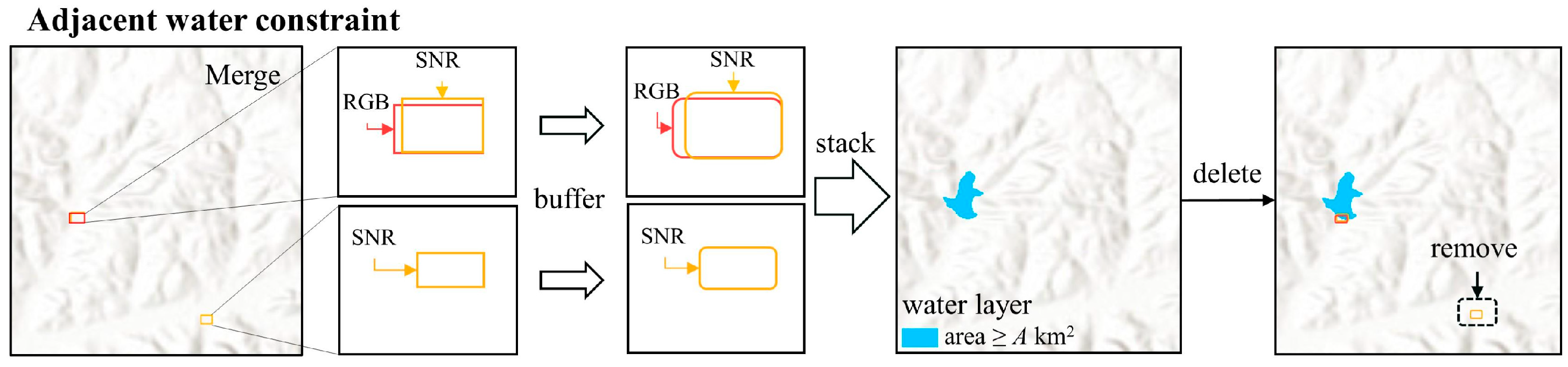
2.2.1. Adjacent Water Body Constraint

Dams, as essential water infrastructures, are typically constructed in large natural water bodies. Therefore, water bodies with area (≥A km²) are selected as references. The dam detection boxes are then evaluated to determine whether they are located within these larger water bodies. Due to seasonal fluctuations in water body boundaries, applying an appropriate buffer to the dam detection box can ensure its intersection with the water body, thereby reducing missed detections. A buffer of B meters is applied to the dam detection box. If the buffered detection box intersects with a water body, it is retained and assigned the corresponding water body ID; otherwise, it is discarded (Figure 3). The retained boxes will subsequently undergo additional constraints to optimize the detection results.

2.2.2. Single Reservoir-Based Dam Number Constraint

Large reservoirs often contain multi-dams, which can be classified into main and auxiliary dams based on their function [19]. Auxiliary dams are located a considerable distance from the main dam to ensure efficient flood discharge and reduce the risk of dam failure during sudden flood events. Terrain conditions influence this distance, ranging from hundreds of meters to a few kilometers.

Meanwhile, smaller reservoirs typically have only one dam. Therefore, a threshold of C km² is used to distinguish between reservoir sizes. When the water area of reservoir ≥ C km², there can be two dams; otherwise, only one dam can exist. To retain auxiliary dams and reduce false detections in large reservoirs, the single reservoir-based dam number constraint is applied to detection boxes sharing the same water body ID (Formula (1)).

$$save=\left\{\begin{array}{ll}da{m}^{1st},& \mathrm{if}A\left(W\right)<C{ \mathrm{km}}^2\\ da{m}^{1st},& \mathrm{if}A\left(W\right)\ge C{ \mathrm{km}}^2,& dist(da{m}^{1st},da{m}^{2nd})<D \mathrm{m}\\ da{m}^{1st} \mathrm{and} da{m}^{2nd},& \mathrm{if}A\left(W\right)\ge C{ \mathrm{km}}^2,& dist(da{m}^{1st},da{m}^{2nd})\ge D\mathrm{m}\end{array}\right.$$

(1)

where A(W) represents the water area of reservoir. dam^1st and dam^2nd are the top two boxes with the highest confidence scores, and dist(dam^1st, dam^2nd) is the distance between them. For small reservoirs (<C km²), if multiple boxes intersect, only dam^1st is retained (Figure 4a). For larger reservoirs (≥C km²), besides dam^1st, dam^2nd will also be retained if the distance between them is at least D m (Figure 4b). All other detection boxes are discarded by default.

2.2.3. Watershed River Network Constraint

Dams are typically located at river confluences with high flow rates to provide sufficient hydraulic resources. Since river networks reflect the characteristics of surface water flow and distribution [42], they can be used to determine whether a detection box meets the required conditions.

In the watershed river network constraint, the river network is first generated based on AW3D30 (Figure 5a–d). The specific steps are as follows. (1) Use fill to fill the missing or anomalous elevation values in AW3D30; (2) Use flow direction to determine the flow direction of each pixel in AW3D30; (3) Use flow accumulation to calculate the runoff for each pixel and select pixels with runoff ≥ 100; (4) Assign stream order (Shreve’s order) to the pixels [43]. If the detection box contains no river network, discard it. If multiple river networks are included, only the river network with the highest catchment capacity will be retained (Formula (2)).

$$B_i=\underset{B_j\in G}{\mathrm{argmax}}(b_j,L_j)$$

(2)

where B_i represents the selected river network, G is the set of all river networks, b_j is the number of branches in river network B_j, and L_j is the total length of B_j. If only one river network is in the detection box, keep it. With multiple river networks, prioritize those with the most branches (Figure 5e–g). If the number of branches is the same, only the network with the longest length is retained (Figure 5h–j).

2.2.4. Detection Box-Based River Network Elevation Difference Constraint

The watershed river network constraint ensures the detection box is located in areas with high flow rates. However, further evaluation is needed to determine whether the water body can flow from the upstream reservoir through the dam to the downstream [9], excluding potential false detections, such as ponds and bunds. The elevation difference constraint was introduced based on the river network.

The detection boxes are classified into two categories based on the number of river network branches. (1) For river networks with multi-branch (≥ 3), the branches are divided into upstream branch sets and downstream branches based on river network ranking. The downstream branch has the highest rank, and the rest belong to the upstream branch set. If the total water-body intersection ratio of the upstream branch set is greater than or equal to the water–body intersection ratio of the downstream branch, the detection box is retained (Formula (3), Figure 6a).

$$save=\left\{{\displaystyle \sum _{i=1}^{n_u}\frac{l(b_{ui}\cap water)}{l(b_{ui})}}\ge {\displaystyle \frac{l(b_d\cap water)}{l(b_d)}},{ b}_{ui}\in {\mathit{Upstream},b}_d\in \mathit{Downstream}\right.$$

(3)

where Upstream represents the upstream branch set, Downstream represents the downstream branch, n_u is the number of upstream branches, b_ui is the i-th upstream branch, b_d is the downstream branch, l(b_ui ∩ water) is the length of the upstream branch i intersecting with water, l(b_ui) is the length of the upstream branch i. Similarly, l(b_d ∩ water) is the length of the downstream branch intersecting with water, and l(b_d) is the length of the downstream branch.

(2) For river networks with only one branch, the water body may be located upstream or downstream, and it is difficult to determine whether there is a dam in the detection box. To address this issue, DSM elevation data were introduced to analyze the water and land parts within the detection box further. Specifically, when the maximum elevation of the water part exceeds the median elevation of the land part, water flows toward the land part, thereby classifying the water body as upstream reservoir water and retaining the detection box (Formula (4), Figure 6b); conversely, the detection box is discarded.

$$save=\left\{max(H_{water})\ge \mathit{median}(H_{land})\right.$$

(4)

where H_water represents the elevation distribution of the water body part, H_land represents the elevation distribution of the land part, max(H_water) is the maximum elevation of the water part, and median(H_land) is the median elevation of the land part.

3. Global Experiments

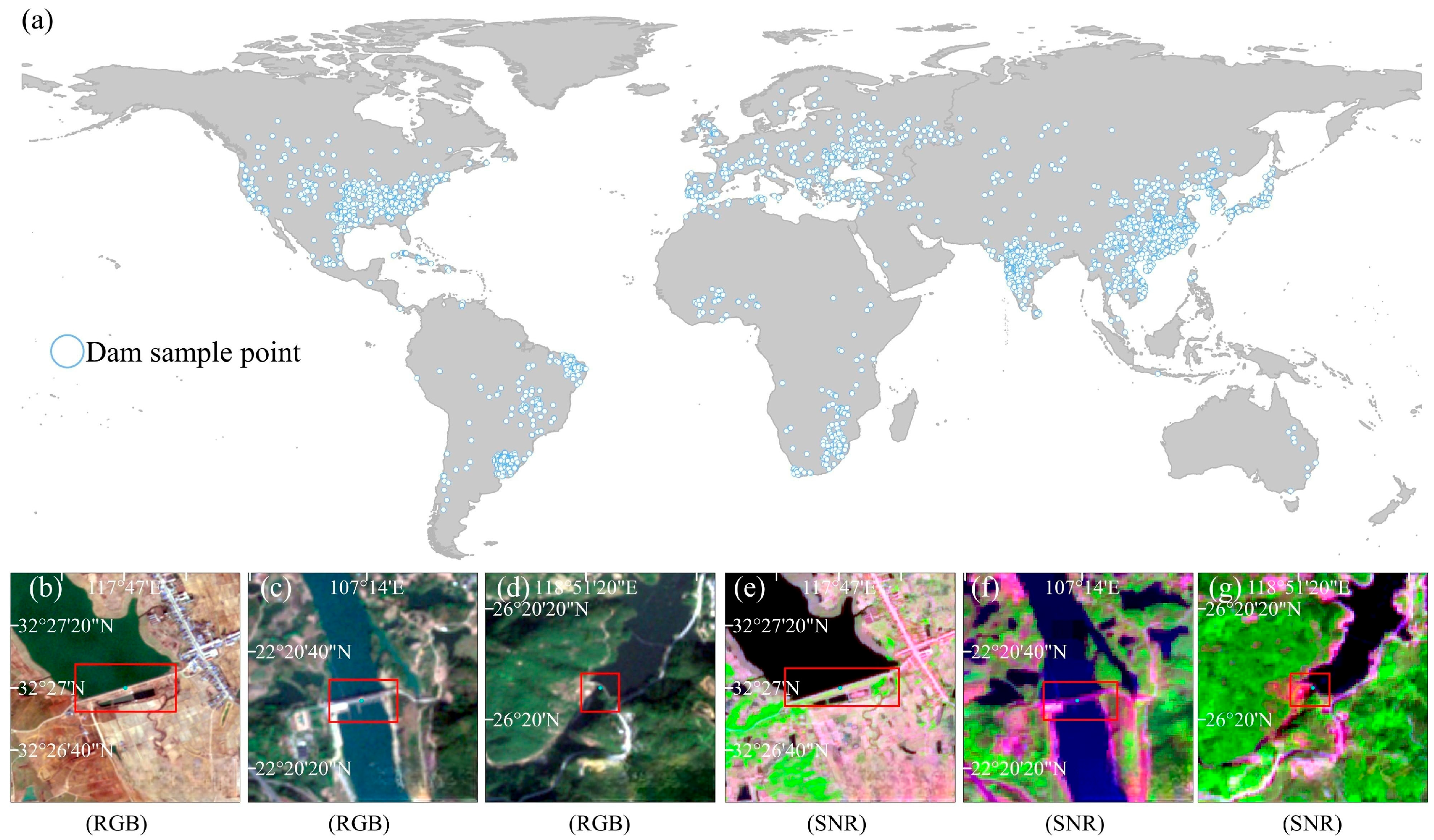
3.1. Test Area

To test the operability and reliability of DL-HFCS for global-scale dam detection, we first trained the model using the sample set and validated its accuracy. Subsequently, several non-overlapping regions were selected for DL-HFCS prediction experiments. The selection method for these test areas is constructed as follows. First, kernel density analysis is performed on the GOODD dam dataset to generate a global dam density map; second, based on this density map, areas with higher dam density were prioritized as test areas. Following this procedure, 91 test areas of 1° × 1° were selected globally (Figure 7), covering a total area of approximately 1.16 × 10⁶ km².

3.2. Data Used

3.2.1. Sentinel-2 MSI Imagery

The remote sensing imagery used for dam detection is Sentinel-2 MSI imagery. Sentinel-2 MSI imagery provides 13 spectral bands from visible light to shortwave infrared, with a spatial resolution of 10–60 m and a revisit cycle of 5 days. All the images were acquired from the Google Earth Engine (GEE) platform, and the selected bands include Red (B4), Blue (B3), Green (B2), Near Infrared (B8), and Shortwave Infrared (B12). In these bands, the reflectance of water is near zero in the near-infrared (827–857 nm) and shortwave infrared (2170–2190 nm).

Considering that some regions have high cloud cover, which results in significant cloud pixels in the images and affects the completeness of dam detection, this study selected all Sentinel-2 images 2021 in test areas with a cloud cover of less than 20% for compositing. The CDI algorithm was then applied for cloud and shadow removal, ensuring image quality and spatial coverage integrity [44]. In the composite Sentinel-2 image, the reflectance of surface features concentrates at the lower end of the sensor’s range, leading to low contrast and unclear details in the imagery [45]. A 2% linear stretch is further applied to enhance surface features’ discernibility. Among the selected bands, except for the shortwave infrared band, which has a spatial resolution of 20 m, the rest have a spatial resolution of 10 m. During the image export process, the shortwave infrared band is resampled to 10 m resolution using the default nearest-neighbor interpolation method.

3.2.2. Google Earth High-Resolution Imagery

Google Earth imagery is sourced from multiple satellite platforms, including Landsat, WorldView series, and GeoEye-1, with spatial resolution ranging from 0.31 m to 30 m [46,47]. Compared to the 10 m spatial resolution of Sentinel-2 imagery, Google Earth’s high-resolution imagery provides more detailed surface features, making it easier to identify dams visually. The Google Earth imagery used has a spatial resolution of 1 m. It was primarily employed to construct the Sentinel-2 MSI imagery-based dam sample dataset and annotate dams in the 91 test areas.

3.2.3. AW3D30 DSM

The AW3D30 Digital Surface Model (DSM) is derived from ALOS satellite observations between 2006 and 2011, with a spatial resolution of 1 arc second (approximately 30 m) and a vertical resolution of 5 m. In areas with a terrain slope of less than 20 degrees, its vertical error is less than 3 m [48,49]. This study primarily used the AW3D30 DSM data to generate the river networks for the 91 test areas.

3.2.4. ESRI Land Use and Land Cover (LULC)

The ESRI Land Use/Land Cover (LULC) product used is consistent with the image acquisition year from 2021, with a spatial resolution of 10 m [50]. During production, this product uses semantic segmentation technology to detect multi-temporal Sentinel-2 images throughout the year. It applies a weighted mode method for pixel-level classification, achieving a high overall classification accuracy [51]. The accuracy for water body classification is 93%. This study used the 2021 ESRI Land Use/Land Cover (LULC) product to extract water body data for the 91 test areas.

3.2.5. Global Dam Datasets

The global dam datasets used include GeoDAR, GOODD, and GDAT. GeoDAR provides geographic coordinates for 24,783 dam locations worldwide, GOODD offers 38,667 dam locations and corresponding reservoir vector boundaries globally, and GDAT provides geographic locations and watershed information for 35,140 dams. These three dam datasets are reference data for selecting samples when constructing the dam sample dataset.

3.3. Methods

3.3.1. Construction of Dam Sample Datasets

Publicly available dam samples are mainly high-resolution satellite or aerial images [52,53]. Models trained using such samples perform dam detection on Sentinel-2 imagery poorly. Therefore, constructing a new Sentinel-2-based dam sample dataset is necessary, following these steps:

(1) Determining dam sample points. Given the enormous global scale and the vast number of Sentinel-2 MSI images, visually identifying dams from individual images is time-consuming and labor-intensive. The potential dam sample points were selected using three global dam datasets (GeoDAR, GOODD, and GDAT). The criteria for selecting dam sample points are listed as follows. The number of dam sample points should not be less than 3000 to ensure sufficient convergence during the training of the YOLOv5s model; regions with higher dam density are selected with more sample points to ensure that the sample distribution aligns with actual conditions. Finally, 4502 dam sample points distributed globally were selected. Based on Sentinel-2 MSI imagery and Google Earth high-resolution imagery, the locations of these 4502 dam sample points were manually corrected to eliminate positional deviation from the actual dam locations, thereby forming a precise dam point distribution map (Figure 8a).

(2) Creating dam sample images. Centered on the selected 4502 dam sample points, boundary boxes of 5000 m × 5000 m were generated, and Sentinel-2 images within these boundary boxes were cropped, resulting in a total of 2761 images with bands including SWIR, NIR, Red, Green, and Blue. The sample images, each approximately 500 × 500 pixels, are divided into RGB and SNR bands. Dams in the Sentinel-2 images were annotated in rectangular boxes on the MakeSense.ai platform. During annotating, the rectangular boxes must enclose the dam outlines to capture their geometric and spectral features fully. Additionally, the rectangular boxes were expanded toward the water bodies to fully utilize the spectral differences between dams and adjacent water bodies. This expansion ensured that the boxes included water bodies (Figure 8b–g).

(3) Augmenting dam sample images. This study applied data augmentation techniques, including vertical flipping, horizontal flipping, and multi-angle rotation, to the 2761 sample images of each band combination. The number of sample images for RGB and SNR band combinations was each expanded to six times the original number, resulting in a dam sample dataset (RGB) and dam sample dataset (SNR), each containing 16,566 images, with a total of 33,132 dam sample images.

3.3.2. Dam Detection Using DL-HFCS

This detection was conducted in PyTorch 2.4 framework, running on an NVIDIA GeForce 1650s graphics card (GPU) (Nvidia, Santa Clara, CA, USA).

In the YOLOv5s model training, 80% of the dam sample datasets (RGB and SNR) are the training set, with 13,248 training samples for each dataset. The remaining 20% of the datasets are the validation set, with 3318 samples. The initial hyperparameter settings are shown in

Table 1. Hyperparameter settings for deep learning models in different band combinations.

Model	Optimizer	Learning Rate	Momentum	Weight Decay	Epochs	Batch Size
YOLOv5s (RGB)	SGD	0.01	0.937	0.0005	200	8
YOLOv5s (SNR)	SGD	0.01	0.937	0.0005	200	8

. Finally, YOLOv5s (RGB) and YOLOv5s (SNR) models were generated.

The model training and validation processes were integrated and conducted simultaneously. At the end of each training epoch, the model is validated using the validation samples to assess its recognition performance on unseen data. By calculating accuracy evaluation metrics for the validation samples, hyperparameters can be adjusted during training to prevent overfitting effectively.

To avoid image distortion and reduce resource consumption, the Sentinel-2 images corresponding to the 91 test areas, each sized 11,333 × 11,333 pixels for both RGB and SNR band combinations, are clipped into non-overlapping tiles of 500 × 500 pixels. These tiles are then input into the trained YOLOv5s (RGB) and YOLOv5s (SNR) models. The dam detection results from both models are merged to obtain the DL stage dam detection results and then vectorized for further constraints.

Based on the DL stage dam detection results, the following Hydrological Feature Constraint Strategies (HFCS) are sequentially applied, including adjacent water constraint, single reservoir-based dam number constraint, watershed river network constraint, and detection box-based river network elevation difference constraint.

In adjacent water body constraint, the parameter A is set to 0.05 km² considering the definition of dams in GOODD and the spatial resolution of Sentinel-2 imagery. Since reservoir water body boundaries fluctuate seasonally, the buffer boundary parameter B is set at 20 m to reduce miss detections caused by the adjacent water body constraint. In the single reservoir-based dam number constraint, the parameter C is set to 1 km² because when the reservoir area exceeds 1 km², multi-dams can be constructed to alleviate water storage pressure. The parameter D is set to 500 m because the distance between auxiliary dams and main dams should not be too close; otherwise, it would reduce the flood discharge efficiency of auxiliary dams. A distance of 500 m is a conservative choice.

In processing the adjacent water body constraint, the dam detection boxes are first buffered outward by 20 m and then intersected with water body data having an area ≥ 0.05 km². Buffered detection boxes that do not intersect with water bodies are discarded, while those that intersect with water bodies are assigned the water body ID. The detection boxes mentioned below are all buffered detection boxes.

Single reservoir-based dam number constraint. No further action is needed for detection boxes with a unique water body ID, which are all retained. For detection boxes with the same water body ID, when the water body area is ≥1 km², they are sorted by confidence, and the two boxes with the highest confidence are selected for subsequent operations. If the distance between both is ≥500 m, retain both. Conversely, if the distance is less than 500 m, only the detection box with the highest confidence level will be retained. When the water body area is <1 km², the detection box with the highest confidence is retained.

Watershed river network constraint. First, detection boxes that do not contain river networks are discarded. In cases where multiple river networks exist within a box, filtering is based on the number of branches and the total branch length, only retaining the river network with the highest catchment capacity.

Detection box-based river network elevation difference constraint. First, detection boxes are categorized based on the number of branches, dividing them into those with multi-branches and those with one branch. Boxes with multi-branches are first divided into upstream branch sets and downstream branches based on branch ranking. Subsequently, water body data are introduced, and the intersection ratios of water bodies for each branch are calculated. If the upstream branch set’s total water body intersection ratio is less than the water body intersection ratio of the downstream branch, the detection box is discarded; otherwise, the detection box is retained.

For detection boxes with one branch, after introducing water body data, the boxes are divided into water and land parts. The elevation distributions of these two parts are then analyzed using AW3D30. If the maximum elevation value of the water part is greater than or equal to the median elevation value of the land part, retain the detection box; otherwise, discard it. All retained buffered detection boxes satisfy the HFCS.

3.3.3. Dam Detection Accuracy Evaluation

The prediction set used to evaluate the dam detection accuracy in the 91 1° × 1° test areas is obtained through manual annotation. The creation process includes two steps. First, filter all water bodies with an area ≥ 0.05 km²; second, inspect water bodies using Google Earth high-resolution imagery. Upon identification of a dam within a water body, it is annotated using a rectangular bounding box. A total of 12,038 actual dams associated with reservoirs having an area ≥ 0.05 km² were annotated.

The evaluation metrics for dam detection performance include precision, recall, F1 score, and mAP@0.5. Precision represents the proportion of correct detection boxes to the total number of detection boxes, recall represents the proportion of correct detection boxes to the total number of dams, and the F1 score is the harmonic mean of precision and recall, serving as a comprehensive evaluation metric. AP is the area under the recall–precision curve. Their calculation formulas are as follows:

$$\mathrm{Precision}={\displaystyle \frac{TP}{TP+FP}}$$

(5)

$$\mathrm{Recall}={\displaystyle \frac{TP}{TP+FN}}$$

(6)

$$\mathrm{F}1={\displaystyle \frac{2\times \mathrm{Precision}\times \mathrm{Recall}}{\left(\mathrm{Precision}+\mathrm{Recall}\right)}}$$

(7)

$$\mathrm{AP}={\displaystyle {\int }_0^1\mathrm{Precision}(r)dr}$$

(8)

where TP represents the number of correct detection boxes, FP represents the number of false detection boxes, and FN represents the number of dams that were not detected.

4. Results

4.1. Dam Detection Accuracy Using Deep Learning

4.1.1. Validation Set

Figure 9 shows the precision and recall value trends on the validation set during the training process of YOLOv5s (RGB) and YOLOv5s (SNR). The YOLOv5s (RGB) model converges after approximately 170 training epochs, achieving a precision of 81.0%, a recall of 73.4%, and mAP@0.5 of 69.9%. Similarly, the YOLOv5s (SNR) model also converges at 170 epochs, with a precision of 81.9%, a recall of 71.1%, and mAP@0.5 of 76.1%. The YOLOv5s (SNR) model performs slightly better than the YOLOv5s (RGB) model in the dam detection task.

To further evaluate the reliability of the YOLOv5s model in dam detection, we conducted a multi-dimensional comparative experiment involving four state-of-the-art detectors: YOLOv11n, RT-DETR [38], DEYOLO [54], and YOLOv5s (SNRGB). Each detector used distinct input strategies and was assessed based on precision, recall, F1 score, and mAP@0.5. YOLOv11n and RT-DETR both used (RGB) and (SNR) band combinations for training. In contrast, YOLOv5s (SNRGB) constructed images with the SNRGB band combination and directly input them into the model for training. DEYOLO, a dual-branch network model, extracted the near-infrared band and combined it with the RGB bands for joint training. The results are summarized in

Table 2. Comparison of training results of different models.

Model	Precision (%)	Recall (%)	F1 (%)	mAP@0.5 (%)
YOLOv5s (RGB)	81.0	73.4	77.0	69.9
YOLOv5s (SNR)	81.9	71.1	76.1	76.1
YOLOv11n (RGB)	66.4	63.3	64.8	60.8
YOLOv11n (SNR)	73.8	60.9	66.7	71.9
RT-DETR (RGB)	73.6	66.2	69.7	60.3
RT-DETR (SNR)	80.7	77.3	79.0	77.3
DEYOLO	72.8	59.6	65.5	64.6
YOLOv5s (SNRGB)	81.8	55.6	66.2	71.0

.

The data in Table 2 highlight the robust performance of YOLOv5s, which maintains high precision across various band combinations. While RT-DETR (SNR) delivers the strongest overall results, achieving a mAP@0.5 of 77.3%, its performance with RGB bands is significantly weaker. YOLOv11n and DEYOLO, on the other hand, show relatively lower performance across all metrics, indicating that further optimization is needed to enhance their accuracy in dam detection.

4.1.2. Prediction Set

In the 91 1° × 1° test areas, the YOLOv5s (RGB) model achieved a precision of 42.78% and a recall of 73.19%, while the YOLOv5s (SNR) model achieved a precision of 35.78% and a recall of 84.14% (

Table 3. Dam detection accuracy of YOLOv5s models in different band combinations.

Model	Precision (%)	Recall (%)	F1 (%)
YOLOv5s (RGB)	42.78	73.19	53.60
YOLOv5s (SNR)	35.78	84.14	50.21
Merge	38.71	89.08	53.97

). By merging the detection results from both models, the recall rate increased to 89.08%, and the precision reached 38.71% (Table 3). There is a significant discrepancy between the precision in the prediction and validation sets due to all dams in the prediction set with reservoir areas ≥ 0.05 km². For dams with reservoir areas < 0.05 km², even if they are correctly detected, the corresponding detection boxes are discarded.

The detection results from the YOLOv5s (RGB) and YOLOv5s (SNR) models revealed that 8217 dams were detected by both models; 594 dams were detected only by the RGB bands, and 1912 dams were detected only by the SNR bands. The water-sensitive SNR bands can detect more dams than the traditional RGB bands.

4.2. Dam Detection Accuracy Using DL-HFCS

After applying the adjacent water body constraint, the precision increased from 38.71% to 77.12%, while the recall was 89.08% (

Table 4. Dam detection accuracy changes under HFCS.

Constraints	Precision (%)	Recall (%)	F1 (%)
adjacent water body	77.12	89.08	82.67
single reservoir-based dam number	81.43	87.39	84.30
watershed river network	84.14	83.48	83.81
detection box-based river network elevation difference	86.29	82.26	84.23

). Among the discarded detection boxes, 87.56% intersected with water bodies of an area < 0.05 km² and 12.44% did not intersect with any water bodies. Since all annotated dams in the prediction set satisfy the condition of intersecting with water bodies ≥ 0.05 km², the recall remained unchanged.

After applying the single reservoir-based dam number constraint, the precision increased by 4.31%, reaching 81.43%, while the recall decreased from 89.08% to 87.39% (Table 4). The decrease in recall is due to this constraint prioritizing confidence scores. For detection boxes with the same water body ID, even if a detection box is correct, it may be discarded when its confidence is lower than surrounding false detections. The 202 dams mistakenly deleted meet this situation.

After applying the watershed river network constraint, the precision increased from 81.43% to 84.14% compared to the single reservoir dam count constraint, while the recall decreased to 83.48% (Table 4). The significant decrease in recall is mainly due to two reasons. (1) Some detection boxes overlap low with dams in the prediction set, resulting in no river networks within them; (2) 580 dams in the prediction set that do not intersect with river networks.

After applying the detection box-based river network elevation difference constraint, the precision increased to 86.29%, the recall decreased to 82.26%, and the F1 score was 84.26%, correctly detecting 9903 dams in the prediction set (Table 4).

4.3. Stratified Accuracy Assessment

During the selection phase of the test areas, kernel density was conducted on the GOODD dam dataset, with a focus on regions with higher dam density. However, during the subsequent annotation process of the experimental area dams, it was found that the number of dams in the GOODD dataset significantly deviated from the actual situation. To more comprehensively assess the DL-HFCS, we decided to conduct a stratified accuracy assessment on the test areas based on the results of DL-HFCS, which was specifically divided into three levels: High-density: ≥ 100 dams (n = 35, total number of dams = 9443), Medium-density: 50–100 dams (n = 24, total number of dams = 1822), Low-density: <50 dams (n = 32, total number of dams = 773).

The evaluation demonstrates significant performance across density levels: high-density areas achieve superior precision (90.45%) and optimal F1 score (87.10%) (

Table 5. Dam detection accuracy in test areas under different density levels.

Density	Precision (%)	Recall (%)	F1 (%)
High	90.45	83.98	87.10
Medium	71.17	75.69	73.36
Low	76.45	77.10	76.77

). Since samples from high-density areas were preferentially selected as training samples, the model is more sensitive to the characteristics of these areas, resulting in better performance in high-density areas than in low-density areas.

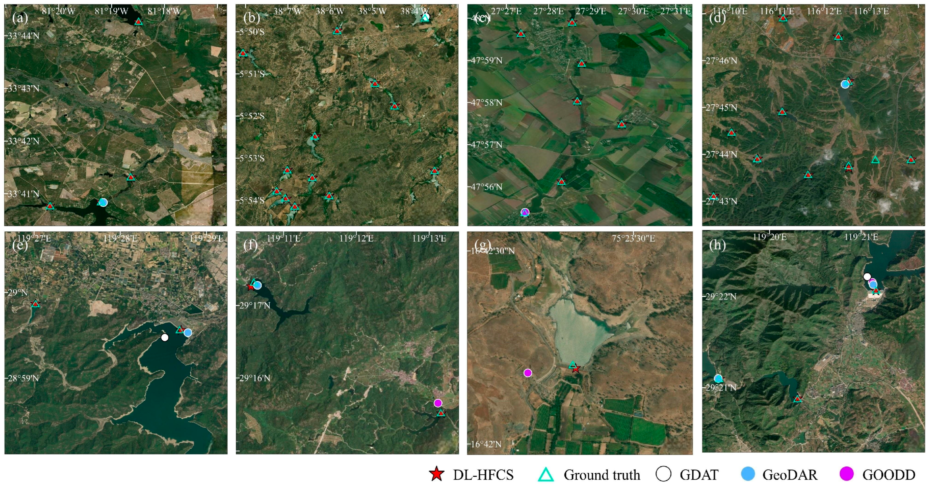
4.4. Comparison with Existing Global Dam Datasets

To comprehensively assess the reliability of DL-HFCS, we further compared the dam detection results of DL-HFCS and the global dam datasets (GeoDAR, GDAT, and GOODD) from quantity and positional deviation. In the 91 1° × 1° test areas, there are significant differences in the number of dams (with reservoir areas ≥ 0.05 km²) across different datasets (

Table 6. Comparison of positional deviation between DL-HFCS detection results and global dam datasets.

Dataset	Count	0 m (%)	(0, 50] m (%)	(50, 100] m (%)	>100 m (%)
GeoDAR	1043	69.42	15.92	6.62	8.05
GDAT	983	73.65	12.41	7.43	9.56
GOODD	926	58.53	12.53	10.37	18.57
DL-HFCS	9903	98.08	0.68	0.78	0.46

, Figure 10a–d). Specifically, GeoDAR contains 1043 dams, GDAT has 983 dams, GOODD includes 926 dams, and DL-HFCS detected 9903 dams. The total number of unique dams for these three datasets is 1923, of which DL-HFCS detected 1488 dams. In other words, DL-HFCS can supplement these three datasets with 8415 dams.

There are also significant differences in the positional deviation of dams across different datasets (Table 6, Figure 10e–h). For dams detected by DL-HFCS, 98% of their centroids are located within the annotated boxes in the prediction set. In contrast, this proportion is below 75% for the other three global dam datasets. When the positional deviation range is extended to 100 m, DL-HFCS performs best, achieving a proportion of 99.54%. This superior performance is primarily attributed to introducing the CIOU loss function during the training of YOLOv5s, which considers the overlapping area of the bounding boxes and incorporates measurements of the center point distance and aspect ratio, enabling precise localization of dams. For GeoDAR and GDAT, the proportion of dams with positional errors exceeding 100 m is within 10%, while GOODD has nearly 20%, significantly higher than DL-HFCS’s 0.46%.

5. Discussion

5.1. Impact of HFCS on Dam Detection Performance

We filtered dams in the prediction set based on the constraints in the HFCS and counted the number of dams that did not meet the constraints. In reservoirs with an area ≥ 1 km², there are 11 reservoirs where the distance between two dams within the reservoir is <500 m, whereas in reservoirs with an area < 1 km², 137 reservoirs contain two dams. According to the single reservoir-based dam number constraint, 148 dams in the prediction set could not be detected because they did not satisfy the condition.

Limited to accuracy in AW3D30, 880 dams could not be detected. Among these, 580 dams lacked river networks within the annotated boxes, 291 did not satisfy the constraint applicable to one branch, and 9 did not satisfy the constraint applicable to multi-branches. Notably, some dams in the prediction set simultaneously did not satisfy multiple constraints. Data cleaning was performed to avoid duplicate counting. Finally, 11,056 dams in the prediction set met all constraints, meaning a maximum recall of 91.84% under HFCS (

Table 7. The number of dams in the prediction set that meet different constraint conditions.

Constraints	Qualified	Unqualified	Proportion (%)
single reservoir-based dam number	11,890	148	98.77
watershed river network	11,458	580	95.18
elevation difference (multi-branches)	5638	9	99.84
elevation difference (one branch)	5520	291	94.99
All	11,056	982	91.84

).

Detection box-based river network elevation difference constraint is vital in HFCS. The basic idea is to reflect the elevation differences between up and downstream dams through ranked river networks and the Digital Surface Model (DSM). In the prediction set, only 580 dams did not intersect with river networks, while the remaining 11,458 included river networks. This result validates the rationality of the watershed river network constraint, as over 95% of dams satisfy this condition. Among the 5647 dams with multi- branches, 99.84% (5638) met the condition that the downstream water body ratio is smaller than the upstream water body ratio (Table 7); however, nine dams did not meet this condition (Figure 11).

Among the 5811 dams with one branch, 94.99% (5520) met the condition that the maximum elevation value of the water body part is higher than the median elevation value of the land part (Table 7). The remaining 291 dams have an inverse elevation difference between the water body and the land part in the range of [−25, 0) meters, with 95% of these within [−5, 0) meters. Considering that the overall vertical accuracy of AW3D30 is 5 m, there may be some uncertainty in the actual measured elevation differences between the water body and land parts. Thus, this error is considered acceptable. The remaining six dams with elevation differences < −10 m were all constructed within narrow valleys (Figure 12).

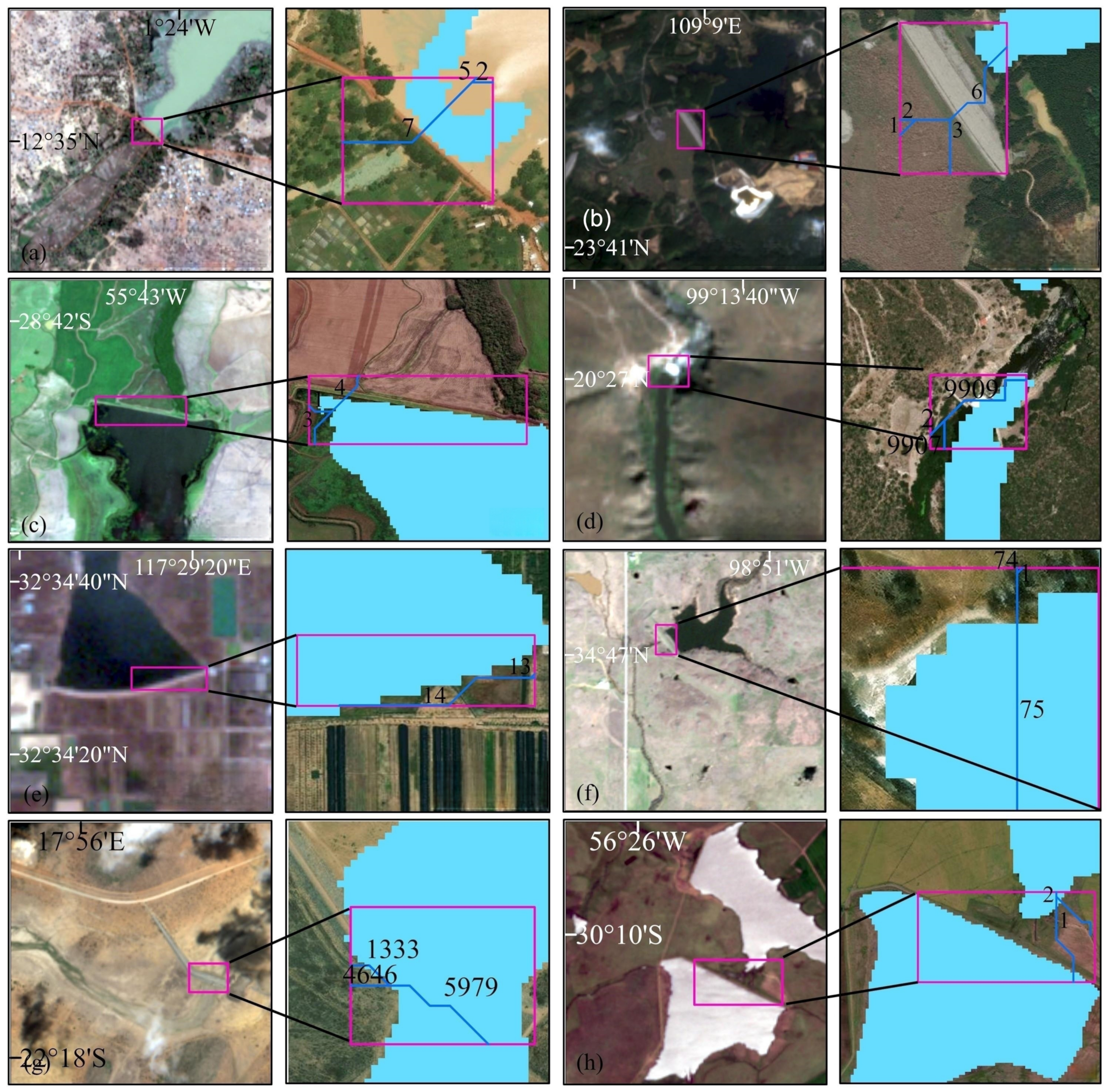
5.2. Analysis of False Detections

Under DL-HFCS, there are 1575 false detection boxes, with 694 boxes having multi- branches and 881 boxes having one branch. By visually inspecting these boxes using Google Earth high-resolution imagery, the features within the boxes were categorized into four types: water-based artificial structures such as bridges and rolled dams (144, accounting for 9.14%), natural riverbanks (309, accounting for 19.62%), coastal areas (49, accounting for 3.11%), and land-based artificial structures such as roads or ponds (1073, accounting for 68.13%) (Figure 13).

Compared to high-resolution remote sensing imagery, the proportion of false detection features in medium resolution differs. In Sentinel-2 imagery, roads and riverbanks are challenging to distinguish, especially bridges, and rolled dams are often mistakenly identified as dams. These features appear as white linear features in Sentinel-2 imagery and satisfy the elevation difference constraint, making them hard to eliminate accurately. However, in high-resolution imagery, these false detection objects have apparent geometric differences from dams, allowing them to be easily distinguished. Additionally, natural riverbanks near water bodies should theoretically be eliminated through the elevation difference constraint. However, due to the precision limitations of AW3D30 data, they are difficult to eliminate effectively.

5.3. Strengths and Limitations of DL-HFCS

The experiment successfully detected 9903 dams within 91 global test areas using DL-HFCS. Compared to only the YOLOv5s model, introducing HFCS improved the precision by approximately 47.58%, reaching 86.29%. This study conducted an in-depth analysis of the hydrological features of dams, utilizing river network and elevation data to reduce false alarms. In contrast, existing research focuses on terrain-sensitive indices such as undulation and roughness and relies on empirical thresholds for judgment, lacking specific analysis for site selection.

Furthermore, for cases with one branch where determining elevation differences is challenging, the constraint was inspired by DDRM. The elevation distribution of water and land parts within dam detection boxes was calculated for comparative analysis. However, for dams where the upstream and downstream water body areas are similar, DDRM may mistakenly delete the dams [30], whereas this method accurately distinguishes and retains these dams.

Nevertheless, there are still some limitations. In the prediction set, all dams meet the reservoir area ≥ 0.05 km². However, reservoir areas vary with seasonal changes [55]. When water body data cannot accurately reflect the annual distribution of reservoir areas, some qualified dams may be excluded from the prediction set. The ESRI water body product faces the same issue. Future research will overcome this by comparing the accuracy of different water body products and combining them to obtain stable water body areas.

Regarding DSM data, the AW3D30 used differs from the Sentinel-2 imagery detection year by approximately ten years. Dams constructed during this period may fail to meet the elevation difference constraint due to the DSM data not being updated on time. Additionally, the vertical error of AW3D30 is significantly influenced by slope; in areas with slopes < 20°, the vertical error is minimal [48,49]. However, dams are often built in hilly or mountainous regions with steeper slopes. These areas exhibit pronounced undulation and varying surface features, such as trees and rocks, further affecting the vertical error. Future studies should consider combining DSM and DTM data and selecting products with closer acquisition years and higher spatial resolutions, especially in high-slope areas, to reduce vertical errors and improve dam detection accuracy.

6. Conclusions

This study proposed a DL-HFCS dam detection method based on RGB and SNR samples from Sentinel-2 MSI remote sensing imagery. Applied to 91 global 1° × 1° test areas, it achieved a precision of 86.29% and a recall of 82.26%, enabling comprehensive and precise dam detection worldwide. DL-HFCS consists of two parts: DL for detecting dams in Sentinel-2 imagery and HFCS for eliminating false detection boxes. In the DL component, considering the reflectance characteristics of dams and water bodies across different bands, dam sample datasets (RGB) and dam sample datasets (SNR) were constructed to train the YOLOv5s (RGB) and YOLOv5s (SNR) models, respectively. Combining the detection results of both models can reduce the miss rate. In HFCS, a sequence of constraints—adjacent water constraint, single reservoir-based dam number constraint, watershed river network constraint, and detection box-based river network elevation difference constraint—eliminated the vast majority of false detection boxes, such as those caused by houses, shadows, white clouds, and snow. Due to the limitations in the water body and DSM data accuracy, some dams were inevitably mistakenly discarded during the constraint process.

In future studies, we plan to apply this method to Sentinel-2 MSI remote sensing imagery globally to develop a comprehensive and precise global dam dataset.

References

1. Zarfl, C.; Lumsdon, A.E.; Berlekamp, J.; Tydecks, L.; Tockner, K. A Global Boom in Hydropower Dam Construction. Aquat. Sci. 2015, 77, 161–170. [Google Scholar]
2. Grill, G.; Lehner, B.; Thieme, M.; Geenen, B.; Tickner, D.; Antonelli, F.; Babu, S.; Borrelli, P.; Cheng, L.; Crochetiere, H.; et al. Mapping the World’s Free-Flowing Rivers. Nature 2019, 569, 215–221. [Google Scholar] [CrossRef] [PubMed]
3. Belletti, B.; Garcia de Leaniz, C.; Jones, J.; Bizzi, S.; Börger, L.; Segura, G.; Castelletti, A.; van de Bund, W.; Aarestrup, K.; Barry, J.; et al. More than One Million Barriers Fragment Europe’s Rivers. Nature 2020, 588, 436–441. [Google Scholar] [PubMed]
4. Boulange, J.; Hanasaki, N.; Yamazaki, D.; Pokhrel, Y. Role of Dams in Reducing Global Flood Exposure under Climate Change. Nat. Commun. 2021, 12, 417. [Google Scholar]
5. Januchowski-Hartley, S.R.; McIntyre, P.B.; Diebel, M.; Doran, P.J.; Infante, D.M.; Joseph, C.; Allan, J.D. Restoring Aquatic Ecosystem Connectivity Requires Expanding Inventories of Both Dams and Road Crossings. Front. Ecol. Environ. 2013, 11, 211–217. [Google Scholar]
6. Mantel, S.K.; Rivers-Moore, N.; Ramulifho, P. Small Dams Need Consideration in Riverscape Conservation Assessments. Aquat. Conserv. Mar. Freshw. Ecosyst. 2017, 27, 748–754. [Google Scholar] [CrossRef]
7. Grinham, A.; Albert, S.; Deering, N.; Dunbabin, M.; Bastviken, D.; Sherman, B.; Lovelock, C.E.; Evans, C.D. The Importance of Small Artificial Water Bodies as Sources of Methane Emissions in Queensland, Australia. Hydrol. Earth Syst. Sci. 2018, 22, 5281–5298. [Google Scholar] [CrossRef]
8. Carolli, M.; Garcia de Leaniz, C.; Jones, J.; Belletti, B.; Huđek, H.; Pusch, M.; Pandakov, P.; Börger, L.; van de Bund, W. Impacts of Existing and Planned Hydropower Dams on River Fragmentation in the Balkan Region. Sci. Total Environ. 2023, 871, 161940. [Google Scholar] [CrossRef]
9. Lehner, B.; Beames, P.; Mulligan, M.; Zarfl, C.; De Felice, L.; van Soesbergen, A.; Thieme, M.; Garcia de Leaniz, C.; Anand, M.; Belletti, B.; et al. The Global Dam Watch Database of River Barrier and Reservoir Information for Large-Scale Applications. Sci. Data 2024, 11, 1069. [Google Scholar]
10. Cracknell, A.P. The Development of Remote Sensing in the Last 40 Years. Int. J. Remote Sens. 2018, 39, 8387–8427. [Google Scholar] [CrossRef]
11. Chang, L.; Cheng, L.; Chen, J.; Han, D.; Zhang, L.; Liu, P.; Chang, J. Comparison and Application of Georeferenced Reservoir and Dam Data Sets. China Rural Water Hydropower. 2023, 6, 1–11. [Google Scholar]
12. Zhang, Z.; Liu, Q.; Wang, Y. Road Extraction by Deep Residual U-Net. IEEE Geosci. Remote Sens. Lett. 2018, 15, 749–753. [Google Scholar]
13. Zuo, J.; Xu, G.; Fu, K.; Sun, X.; Sun, H. Aircraft Type Recognition Based on Segmentation with Deep Convolutional Neural Networks. IEEE Geosci. Remote Sens. Lett. 2018, 15, 282–286. [Google Scholar]
14. Bentes, C.; Velotto, D.; Tings, B. Ship Classification in TerraSAR-X Images With Convolutional Neural Networks. IEEE J. Ocean. Eng. 2018, 43, 258–266. [Google Scholar]
15. Audebert, N.; Le Saux, B.; Lefèvre, S. Beyond RGB: Very High Resolution Urban Remote Sensing with Multimodal Deep Networks. ISPRS J. Photogramm. Remote Sens. 2018, 140, 20–32. [Google Scholar]
16. Shen, Y.; Xu, S. Effective method for dam recognition from visible images. Comput. Appl. 2006, 08, 1972–1974. [Google Scholar]
17. Fang, W.; Sun, Y.; Ji, R.; Wan, W.; Ma, L. Recognizing Global Dams from High-Resolution Remotely Sensed Images Using Convolutional Neural Networks. IEEE J. Sel. Top. Appl. Earth Obs. Remote Sens. 2021, 14, 6363–6371. [Google Scholar] [CrossRef]
18. Lehner, B.; Liermann, C.R.; Revenga, C.; Vörösmarty, C.; Fekete, B.; Crouzet, P.; Döll, P.; Endejan, M.; Frenken, K.; Magome, J.; et al. High-resolution Mapping of the World’s Reservoirs and Dams for Sustainable River-flow Management. Front. Ecol. Environ. 2011, 9, 494–502. [Google Scholar]
19. Wang, J.; Walter, B.A.; Yao, F.; Song, C.; Ding, M.; Maroof, A.S.; Zhu, J.; Fan, C.; McAlister, J.M.; Sikder, S.; et al. GeoDAR: Georeferenced Global Dams and Reservoirs Dataset for Bridging Attributes and Geolocations. Earth Syst. Sci. Data 2022, 14, 1869–1899. [Google Scholar]
20. Mulligan, M.; Van Soesbergen, A.; Sáenz, L. GOODD, a Global Dataset of More than 38,000 Georeferenced Dams. Sci. Data 2020, 7, 31. [Google Scholar]
21. Zhang, A.T.; Gu, V.X. Global Dam Tracker: A Database of More than 35,000 Dams with Location, Catchment, and Attribute Information. Sci. Data 2023, 10, 111. [Google Scholar] [CrossRef] [PubMed]
22. Wang, X.; Xiao, X.; Qin, Y.; Dong, J.; Wu, J.; Li, B. Improved Maps of Surface Water Bodies, Large Dams, Reservoirs, and Lakes in China. Earth Syst. Sci. Data 2022, 14, 3757–3771. [Google Scholar] [CrossRef]
23. Paredes-Beltran, B.; Sordo-Ward, A.; Garrote, L. Dataset of Georeferenced Dams in South America (DDSA). Earth Syst. Sci. Data 2021, 13, 213–229. [Google Scholar] [CrossRef]
24. Speckhann, G.A.; Kreibich, H.; Merz, B. Inventory of Dams in Germany. Earth Syst. Sci. Data 2021, 13, 731–740. [Google Scholar] [CrossRef]
25. Song, C.; Fan, C.; Zhu, J.; Wang, J.; Sheng, Y.; Liu, K.; Chen, T.; Zhan, P.; Luo, S.; Yuan, C.; et al. A Comprehensive Geospatial Database of Nearly 100 000 Reservoirs in China. Earth Syst. Sci. Data 2022, 14, 4017–4034. [Google Scholar] [CrossRef]
26. Fan, C.; Song, C.; Wang, J.; Sheng, Y.; Lin, Y.; Yuan, C.; Safat Sikder, M.; Crétaux, J.-F.; Liu, K.; Chen, T.; et al. Emerging Global Reservoirs in the New Millennium: Abundance, Hotspots, and Total Water Storage. Sci. Bull. 2024, 69, 2179–2182. [Google Scholar] [CrossRef]
27. Mao, J.; Cheng, L.; Ji, C.; Jing, M.; Duan, Z.; Li, N.; Gesang, Z.; Li, M. Verification of Dam Spatial Location in Open Datasets Based on Geographic Knowledge and Deep Learning. IEEE J. Sel. Top. Appl. Earth Obs. Remote Sens. 2022, 15, 7277–7287. [Google Scholar] [CrossRef]
28. Jing, M.; Cheng, L.; Ji, C.; Mao, J.; Li, N.; Duan, Z.; Li, Z.; Li, M. Detecting Unknown Dams from High-Resolution Remote Sensing Images: A Deep Learning and Spatial Analysis Approach. Int. J. Appl. Earth Obs. Geoinformation 2021, 104, 102576. [Google Scholar] [CrossRef]
29. Jing, Y.; Ren, Y.; Liu, Y.; Wang, D.; Yu, L. Dam Extraction from High-Resolution Satellite Images Combined with Location Based on Deep Transfer Learning and Post-Segmentation with an Improved MBI. Remote Sens. 2022, 14, 4049. [Google Scholar] [CrossRef]
30. Wang, L.; Xu, Y.; Chen, Q.; Wu, J.; Luo, J.; Li, X.; Peng, R.; Li, J. Research on Remote-Sensing Identification Method of Typical Disaster-Bearing Body Based on Deep Learning and Spatial Constraint Strategy. Remote Sens. 2024, 16, 1161. [Google Scholar] [CrossRef]
31. Zhao, G.; Yao, P.; Fu, L.; Zhang, Z.; Lu, S.; Long, T. A Deep Learning Method Based on Two-Stage CNN Framework for Recognition of Chinese Reservoirs with Sentinel-2 Images. Water 2022, 14, 3755. [Google Scholar] [CrossRef]
32. Cao, Y.; Weng, Q. A Deep Learning-Based Super-Resolution Method for Building Height Estimation at 2.5 m Spatial Resolution in the Northern Hemisphere. Remote Sens. Environ. 2024, 310, 114241. [Google Scholar]
33. Zeng, F.; Cheng, L.; Li, N.; Xia, N.; Ma, L.; Zhou, X.; Li, M. A Hierarchical Airport Detection Method Using Spatial Analysis and Deep Learning. Remote Sens. 2019, 11, 2204. [Google Scholar] [CrossRef]
34. Li, N.; Cheng, L.; Huang, L.; Ji, C.; Jing, M.; Duan, Z.; Li, J.; Li, M. Framework for Unknown Airport Detection in Broad Areas Supported by Deep Learning and Geographic Analysis. IEEE J. Sel. Top. Appl. Earth Obs. Remote Sens. 2021, 14, 6328–6338. [Google Scholar]
35. Redmon, J.; Divvala, S.; Girshick, R.; Farhadi, A. You Only Look Once: Unified, Real-Time Object Detection. In Proceedings of the 2016 IEEE Conference on Computer Vision and Pattern Recognition (CVPR), Vegas, NV, USA, 27–30 June 2016; pp. 779–788. [Google Scholar]
36. Liu, W.; Anguelov, D.; Erhan, D.; Szegedy, C.; Reed, S.; Fu, C.-Y.; Berg, A.C. SSD: Single Shot MultiBox Detector. In Proceedings of the Computer Vision—ECCV 2016, Amsterdam, The Netherlands, 11–14 October 2016; pp. 21–37. [Google Scholar]
37. Ren, S.; He, K.; Girshick, R.; Sun, J. Faster R-CNN: Towards Real-Time Object Detection with Region Proposal Networks. IEEE Trans. Pattern Anal. Mach. Intell. 2017, 39, 1137–1149. [Google Scholar]
38. DETRs Beat YOLOs on Real-Time Object Detection|IEEE Conference Publication|IEEE Xplore. Available online: https://ieeexplore.ieee.org/document/10657220 (accessed on 4 March 2025).
39. Jocher, G.; Chaurasia, A.; Stoken, A.; Borovec, J.; NanoCode012; Kwon, Y.; Michael, K.; TaoXie; Fang, J.; imyhxy; et al. Ultralytics/Yolov5. Available online: https://github.com/ultralytics/yolov5 (accessed on 10 December 2024).
40. Wang, C.-Y.; Mark Liao, H.-Y.; Wu, Y.-H.; Chen, P.-Y.; Hsieh, J.-W.; Yeh, I.-H. CSPNet: A New Backbone That Can Enhance Learning Capability of CNN. In Proceedings of the 2020 IEEE/CVF Conference on Computer Vision and Pattern Recognition Workshops (CVPRW), Seattle, WA, USA, 14–19 June 2020; pp. 1571–1580. [Google Scholar]
41. Fang, W.; Wang, C.; Chen, X.; Wan, W.; Li, H.; Zhu, S.; Fang, Y.; Liu, B.; Hong, Y. Recognizing Global Reservoirs from Landsat 8 Images: A Deep Learning Approach. IEEE J. Sel. Top. Appl. Earth Obs. Remote Sens. 2019, 12, 3168–3177. [Google Scholar]
42. Chen, Q.; Mudd, S.M.; Attal, M.; Hancock, S. Extracting an Accurate River Network: Stream Burning Re-Revisited. Remote Sens. Environ. 2024, 312, 114333. [Google Scholar]
43. He, C.; Yang, C.-J.; Turowski, J.M.; Ott, R.F.; Braun, J.; Tang, H.; Ghantous, S.; Yuan, X.; Stucky de Quay, G. A Global Dataset of the Shape of Drainage Systems. Earth Syst. Sci. Data 2024, 16, 1151–1166. [Google Scholar]
44. Frantz, D.; Haß, E.; Uhl, A.; Stoffels, J.; Hill, J. Improvement of the Fmask Algorithm for Sentinel-2 Images: Separating Clouds from Bright Surfaces Based on Parallax Effects. Remote Sens. Environ. 2018, 215, 471–481. [Google Scholar]
45. Brown, C.F.; Brumby, S.P.; Guzder-Williams, B.; Birch, T.; Hyde, S.B.; Mazzariello, J.; Czerwinski, W.; Pasquarella, V.J.; Haertel, R.; Ilyushchenko, S.; et al. Dynamic World, Near Real-Time Global 10 m Land Use Land Cover Mapping. Sci. Data 2022, 9, 251. [Google Scholar]
46. Lesiv, M.; See, L.; Laso Bayas, J.C.; Sturn, T.; Schepaschenko, D.; Karner, M.; Moorthy, I.; McCallum, I.; Fritz, S. Characterizing the Spatial and Temporal Availability of Very High Resolution Satellite Imagery in Google Earth and Microsoft Bing Maps as a Source of Reference Data. Land 2018, 7, 118. [Google Scholar] [CrossRef]
47. Liang, J.; Gong, J.; Li, W. Applications and Impacts of Google Earth: A Decadal Review (2006–2016). ISPRS J. Photogramm. Remote Sens. 2018, 146, 91–107. [Google Scholar]
48. Tadono, T.; Nagai, H.; Ishida, H.; Oda, F.; Naito, S.; Minakawa, K.; Iwamoto, H. GENERATION OF THE 30 M-MESH GLOBAL DIGITAL SURFACE MODEL BY ALOS PRISM. Int. Arch. Photogramm. Remote Sens. Spat. Inf. Sci. 2016, XLI-B4, 157–162. [Google Scholar]
49. Takaku, J.; Tadono, T.; Tsutsui, K.; Ichikawa, M. VALIDATION OF “AW3D” GLOBAL DSM GENERATED FROM ALOS PRISM. ISPRS Ann. Photogramm. Remote Sens. Spat. Inf. Sci. 2016, III–4, 25–31. [Google Scholar]
50. Karra, K.; Kontgis, C.; Statman-Weil, Z.; Mazzariello, J.C.; Mathis, M.; Brumby, S.P. Global Land Use/Land Cover with Sentinel 2 and Deep Learning. In Proceedings of the 2021 IEEE International Geoscience and Remote Sensing Symposium IGARSS, Brussels, Belgium, 11–16 July 2021; pp. 4704–4707. [Google Scholar]
51. Venter, Z.S.; Barton, D.N.; Chakraborty, T.; Simensen, T.; Singh, G. Global 10 m Land Use Land Cover Datasets: A Comparison of Dynamic World, World Cover and Esri Land Cover. Remote Sens. 2022, 14, 4101. [Google Scholar] [CrossRef]
52. Xia, G.-S.; Bai, X.; Ding, J.; Zhu, Z.; Belongie, S.; Luo, J.; Datcu, M.; Pelillo, M.; Zhang, L. DOTA: A Large-Scale Dataset for Object Detection in Aerial Images. In Proceedings of the 2018 IEEE/CVF Conference on Computer Vision and Pattern Recognition (CVPR), Salt Lake City, UT, USA, 18–22 June 2018; pp. 3974–3983. [Google Scholar]
53. Li, K.; Wan, G.; Cheng, G.; Meng, L.; Han, J. Object Detection in Optical Remote Sensing Images: A Survey and a New Benchmark. ISPRS J. Photogramm. Remote Sens. 2020, 159, 296–307. [Google Scholar]
54. Chen, Y.; Wang, B.; Guo, X.; Zhu, W.; He, J.; Liu, X.; Yuan, J. DEYOLO: Dual-Feature-Enhancement YOLO for Cross-Modality Object Detection. In Proceedings of the Pattern Recognition—ICPR 2024, Kolkata, India, 1–5 December 2024; pp. 236–252. [Google Scholar]
55. Geraldes, A.M.; Boavida, M.-J. Seasonal Water Level Fluctuations: Implications for Reservoir Limnology and Management. Lakes Reserv. Sci. Policy Manag. Sustain. Use 2005, 10, 59–69. [Google Scholar] [CrossRef]
Figure 1. Band selection and model training process.
Remotesensing 17 01194 g001
Figure 2. Schematic of dam detection based on deep learning models.
Remotesensing 17 01194 g002
Figure 3. An example of adjacent water body constraint after deep learning. (The red box is the detection box of YOLOv5s (RGB), the yellow box is the detection box of YOLOv5s (SNR)).
Remotesensing 17 01194 g003
Figure 4. An example of single reservoir-based dam number constraint. (a) For small reservoirs (<C km2), only dam1st (0.851) is retained; (b) For larger reservoirs (≥C km2), only dam1st (0.923) is retained, while dam2nd (0.916) is discarded due to its distance from dam1st less than D m. (b1b3 are the locations detected by the models as dams).
Remotesensing 17 01194 g004
Figure 5. An example of watershed river network constraint (Image Source: Sentinel-2/Google Earth). ((ad) Steps to generate river networks; (eg) There are two river networks with different numbers of branches in the detection box. One network has five branches, while the other has just one. The river network with five branches is retained; (hj) There are two river networks with the same number of branches in the detection box. The first has a total branch length of 165 m, and the second has 188 m. The river network with the longer length is retained). (The red box is the buffered detection box of YOLOv5s (RGB) or YOLOv5s (SNR)).
Remotesensing 17 01194 g005
Figure 6. An example of detection box-based river network elevation difference constraint (Image Source: Sentinel-2/Google Earth). (a) For river networks with multi-branches, the total water–body intersection ratio of the upstream branch set is greater than or equal to that in the downstream branch, the detection box is retained; (b) For river networks with only one branch, max(Hwater) (113 m) exceeds median(Hland) (108 m), water flows toward the land part, the detection box is retained. (The red box is the buffered detection box of YOLOv5s (RGB) or YOLOv5s (SNR)).
Remotesensing 17 01194 g006
Figure 7. Test areas in global experiments for DL-HFCS.
Remotesensing 17 01194 g007
Figure 8. Spatial distribution of dam sample points and examples of dam samples in different Sentinel-2 band combinations. (a) The Spatial distribution of dam sample points; (bd) The dam annotation box in RGB band combination; (eg) The dam annotation box in SNR band combination. (The red box is the annotation box).
Remotesensing 17 01194 g008
Figure 9. Validation accuracy of YOLOv5s (RGB) and YOLOv5s (SNR) models in the training process. (a) Precision and recall curves during the training process of YOLOv5S (RGB) model; (b) Precision and recall curves during the training process of YOLOv5S (SNR) model.
Remotesensing 17 01194 g009
Figure 10. Comparison of DL-HFCS detection results with global dam datasets (Image Source: Google Earth). ((ad) Comparison in terms of quantity; (eh) Comparison in terms of positional deviation).
Remotesensing 17 01194 g010
Figure 11. Examples of dam bounding boxes in the prediction set that do not meet the elevation difference constraint under multi-branches (Image Source: Sentinel-2/Google Earth) ((a,b) are located in Katenga, Burkina Faso, and Laibin City, China. Both experienced severe droughts in 2021, leading to most reservoirs being in a desiccated state; (c) shows water bodies of reservoirs covered by dense aquatic vegetation that failed to be identified; (dh) illustrate that the generated river network has directional discrepancies in river flow). (The purple box is the annotation box).
Remotesensing 17 01194 g011
Figure 12. Examples of dam annotated boxes in the prediction set that do not meet the elevation difference constraint under one branch (Image Source: Sentinel-2). (a) Dam annotated box does not meet the constraint; (b) The elevation histogram of annotated box in a; (c) Dam annotated box does not meet the constraint; (d) The elevation histogram of annotated box in c. (Purple represents the water part, and brown represents the land part).
Remotesensing 17 01194 g012
Figure 13. Examples of false detection boxes (the first column is Sentinel-2 RGB bands, the second is Sentinel-2 SNR bands, and the third is Google Earth high-resolution images) ((ac) water-based artificial structure; (df) natural riverbank; (gi) natural riverbank; (jl) land-based artificial structures). (The red box is the buffered detection box of YOLOv5s (RGB) or YOLOv5s (SNR)).
Remotesensing 17 01194 g013