Highlights
What are the main findings?
- We propose a normalized metric (TDM) that effectively integrates contrast (), variance (), and Jensen–Shannon Divergence () into a unified quantitative indicator.
- We combine the analysis of this proposed metric with quality assessment through a novel approach using Image Horizontal Visibility Graphs (IHVG) based on ratio images.
What are the implication of the main findings?
- The proposed approach discriminates between filters that only suppress variance and those that effectively restore the statistical randomness of the ratio images.
- The proposed quality assessment framework enables the integrated evaluation of image quality by combining statistical descriptors with graph-based texture analysis, providing a more comprehensive characterization of despeckling performance.
Abstract
We present a quantitative and qualitative evaluation of despeckling filters based on a set of Haralick-derived features and the Jensen–Shannon Divergence obtained from ratio images. To that aim, we propose a normalized composite index, called the Texture-Divergence Measurement (), that describes the statistical and structural behavior of the filtered images. Complementary qualitative analysis using Image Horizontal Visibility Graphs (IHVGs) confirms the results of the proposed metric. The combination of the proposed metric and IHVG visualization provides a robust framework for assessing despeckling performance from both statistical and structural perspectives.
1. Introduction
Synthetic Aperture Radar (SAR) is an advanced remote sensing technology that relies on active microwave sensors to acquire high-resolution information from the Earth’s surface. Unlike passive optical systems, SAR transmits microwave signals toward the target scene and records the amplitude and phase of the backscattered echoes to reconstruct two-dimensional images of the terrain [1]. This capability allows SAR systems to operate independently of solar illumination and under virtually all weather conditions, making them invaluable for applications in environmental monitoring, disaster management, agriculture, hydrology, and urban studies.
However, despite its advantages, SAR imagery is inherently degraded by a granular interference pattern known as speckle [2]. Speckle arises from the coherent nature of radar imaging, where the constructive and destructive interference of backscattered signals within a resolution cell produces noise-like fluctuations. While speckle preserves the radiometric properties of the scattering medium, it significantly reduces the visual quality of the images and complicates subsequent processing tasks such as classification, segmentation, target detection, and change detection. Therefore despeckling has been recognized as a critical preprocessing step in the SAR image analysis pipeline.
Research on despeckling has been highly active for several decades, leading to the development of a wide spectrum of methodologies that can be broadly categorized according to the underlying principles they employ. Classical local filtering approaches, such as the Lee filter [3], rely on the statistical properties of spatially adjacent pixels to estimate the true reflectivity, thus attenuating noise while attempting to preserve local structures and edges. While computationally efficient, these methods often suffer from excessive smoothing or detail loss in highly textured or heterogeneous areas.
To address these limitations, non-local filtering techniques have emerged, which exploit the redundancy of similar patches across the image rather than limiting the analysis to local neighborhoods [4]. These methods, inspired by the non-local means paradigm, have demonstrated superior performance in balancing noise suppression and structural preservation, especially in complex scenes.
More recently, the field has had a rapid shift toward data-driven and learning-based approaches. In particular, machine and deep learning methods have been increasingly applied to despeckling tasks [5,6,7,8]. Convolutional neural networks (CNNs) [9,10,11,12,13,14,15] and transformer-based models [12,16,17,18,19] are capable of learning complex mappings between noisy and clean representations, often outperforming traditional model-based filters in terms of both quantitative metrics and perceptual quality. These methods benefit from large annotated datasets and the ability to generalize across diverse imaging conditions, although they introduce challenges related to training data requirements, interpretability, and computational cost.
The evaluation of despeckling algorithms constitutes an ongoing and dynamic area of research within the field of SAR image processing. A rigorous assessment of the quality of despeckling is essential to determine the effectiveness of filtering techniques and to quantify their impact on fundamental image characteristics. In particular, the evaluation process must simultaneously address two critical and often competing objectives: the suppression of speckle noise, which enhances image interpretability, and the preservation of structural details such as edges and fine textures.
To achieve this, a variety of quantitative performance metrics have been developed and widely adopted in the SAR community. Among the most frequently employed are the Equivalent Number of Looks (ENL), which provides an estimation of noise reduction; the Mean Squared Error (MSE), which quantifies pixel-level discrepancies between the despeckled image and a reference; and the Structural Similarity Index (SSIM), which evaluates perceived similarity by incorporating reflectivity, contrast, and structural information. In addition, edge-preservation capabilities are often assessed through Pratt’s Figure of Merit (PFOM), which specifically measures the accuracy of edge localization after filtering.
Beyond these classical measures, recent research has also explored approaches for despeckling quality assessment grounded on the statistical properties of SAR imagery. One such approach is the analysis of ratio images, which involves examining the statistical properties of the ratio between the observed SAR image and the despeckled result.
A perfect despeckling filter would produce a ratio image comprised of independent identically distributed samples from the Gamma distribution with unitary mean and scale equal to the number of looks. By examining how the observed ratio image deviates from this ideal situation, one can evaluate the properties of the filter.
This methodology has proven particularly useful for capturing subtle variations in noise patterns and structural distortions that conventional indicators may overlook. Several studies, such as those presented in Refs. [20,21,22,23], have highlighted the potential of ratio-image-based metrics to complement traditional evaluation criteria, thereby contributing to a more comprehensive and robust framework for assessing despeckling performance.
We deepen the analysis of the ratio images, including the degree of the visibility graphs, Haralick feature extraction, and divergence to evaluate their remaining structure. The inclusion of visibility graphs is particularly relevant, as their degree statistics provide a sensitive indicator of residual spatial organization: deviations from the expected patterns of fully developed speckle become apparent through shifts in node connectivity, alterations in scale-free behavior, or changes in local structural motifs. This graph-based perspective complements traditional second-order statistics, enabling a more discriminative assessment of the underlying texture persistence in the filtered outputs. We showcase that this approach is effective in assessing the filters analyzed by Gómez et al. [23].
A key limitation in ratio-image–based despeckling assessment is the underlying assumption that speckle strictly follows a gamma distribution associated with fully developed speckle. In practice, deviations from this model may arise due to scene heterogeneity, anisotropic scattering, or changes in image resolution that alter the underlying speckle statistics. These factors can reduce the reliability of statistical evaluations, including divergence measures such as the Jason–Shannon divergence, which presuppose ideal noise behavior. Consequently, the interpretability and robustness of ratio-image analyses may be compromised when these conditions are not fully satisfied. The physics of coherent imaging implies that, under the conditions described in Yue et al. [24], fully developed speckle follows a gamma distribution. This setting is naturally expressed through the multiplicative model, which provides a non-additive description of the data. When speckle is not fully developed, the multiplicative model can still be used to separate the observations into backscatter (X) and speckle (N); while the resulting measurements no longer follow a gamma distribution, speckle is still gamma-distributed.
2. Materials and Methods
2.1. SAR and Ratio Images
Under the widely accepted multiplicative model (for details, see Ref. [25]), a speckled image is the product of two independent random fields: X describes the backscatter, and Y the speckle:
The physics of coherent imaging leads to the gamma model with unitary mean for Y, characterized by the probability density function:
where L is the Equivalent Number of Looks (ENL) and is the gamma function [25]. We denote this situation as .
Moreover, speckle is a collection of independent identically distributed (iid) random variables. The model assumed for X completely characterizes the distribution of the return Y [24].
Despeckling filters aim at combating speckle. Thus, they produce an estimate of the backscatter . Ideally, this estimate coincides with the unobserved backscatter, i.e., the perfect filter is . In this ideal situation, the ratio of the image Y and the filtered image is pure speckle: . Deviations from the iid gamma model (2) characterize departures from the ideal filter.
Checking adherence to the gamma model is easier than verifying the independence hypothesis. Gómez et al. [22] used Haralik’s features and a permutation strategy to quantify departures from independence, while Vitale et al. [26] analyzed covariance matrices. Gomez et al. [27] proposed the -metric based on the closeness of the ratio image to the iid hypothesis. The perfect despeckling filter will produce , and the larger is, the further the filter is from the ideal. It is calculated according to Equation (3).
where is the absolute value of the relative residual due to deviations from the ideal ENL, and is the absolute value of the relative variation, combining the measures of the remaining structure and of deviations from the statistical properties of the ratio image.
2.2. Visibility Graphs
The concept of visibility graphs was originally introduced by Lacasa et al. [28] as a computationally efficient methodology for transforming time series into complex networks. In this framework, each observation of the time series is mapped to a node in the graph, while the connectivity between nodes is established according to a well-defined visibility criterion. This transformation allows time series to be studied using the tools of graph theory and complex network analysis, providing insights into structural properties, scaling behaviors, and dynamical patterns that are not easily captured by conventional statistical methods.
Building on this idea, in the present work we propose a novel visibility criterion grounded in the convexity of data pairs. Specifically, let us consider a time series , where is the temporal index and the corresponding observed value. Two arbitrary data points, and , are said to exhibit convex visibility, and therefore are represented as two connected nodes in the resulting graph, if, for every intermediate data point such that , the following convexity condition holds:
In other words, the value at any intermediate instant must lie strictly below the linear interpolation between and . Geometrically, this condition ensures that the straight line segment connecting and is not intersected by any intermediate data point. Thus, convex visibility preserves the intuitive notion of line-of-sight between observations, while incorporating a stricter criterion that highlights convex structural relationships within the time series. Equivalently, the nodes from observations and are horizontally connected if
By employing this convexity-based visibility criterion, the resulting graphs emphasize the geometric and structural properties inherent in the temporal evolution of the data. This approach is expected to enhance the ability to capture nonlinear dynamics, uncover hidden symmetries, and distinguish between different types of stochastic and deterministic processes.
Luque et al. [29] introduced the concept of Horizontal Visibility Graphs (HVG) as a computationally efficient alternative to the earlier Natural Visibility Graphs (NVG) proposed by Lacasa et al. [28]. While NVGs rely on a general geometric visibility criterion that requires verifying convexity relationships between pairs of data points, HVGs simplify this rule by restricting visibility to a horizontal condition, thereby reducing computational complexity and facilitating large-scale applications. Despite this simplification, HVGs have been shown to preserve many of the essential structural and statistical properties captured by NVGs, making them particularly attractive for the analysis of long time series.
Both NVG and HVG frameworks are designed to transform a one-dimensional sequence of measurements into a graph, where each observation in the time series is represented as a node. The edges in the graph are determined by the respective visibility criteria: in NVGs, two data points share an edge if the straight line segment connecting them does not intersect any intermediate observation, whereas in HVGs, visibility is restricted to whether intermediate values remain strictly below the minimum of the two endpoints.
Once the graph has been constructed, one of the fundamental descriptors used to characterize its topology is the degree of a node, defined as the number of connections (edges) it has with other nodes in the graph. The degree distribution, in particular, provides valuable information about the underlying dynamics of the time series. For example, it has been demonstrated that degree distributions extracted from visibility graphs can distinguish between stochastic processes, chaotic dynamics, and correlated noise, thereby serving as a bridge between nonlinear time series analysis and complex network theory.
Iacovacci and Lacasa [30] introduced the concepts of VG and HVG to IVG and HIVG, respectively, extending the visibility graph framework from one-dimensional time series to two-dimensional image data. In this approach, each pixel of the image is mapped to a node, and the visibility relationships between pixels are established according to geometric criteria adapted from the original visibility graph formalism. The same descriptors can be used once the graph is built. By computing the degree over local neighborhoods using a sliding window of size k, the authors proposed a reconstruction strategy that generates a new image representation—termed the k-image. This reconstructed k-image captures structural and spatial patterns embedded in the original data while filtering out redundant or less informative components.
In the present work, we propose using the k-image as an effective tool to evaluate the quality of despeckling algorithms in SAR imagery. Specifically, we argue that the degree-based reconstruction encapsulated in the k-image provides a meaningful quantification of structural information that persists after filtering. By varying the kernel size k, it becomes possible to adjust the sensitivity of the method: smaller values of k emphasize fine-grained local patterns, while larger values capture broader structural correlations.
This flexibility is particularly advantageous for the analysis of ratio images. Ratio images are expected to exhibit properties close to pure noise if the despeckling algorithm has successfully removed speckle without distorting the underlying structural information. By applying the IVG framework to ratio images and reconstructing k-images from node degree distributions, our methodology enables the visualization and quantification of residual structures that may indicate over-smoothing or incomplete noise suppression. Consequently, the proposed approach provides a novel and complementary perspective for assessing despeckling quality, bridging complex network theory and SAR image processing.
2.3. Haralick Features
Haralick features, first introduced by Haralick et al. [31], are a set of descriptors derived from Gray-Level Co-occurrence Matrices (GLCM). These matrices quantify how often pairs of pixel intensities occur in a given spatial relationship within an image. The GLCM captures second-order texture information by measuring the joint probability distribution of gray-level values at specified distances and orientations. From this matrix, Haralick proposed a collection of features that characterize different aspects of texture, such as uniformity, randomness, contrast, and correlation. These features include, among others, energy, entropy, contrast, correlation, homogeneity, and dissimilarity, each of which provides complementary insights into the spatial arrangement and distribution of pixel intensities.
Due to their ability to quantify textural patterns, Haralick features have been widely adopted in image analysis tasks across diverse domains, including medical imaging [32,33,34,35], remote sensing [36,37,38,39], and industrial inspection [40,41,42,43]. The robustness of these features arises from their mathematical formulation, which encapsulates texture properties in a compact quantitative representation while maintaining sensitivity to variations in image structure.
We will provide a rigorous, step-by-step presentation of Haralick texture descriptors calculated from the Gray Level Co-occurrence Matrix (GLCM). The presentation expands on the equations, taking into account numerical stability, and provides algorithmic steps for calculating each descriptor in the proposed analysis.
2.3.1. Notation and Discrete Geometry
Let denote a discrete gray-scale image defined on integer pixel coordinates . The image intensities are quantized to discrete gray levels:
A spatial offset (direction) is defined by a pair of integer displacements . For a displacement corresponding to a distance d and angle , in practice we use Equation (6):
and only pixel pairs that remain inside the image domain are used. Common directions are .
2.3.2. Definition of the (Un-Normalized) GLCM
For a fixed offset we define the (un-normalized) co-occurrence matrix P of size by counting occurrences:
This counts ordered pairs where the first pixel has intensity i and its neighbor at the given offset has intensity j.
Asymmetric GLCM uses as in Equation (7), while symmetric GLCM is obtained as . This makes the matrix symmetric and treats the pair as unordered. Either choice is valid but must be consistent across descriptors.
The counts are converted to probabilities by normalizing defined in the Equation (8):
where denotes the normalized co-occurrence probabilities for a given offset.
2.3.3. Auxiliary Marginal and Aggregated Distributions
2.3.4. Contrast
The contrast descriptor, also known as inertia or local variance, quantifies the intensity difference between a pixel and its neighbor over the entire image. It measures the degree of local variation present in the texture and is defined as Equation (13):
where denotes the number of quantized gray levels in the image, represents the normalized element of the GLCM, which expresses the joint probability of two pixels with gray levels i and j being spatially adjacent, and measures the squared intensity difference between the pair of gray levels.
High contrast values correspond to images with pronounced gray-level differences, indicating coarse or edge-rich textures. Conversely, low values represent smooth textures where neighboring pixels have similar gray levels.
2.3.5. Variance
The variance descriptor is defined as Equation (14):
where represents the mean gray level, given by Equation (15):
The Variance descriptor quantifies the dispersion of gray levels around the mean value , weighted by their marginal probabilities. It reflects the degree of heterogeneity in the texture. Higher variance indicates a broader distribution of intensity values (heterogeneous texture), while lower variance describes a more homogeneous or uniform region.
Unlike the contrast descriptor, which evaluates intensity differences between pixel pairs , the Variance focuses solely on the deviation of gray levels from their mean. This descriptor has the following properties:
- Non-negativity (),
- The minimum value min Variance = 0 is achieved when all pixels have the same gray level (),
- The maximum value occurs when the probability mass is evenly distributed at the two extremes max .
The Haralick descriptors provide complementary statistical summaries of texture patterns. Correct implementation requires careful handling of indexing, normalization, and numerical stability (especially for underflow). The step-by-step derivations and practical tips provided here are intended to make implementations reproducible and robust.
By extracting features such as contrast, entropy, correlation, and homogeneity, we are able to assess the extent to which despeckling algorithms succeed in removing speckle while avoiding the preservation or introduction of artificial structures. This approach thus provides a rigorous and complementary framework for evaluating despeckling quality, enhancing conventional statistical measures by incorporating second-order texture information. A comparison of the Haralick features of a pure noisy image with respect to the ratio of filtered images is part of the analysis proposed in this study.
2.4. Divergence Analysis
In a ratio image R, regions that are considered to be homogeneous are theoretically expected to follow a gamma probability distribution, which serves as the underlying statistical model for such areas. This expected distribution can then be contrasted with the analytical gamma distribution that characterizes the ideal statistical behavior of homogeneous regions in despeckled SAR images. Based on this, the degree of divergence between the empirical distribution derived from the ratio image and the analytical gamma distribution can be used as a quantitative measure to assess the effectiveness of the despeckling process. In other words, the closer the empirical distribution is to the theoretical gamma distribution, the higher the quality of the despeckling procedure is assumed to be.
To operationalize this comparison, we use the Jensen–Shannon Divergence (JSD), a symmetrized and smoothed version of the Kullback–Leibler divergence. The JSD is particularly advantageous in this context because it not only measures the dissimilarity between two probability distributions in a bounded and symmetric manner, but also ensures stability when handling finite samples. Consequently, it provides a robust statistical metric to evaluate the similarity between the observed and the analytical gamma distributions, and thereby serves as an informative indicator of despeckling performance [44,45]. The JSD is calculated according to Equation (17):
where is the Shanon entropy.
The divergence is obtained by estimating the Shannon entropy of both distributions, which requires discretizing the ratio image into a histogram and computing the corresponding probability mass function. These entropy values are then combined to measure how much the empirical distribution departs from the theoretical reference.
In the ideal scenario where the empirical distribution obtained from the homogeneous region of the ratio image perfectly matches the analytical gamma distribution, the JSD assumes a value of zero, indicating complete similarity between the two distributions. Conversely, any deviation from this ideal case, manifested as disparities between the empirical and theoretical distributions, results in progressively higher values of the JSD. Thus, the magnitude of the JSD can be interpreted as a direct indicator of the degree of mismatch between the distributions, and consequently, as a measure of the residual speckle or structural artifacts introduced during the despeckling process.
In addition to this divergence-based analysis, visual and statistical inspections of the ratio images provide complementary insights into despeckling quality. Specifically, first-order statistics—such as mean and variance—allow for the evaluation of marginal properties, ensuring that the despeckled image preserves the expected radiometric behavior in homogeneous regions. On the other hand, second-order statistics, which capture spatial dependencies through measures such as autocorrelation or gray-level co-occurrence matrices, are particularly useful in verifying the absence of structured patterns or textural remnants that may have been inadvertently introduced by the despeckling algorithm. By jointly examining both first- and second-order statistics alongside the JSD, a more comprehensive and reliable assessment of despeckling performance is achieved, bridging quantitative divergence measures with qualitative structural evaluations [23,27].
3. Experimental Results
Five SAR images in Single Look Complex (SLC) format of size 512 pixels × 512 pixels were selected from the region of Toronto, Ontario, Canada, as developed in [23].
3.1. Despeckled Images
These five samples were filtered with despeckling models documented in the literature such as: Autoencoder (AE) [7], FANS [4], Monet [46], and SCUNet [8]. The SAR and despeckled images are shown in Figure 1.
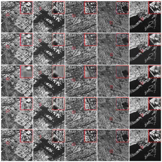
Figure 1.
SAR and filtered images. From top to bottom: SAR (SLC level), Filtered with AE, FANS, Monet, and SCUNet. Zoom of regions of interest in the red bounding boxes.
3.2. Ratio Images
Their respective ratio images are shown in Figure 2. These images have an average value of , calculated in a homogeneous area. This value of ENL which is used to obtain a pure gamma simulated image, as shown in Figure 3. This image is used for comparative purposes, since all the ratio images should resemble in the gamma distribution to this reference image.
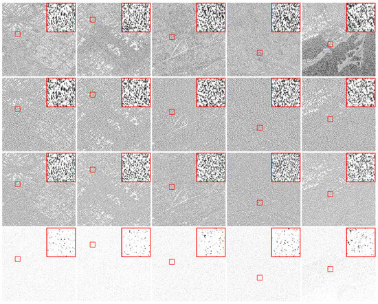
Figure 2.
Ratio images. From top to bottom: Filtered with AE, FANS, Monet, and SCUNet. Zoom of regions of interest in the red bounding boxes.
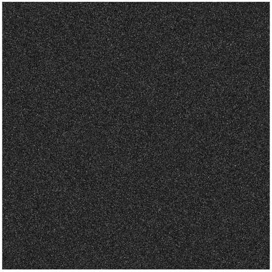
Figure 3.
Gamma generated sample with .
3.3. Haralick Features of Ratio Images and Gamma Samples
First, fourteen Haralick features were obtained from all the five samples despeckled with five filters. Also, the same features of the pure gamma images was obtained. These results are shown in Figure 4.
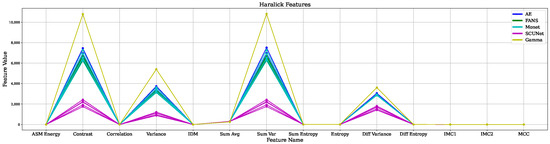
Figure 4.
Values of all 14 Haralick features of the ratio images.
The correlation matrix of these feautures obtained from all samples is shown in Figure 5. Also, several features have the same value, or even zero, in all samples. Based on this result, we decided to use only variance and contrast. Graphically, these two features for all the ratio images and gamma are shown in Figure 6, and a dispersion and histogram analysis in Figure 7.
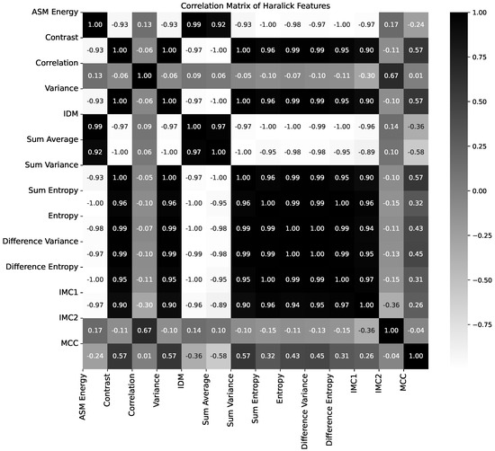
Figure 5.
Correlation matrix of all the 14 Haralick features of ratio images.
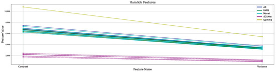
Figure 6.
Values of the 2 selected Haralick features of the ratio images.
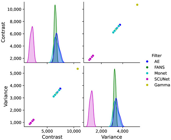
Figure 7.
Correlation analysis of selected Haralick features for despeckling filters and gamma distribution.
3.4. Divergence Analysis
Gamma models were estimated over a homogeneous region extracted from both the ratio image and the reference gamma-distributed image, as illustrated in Figure 8a. This estimation is used to model the statistical behavior of the pixel intensities under the assumption that the selected region represents an area with minimal spatial variability, thus allowing a reliable estimation of the underlying distribution parameters. The use of the gamma model is particularly appropriate for this type of imagery, as it provides an effective representation of multiplicative noise processes, such as the speckle in SAR imagery. Conversely, the histograms of the regions of interest in Figure 8b show a clear clustering of the plotted curves, indicating a consistent representation of the underlying data, particularly for the FANS, Monet, and gamma images.
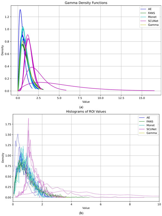
Figure 8.
Distribution analysis of filtered data. (a) Gamma probability density function fitting. (b) Histograms of regions of interest.
To complement this statistical modeling, a detailed texture analysis was performed based on the Haralick features. The resulting values of the Haralick features, together with the corresponding JSD metrics, are summarized in Table 1.

Table 1.
Measurement of , , , and -estimator of different despeckling filters and the gamma reference image.
The inclusion of the JSD provides a robust measure of the difference between the empirical distributions of the ratio image and the theoretical gamma model, thereby quantifying the degree of similarity between them. Low JSD values indicate a high degree of conformity between the two distributions, suggesting that the despeckling process effectively preserved the statistical characteristics of the homogeneous region. Conversely, high divergence values reveal potential discrepancies in texture or intensity distributions that may be attributed to residual structural patterns or insufficient noise suppression.
3.5. Quality Assessment
Two Haralick features were selected to evaluate the performance of the despeckling filters, namely contrast () and variance (). In addition, the Jensen–Shannon Divergence (), is considered as a complementary indicator that characterizes the statistical distribution of the residual speckle present in the ratio images.
As presented in Table 1, the quantities , , and are not normalized. To enable a consistent comparison among them, and were divided by their respective values obtained from the gamma reference image. Regarding , the theoretically expected range is . Nevertheless, some computed values exceed this range, yielding . To address this, a saturation criterion was introduced, such that any value of is constrained to . Based on this upper bound, the subsequent normalization was performed using this saturation threshold.
We propose a new metric called Texture-Divergence Measurement (), as exposed in Equation (18), were by including the complement term , the ensures that high scores are associated with despeckled images whose statistical distributions remain close to the reference gamma model.
where is a weight parameter that controls the relative influence of the Haralick features with respect to the JSD. In this study, we used .
Using these parameter values, Table 1 is subsequently updated and the proposed metric is added into Table 2.
Table 2.
Measurement of , , and , and of different despeckling filters.
3.6. Image Visibility Graphs
An algorithm was implemented according to the description given in [30] to obtain the different K-filters of the ratio images, along with Equations (4) and (5), with a fixed value of . The resulting IHVG are shown in Figure 9.
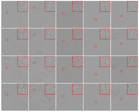
Figure 9.
Image Horizontal Visibility Graphs with for the ratio images. From top to bottom: Filtered with AE, FANS, Monet, and SCUNet.
4. Discussion
4.1. Visual Inspection
The despeckled images presented in Figure 1 show similar performance of several speckle reduction algorithms when applied to the SAR images chosen for this study. The top row of the figure corresponds to the SLC SAR image, which, as expected, exhibits a pronounced presence of multiplicative speckle noise.
Beneath the original image, the results of four despeckling approaches, namely, the AE, FANS, Monet, and SCUnet are displayed for comparison. Each method demonstrates distinct behavior in terms of speckle suppression, edge preservation, and structural fidelity. The AE method showed a strong ability to preserve image structure, edges, and fine details, indicating its capacity to retain textural and geometric features. However, it exhibited a limited ability to effectively suppress the noise, leading to residual speckle patterns in homogeneous areas. In contrast, the FANS filter achieved a substantial reduction in speckle intensity, yielding visually smoother regions, but at the cost of excessive smoothing that resulted in the loss of critical surface details and degradation of spatial information.
The Monet algorithm, although capable of modifying the intensity distribution, performed poorly in both speckle suppression and information preservation, producing results that appeared oversmoothed and lacking in relevant textural content. Finally, the SCUNet model, based on a convolutional neural network architecture, displayed spatially variable performance: it was effective in suppressing speckle over homogeneous regions such as water bodies, yet it failed to adequately remove noise in urban areas, where strong backscatter and complex geometrical structures are predominant.
4.2. Ratio Images
The ratio images presented in Figure 2 provide a visual assessment of the residual structural content that remains after the application of the different despeckling algorithms. Ideally, in a well-despeckled image, the corresponding ratio image should approximate a realization of iid random variables, exhibiting no discernible spatial patterns or correlated structures. However, the inspection of the results reveals that all filters retain a certain degree of residual structure, indicating that the despeckling process was not entirely effective in eliminating spatial dependencies introduced by the speckle or in perfectly preserving the statistical homogeneity of the scene.
Among the evaluated filters, Monet produced ratio images that most closely resemble uncorrelated random noise, suggesting that it is more effective in suppressing structured artifacts while maintaining a consistent radiometric response. The resulting textures in these cases exhibit minimal edge definition or directional patterns, implying a closer approximation to the expected stochastic behavior of a homogeneous noise field. On the other hand, the AE, FANS, and SCUNet algorithms display ratio images with noticeable structural remnants and edge-like formations, particularly along areas of high contrast or geometric complexity. This behavior suggests that these filters, while capable of preserving fine details and image boundaries, may also fail to keep structural information from the original image.
These observations indicate a trade-off between speckle suppression and structure preservation, which is intrinsic to most despeckling algorithms. Monet tends to favor statistical homogeneity at the expense of minor textural detail, while AE-, FANS-, and SCUNet-based approaches prioritize feature preservation, occasionally leading to the persistence of artificial structures in the ratio domain. Such behavior underscores the importance of combining visual inspection with quantitative analyses—such as texture metrics and divergence measures—to rigorously evaluate the degree of residual structure and the overall performance of each despeckling technique.
The Haralick features presented in Figure 4 and Figure 5 reveal that several of these texture descriptors exhibit significant inter-feature correlations, even when the pure-noise gamma image is included in the analysis. For example, while contrast and variance show low mutual correlation, both display high correlation with other Haralick measures. This observation suggests that the full set of Haralick features is redundant and that a reduced subset can adequately represent the textural information.
The selected, less correlated features are illustrated in Figure 6, where the features derived from the pure gamma image exhibit considerably higher values compared to those obtained from the AE, FANS, and Monet filters, which display similar behavior. In contrast, the SCUNet model produces markedly lower feature values, indicating a distinctive behavior that enables differentiation and facilitates a more detailed analysis of the despeckling performance.
A correlation analysis based on a pairplot of the two Haralick texture descriptors computed from images processed using different despeckling filters (AE, FANS, Monet, and SCUNet) and compared against a gamma distribution representing speckle noise is presented in Figure 7. The diagonal panels display the marginal kernel density estimations of each descriptor for the tested filters, while the off-diagonal plots illustrate their joint relationships, enabling visualization of inter-feature correlations.
The marginal distributions reveal that the AE, FANS, and Monet filters exhibit highly overlapping peaks for both descriptors, indicating similar texture profiles after despeckling. In contrast, the SCUNet filter shows distributions shifted toward significantly lower values, evidencing stronger smoothing and a consequent loss of texture information. The gamma distribution appears clearly separated, reflecting the distinct statistical behavior of raw speckle noise characterized by higher variability.
The scatter plots confirm a positive correlation between Contrast and Variance across all methods, where higher local contrast corresponds to greater variance. AE, FANS, and Monet produce compact clusters with moderate slopes, suggesting balanced noise reduction while maintaining structural texture. SCUNet forms a compact cluster in the low–low region, confirming an aggressive filtering approach. The gamma samples remain isolated, indicative of their non-filtered noise statistics.
From a discriminative perspective, SCUNet and gamma occupy distinct regions in the space, allowing clear differentiation from the other filters. Conversely, AE, FANS, and Monet overlap considerably, making them less distinguishable using only these two descriptors. This observation highlights the trade-off between smoothing strength and texture preservation: SCUNet favors maximum denoising at the expense of fine details, while AE, FANS, and Monet achieve a more balanced compromise.
Finally, the gamma reference underscores the statistical deviation introduced by despeckling, serving as a baseline for quantifying how effectively each filter suppresses the speckle signature. Overall, the results demonstrate that SCUNet exhibits the strongest smoothing effect, with notably low Contrast and Variance values. AE, FANS, and Monet maintain intermediate descriptor values, balancing speckle reduction and texture integrity. Gamma represents the statistical behavior of pure speckle noise and serves as a reference for evaluating filter performance.
The results of the -estimator presented in Table 1 exhibit a strong correlation with the metric, with a computed Pearson correlation coefficient of . This finding indicates that the estimator effectively captures the relationship between the values and the divergence obtained from the ratio images.
A comparative evaluation of the textural performance of different despeckling algorithms through the divergence-based metrics , , and (Table 2) are integrated into the proposed index , as defined in Equation (18). The results indicate that the Gamma model exhibits the highest divergence values (, ), acting as the ideal statistical reference representing pure speckle noise. In contrast, the AE, FANS, and Monet filters show intermediate values of and (ranging from to ) and low values (<0.1), which denotes a balanced trade-off between structural preservation and textural smoothing. Among all filters, FANS achieves the highest average texture-divergence score (), followed by Monet () and AE (), suggesting that its output is statistically closer to the gamma reference model while maintaining an adequate degree of textural homogeneity and detail preservation. Conversely, SCUNet presents extremely low and values (approximately, ) with an average , indicating a significant underestimation of textural variability and a tendency toward over-smoothing. Although this behavior reflects effective speckle suppression, it also implies a loss of fine structural information in the despeckled imagery.
Overall, these results demonstrate that filters such as FANS and Monet achieve a more balanced trade-off between noise suppression and structure preservation, whereas SCUNet exhibits excessive smoothing and loss of detail. The proposed normalized metric effectively discriminates these behaviors, confirming its suitability for comparative despeckling assessment.
The proposed metric is an effective quantitative measure for assessing the despeckling performance based on the statistical divergence of textural patterns with respect to a reference distribution. Its consistent behavior across multiple filters demonstrates its robustness as an integrated indicator of textural fidelity and statistical coherence in SAR despeckling applications.
4.3. Visibility Graphs
As seen in the first row of Figure 9, corresponding to the AE filter, the visibility graphs display relatively homogeneous and structure-free textures. The local patterns appear weak and spatially uncorrelated.
The FANS filter (Figure 9, second row) exhibits a similar behavior. The resulting graphs maintain a noise-like texture with minimal residual organization, confirming the filter’s ability to remove speckle while preserving the randomness expected in the ratio domain. Slight textural differences among samples may indicate minor variations in local adaptation but do not reveal significant structural remnants.
For the Monet filter (Figure 9, third row), the graphs show slightly more visible patterns and localized structures, particularly in the central regions of some samples. These residual textures suggest that, although Monet achieves a good level of despeckling, it preserves more spatial correlations than AE or FANS, leading to a less uniform noise representation.
In contrast, the SCUNet filter (Figure 9, fourth row) clearly departs from the ideal random texture. The visibility graphs exhibit structured patterns and spatial organization, indicating that this filter introduces or preserves deterministic components in the ratio images. This behavior suggests an over-smoothing effect combined with structural distortions, consistent with its low quantitative scores in , , and the composite metric.
5. Conclusions and Future Work
The proposed normalized metric () effectively integrates contrast (), variance (), and Jensen–Shannon Divergence () into a unified quantitative indicator, enabling a consistent and interpretable comparison of despeckling filters. The metric successfully discriminates filters that achieve a good balance between speckle suppression and structural preservation.
Quantitative evaluation results demonstrate that the FANS and Monet filters provide the best overall performance, with values of and , respectively. These filters yield ratio images that closely approximate the statistical properties of the reference gamma distribution, indicating effective despeckling with minimal loss of image information. Therefore constitutes a robust and unified indicator of textural divergence, effectively integrating contrast, variability, and informational similarity. It provides an objective and interpretable criterion for assessing the trade-off between speckle suppression and texture preservation, thereby improving the quantitative evaluation of despeckling filters in SAR image analysis.
The qualitative assessment using Image Horizontal Visibility Graphs (IHVGs) corroborates the numerical results. The graphs corresponding to AE and FANS exhibit noise-like, unstructured textures characteristic of properly despeckled images, whereas Monet and especially SCUNet show residual organized patterns that indicate remaining structural content.
Overall, the combined analysis confirms that the integration of statistical descriptors and graph-based texture analysis provides a comprehensive evaluation framework for despeckling performance. This dual approach allows distinguishing between filters that merely reduce variance and those that truly restore the statistical randomness expected in the ratio images.
Future research will focus on extending the proposed evaluation framework by incorporating additional statistical and perceptual metrics, as well as deep-learning-based texture descriptors, to further enhance the discrimination capability between despeckling methods. Moreover, the integration of spatial–temporal analysis and adaptive weighting strategies in the formulation could improve its generalization across different sensors, noise levels, and imaging conditions.
Author Contributions
R.D.V.-S.: Conceptualization, Methodology, Writing—Original Draft; W.S.P.: Methodology, Writing—Original Draft; L.G.: Conceptualization, Methodology, Formal Analysis, Writing—Review & Editing; A.C.F.: Conceptualization, Methodology, Formal Analysis, Writing—Review & Editing. All authors have read and agreed to the published version of the manuscript.
Funding
This research received no external funding.
Institutional Review Board Statement
Not applicable.
Informed Consent Statement
Not applicable.
Data Availability Statement
The original data presented in the study are openly available in [47].
Acknowledgments
Special thanks to the platforms Google Earth Engine (GEE), ASF Data Search Vertex of the University of Alaska, and the European Space Agency (ESA) for the open access availability Sentinel-1 SAR images used in this study.
Conflicts of Interest
The authors declare no conflict of interest.
Abbreviations
The following abbreviations are used in this manuscript:
| SAR | Synthetic Aperture Radar |
| CNN | Convolutional Neural Networks |
| ENL | Equivalent Number of Looks |
| MSE | Mean Squared Error |
| SSIM | Structural Similarity Index |
| PSNR | Peak Signal-to-Noise Ratio |
| PFOM | Pratt’s Figure of Merit |
| HVG | Horizontal Visibility Graphs |
| NVG | Natural Visibility Graphs |
| GLCM | Gray-Level Co-occurrence Matrix |
| SLC | Single Look Complex |
| GRD | Ground Range Detected |
| VV | Vertical Vertical |
| VH | Vertical Horizontal |
| AE | Auto-Encoder |
| FANS | Fast Adaptive Nonlocal SAR |
| Monet | Multi-Objective Network |
| SCUNet | Semantic Conditional U-Net |
References
- Wei, S.; Zeng, X.; Qu, Q.; Wang, M.; Su, H.; Shi, J. HRSID: A high-resolution SAR images dataset for ship detection and instance segmentation. IEEE Access 2020, 8, 120234–120254. [Google Scholar] [CrossRef]
- Argenti, F.; Lapini, A.; Bianchi, T.; Alparone, L. A Tutorial on Speckle Reduction in Synthetic Aperture Radar Images. IEEE Geosci. Remote Sens. Mag. 2013, 1, 6–35. [Google Scholar] [CrossRef]
- Lee, J.S. Digital image enhancement and noise filtering by use of local statistics. IEEE Trans. Pattern Anal. Mach. Intell. 1980, PAMI-2, 165–168. [Google Scholar] [CrossRef] [PubMed]
- Parrilli, S.; Poderico, M.; Angelino, C.V.; Verdoliva, L. A Nonlocal SAR Image Denoising Algorithm Based on LLMMSE Wavelet Shrinkage. IEEE Trans. Geosci. Remote Sens. 2012, 50, 606–616. [Google Scholar] [CrossRef]
- Zhang, Q.; Sun, R. SAR Image Despeckling Based on Convolutional Denoising Autoencoder. arXiv 2020, arXiv:2011.14627. [Google Scholar] [CrossRef]
- Xu, Q.; Xiang, Y.; Di, Z.; Fan, Y.; Feng, Q.; Wu, Q.; Shi, J. Synthetic Aperture Radar Image Compression Based on a Variational Autoencoder. IEEE Geosci. Remote Sens. Lett. 2022, 19, 4015905. [Google Scholar] [CrossRef]
- Vásquez-Salazar, R.D.; Cardona-Mesa, A.A.; Gómez, L.; Travieso-González, C.M. A New Methodology for Assessing SAR Despeckling Filters. IEEE Geosci. Remote Sens. Lett. 2024, 21, 4003005. [Google Scholar] [CrossRef]
- Wang, W.; Kang, Y.; Liu, G.; Wang, X. SCU-Net: Semantic Segmentation Network for Learning Channel Information on Remote Sensing Images. Comput. Intell. Neurosci. 2022, 2022, 8469415. [Google Scholar] [CrossRef]
- Amieva, J.F.; Ayala, C.; Galar, M. A deep learning approach to jointly super-resolve and despeckle Sentinel-1 imagery. Acta Astronaut. 2025, 238, 1396–1407. [Google Scholar] [CrossRef]
- Vitale, S.; Ferraioli, G.; Pascazio, V.; Deniz, L.G. Enhanced Deep Learning SAR Despeckling Networks based on SAR Assessing metrics. IEEE Geosci. Remote Sens. Lett. 2025, 22, 4009305. [Google Scholar] [CrossRef]
- Vitale, S.; Ferraioli, G.; Pascazio, V. Different Training Solution for Amplitude SAR Despeckling. In Proceedings of the IGARSS 2024—2024 IEEE International Geoscience and Remote Sensing Symposium, Athens, Greece, 7–12 July 2024; pp. 2176–2179. [Google Scholar]
- Kevala, V.D.; Nedungatt, S.; Lal, D.S.; Suresh, S.; Dell’Acqua, F. TransSARNet: A Deep Learning Framework for Despeckling of SAR Images. Eng. Res. Express 2025, 7, 0352b7. [Google Scholar] [CrossRef]
- Li, J.; Shi, S.; Lin, L.; Yuan, Q.; Shen, H.; Zhang, L. A multi-task learning framework for dual-polarization SAR imagery despeckling in temporal change detection scenarios. ISPRS J. Photogramm. Remote Sens. 2025, 221, 155–178. [Google Scholar] [CrossRef]
- Taher, A.; Al-Wadai, L.; Al-Malki, R. Residual U-Net for SAR Image Despeckling–a Lightweight and Effective Deep Learning Approach. In Proceedings of the 2025 IEEE Space, Aerospace and Defence Conference (SPACE), Big Sky, MT, USA, 1–8 March 2025; IEEE: Piscataway, NJ, USA, 2025; pp. 1–3. [Google Scholar]
- Bo, F.; Jin, Y.; Ma, X.; Cen, Y.; Hu, S.; Li, Y. SemDNet: Semantic-Guided Despeckling Network for SAR Images. Expert Syst. Appl. 2025, 296, 129200. [Google Scholar] [CrossRef]
- Sun, Z.; Zhang, Y.; Bao, M.; Yang, C.; Fan, P.; Zhang, W. SAR image despeckling based on differential attention and multi scale deep perception. IEEE Geosci. Remote Sens. Lett. 2025, 22, 4011005. [Google Scholar] [CrossRef]
- Wang, L.; Zhao, L.; Zhou, Z. A SAR image despeckling method combining Swin Transformer and DN-FPN. In Proceedings of the 2025 5th International Conference on Electronics, Circuits and Information Engineering (ECIE), Guangzhou, China, 23–25 May 2025; IEEE: Piscataway, NJ, USA, 2025; pp. 310–313. [Google Scholar]
- Guo, Z.; Hu, W.; Zheng, S.; Zhang, B.; Zhou, M.; Peng, J.; Yao, Z.; Feng, M. Efficient Conditional Diffusion Model for SAR Despeckling. Remote Sens. 2025, 17, 2970. [Google Scholar] [CrossRef]
- Cardona-Mesa, A.A.; Vásquez-Salazar, R.D.; Travieso-González, C.M.; Gómez, L. Comparative Analysis of Despeckling Filters Based on Generative Artificial Intelligence Trained with Actual Synthetic Aperture Radar Imagery. Remote Sens. 2025, 17, 828. [Google Scholar] [CrossRef]
- Frery, A.C.; Ospina, R.; Déniz, L.G. Finding structures in ratio images. In Proceedings of the 2015 IEEE International Geoscience and Remote Sensing Symposium (IGARSS), Milan, Italy, 26–31 July 2015; pp. 489–492. [Google Scholar]
- Déniz, L.G.; Buemi, M.E.; Jacobo-Berlles, J.; Mejail, M. A New Image Quality Index for Objectively Evaluating Despeckling Filtering in SAR Images. IEEE J. Sel. Top. Appl. Earth Obs. Remote Sens. 2016, 9, 1297–1307. [Google Scholar]
- Gómez, L.; Ospina, R.; Frery, A.C. Statistical Properties of an Unassisted Image Quality Index for SAR Imagery. Remote Sens. 2019, 11, 385. [Google Scholar] [CrossRef]
- Gómez, L.; Cardona-Mesa, A.A.; Vásquez-Salazar, R.D.; Travieso-González, C.M. Analysis of Despeckling Filters Using Ratio Images and Divergence Measurement. Remote Sens. 2024, 16, 2893. [Google Scholar] [CrossRef]
- Yue, D.X.; Xu, F.; Frery, A.C.; Jin, Y.Q. SAR Image Statistical Modeling Part I: Single-Pixel Statistical Models. IEEE Geosci. Remote Sens. Mag. 2021, 9, 82–114. [Google Scholar] [CrossRef]
- Frery, A.; Wu, J.; Gomez, L. SAR Image Analysis—A Computational Statistics Approach: With R Code, Data, and Applications; Wiley-IEEE Press: Hoboken, NJ, USA, 2022; ISBN 978-1-119-79546-9. [Google Scholar]
- Vitale, S.; Cozzolino, D.; Scarpa, G.; Verdoliva, L.; Poggi, G. Guided Patchwise Nonlocal SAR Despeckling. IEEE Trans. Geosci. Remote Sens. 2019, 57, 6484–6498. [Google Scholar] [CrossRef]
- Gomez, L.; Ospina, R.; Frery, A.C. Unassisted Quantitative Evaluation of Despeckling Filters. Remote Sens. 2017, 9, 389. [Google Scholar] [CrossRef]
- Lacasa, L.; Luque, B.; Ballesteros, F.J.; Luque, J.; Nuño, J.C. From time series to complex networks: The visibility graph. Proc. Natl. Acad. Sci. USA 2008, 105, 4972–4975. [Google Scholar] [CrossRef] [PubMed]
- Luque, B.; Lacasa, L.; Ballesteros, F.; Luque, J. Horizontal visibility graphs: Exact results for random time series. Phys. Rev. E—Stat. Nonlinear Soft Matter Phys. 2009, 80, 046103. [Google Scholar] [CrossRef]
- Iacovacci, J.; Lacasa, L. Visibility Graphs for Image Processing. IEEE Trans. Pattern Anal. Mach. Intell. 2018, 42, 974–987. [Google Scholar] [CrossRef]
- Haralick, R.M.; Shanmugam, K.S.; Dinstein, I. Textural Features for Image Classification. IEEE Trans. Syst. Man Cybern. 1973, 3, 610–621. [Google Scholar] [CrossRef]
- Jeevitha, V.; Aroquiaraj, I.L. Haralick Feature-Based Texture Analysis from GLCM and SRDM for Breast Cancer Detection in Mammogram Images. In Proceedings of the 2025 International Conference on Sensors and Related Networks (SENNET) Special Focus on Digital Healthcare(64220), Vellore, India, 24–27 July 2025; pp. 1–6. [Google Scholar] [CrossRef]
- Yadav, A.; Ansari, M.; Tripathi, P.; Mehrotra, R.; Jain, M. Braintumor and feature detection from MRI and CT scan using artificial intelligence. In Artificial Intelligence in Biomedical and Modern Healthcare Informatics; Elsevier: Amsterdam, The Netherlands, 2025; pp. 245–255. [Google Scholar]
- Le, D.B.T.; Narayanan, R.; Sadinski, M.; Nacev, A.; Yan, Y.; Venkataraman, S.S. Haralick Texture Analysis for Differentiating Suspicious Prostate Lesions from Normal Tissue in Low-Field MRI. Bioengineering 2025, 12, 47. [Google Scholar] [CrossRef]
- Raju, P.P.C.; Baskar, R. Comparison of GLCM and haralick features for analyzing textural variation in cotton leaf to identify spot disease. In Proceedings of the AIP Conference Proceedings; AIP Publishing LLC: Melville, NY, USA, 2025; Volume 3300, p. 020154. [Google Scholar]
- Nazyrova, D.; Aitkozha, Z.; Kerimkhulle, S.; Omarova, G. Combined approach based on Haralick and Gabor features to classify buildings partially hidden by vegetation. Sci. J. Astana IT Univ. 2025, 22, 88. [Google Scholar] [CrossRef]
- Arevalo, J.F.R.; Monge, H.F.A.; Vasquez, N.C.; Chipana, R.K.M. Analysis of the mathematical methods Haralick, Gabor and Wavelet applied to the recognition of soil textures. TPM- Psychom. Methodol. Appl. Psychol. 2025, 32, 2158–2167. [Google Scholar]
- Hasan, K.; Harb, H.; Elrefaei, L.A.; Abdel-Kader, H.M. Multi-channel Features Combined with Gray Features for Remote Sensing Image Classification. Mansoura Eng. J. 2025, 49, 17. [Google Scholar] [CrossRef]
- Martínez-Movilla, A.; Rodríguez-Somoza, J.L.; Arias-Sánchez, P.; Martínez-Sánchez, J. Comprehensive study of machine learning classification methods applied to UAV-based management of intertidal ecosystems. Remote Sens. Appl. Soc. Environ. 2025, 39, 101634. [Google Scholar] [CrossRef]
- Gajalakshmi, K.; Saravanan, S. Automatic identification of brittle, elongated and equiaxed ductile fracture modes in weld joints through machine learning. Sigma J. Eng. Nat. Sci./Mühendislik Fen Bilim. Derg. 2025, 43, 441–451. [Google Scholar] [CrossRef]
- Chandu, B.; Surendran, R.; Selvanarayanan, R. To Instant of Coffee Beans using K-nearest Algorithm Over Clustering for Quality and Sorting Process. In Proceedings of the 2024 International Conference on IT Innovation and Knowledge Discovery (ITIKD), Manama, Bahrain, 13–15 April 2025; IEEE: Piscataway, NJ, USA, 2025; pp. 1–7. [Google Scholar]
- Armin, E.; Ebrahimian, S.; Sanjari, M.; Saidi, P.; Pourreza, H.R. Defect detection in 3D printing: A review of image processing and machine vision techniques. Int. J. Adv. Manuf. Technol. 2025, 140, 2103–2128. [Google Scholar] [CrossRef]
- Nanda, M.A.; Saukat, M.; Yusuf, A.; Wigati, L.P.; Tanaka, F.; Tanaka, F. Identification of tomatoes with bruise using laser-light backscattering imaging technique. Sci. Hortic. 2025, 350, 114301. [Google Scholar] [CrossRef]
- Lin, J. Divergence measures based on the Shannon entropy. IEEE Trans. Inf. Theory 1991, 37, 145–151. [Google Scholar] [CrossRef]
- Menéndez, M.; Pardo, J.; Pardo, L.; Pardo, M. The Jensen-Shannon divergence. J. Frankl. Inst. 1997, 334, 307–318. [Google Scholar] [CrossRef]
- Vitale, S.; Ferraioli, G.; Pascazio, V. Multi-Objective CNN-Based Algorithm for SAR Despeckling. IEEE Trans. Geosci. Remote Sens. 2020, 59, 9336–9349. [Google Scholar] [CrossRef]
- Vásquez-Salazar, R.D.; Puche, W.S.; Frery, A.C.; Gómez, L. TDM. 2025. Available online: https://github.com/rubenchov/TDM (accessed on 15 October 2025).
Disclaimer/Publisher’s Note: The statements, opinions and data contained in all publications are solely those of the individual author(s) and contributor(s) and not of MDPI and/or the editor(s). MDPI and/or the editor(s) disclaim responsibility for any injury to people or property resulting from any ideas, methods, instructions or products referred to in the content. |
© 2025 by the authors. Licensee MDPI, Basel, Switzerland. This article is an open access article distributed under the terms and conditions of the Creative Commons Attribution (CC BY) license (https://creativecommons.org/licenses/by/4.0/).